On using of the proximal bundle method for nonsmooth optimization

(1)

Vysoká škola báˇnská – Technická univerzita Ostrava Fakulta elektrotechniky a informatiky

Katedra aplikované matematiky

Využití proximal bundle metody pro nehladkou

optimalizaci

On using of the proximal bundle method for

nonsmooth optimization

(2)

v g

- Technická univerzita ostrava Fakulta elektrotechniky a informatiky Katedra aplikované matematiky

Zadání

diplomové práce

student:

Bc.

Nikola Plí vová

Studijní

program:

N2647 Informační a komunikační technologie

Studijní

obor:

1103T031 Výpočetní matematika

Té ma:

Vyu ití

proximal

bundle metody pro nehladkou

optimalizaci

On using of the

proximal

bundle method for nonsmooth

optimization

Zásady pro vypracování :

Úloha minimalizace nediferencovatelné (nehladké ) funkce se objevuje při ře ení některých ú loh z mechaniky, např. kontakí ní ú lohy se tření m, ěi ú loh tvarové optimalizace. Tento problé m je mo né vyře it buď pří mo pomocí algoritmu vhodné ho pro minimalizaci nediferencovatelných funkcí , nebo nepří mo spojitě diferencovatelnou aproximací funkce a následně pomocí algoritmu vhodné ho pro minimalizaci spojitě diferencovatelných funkcí . V té to práci se věnujeme první mo nosti. Pro minimalizaci nediferencovatelných funkcí bylo vyvinuto vuplynulých desetiletí ch mnoho algoritmů. Mezi nejví ce pou í vané patří subgradientní metody a zejmé na bundle metody. Bundle metody mají řadu variant. Cí lem práce je jedna z nich _-proximal bundle metoda. Práce se zaměřuje na pochopení té to metody a její následnou efektivní implementaci.

V

závěru práce se budeme věnovat testování algoritmu na vhodných ú lohách.

Práce bude mí t _§ltočásti: Uloha nehladké optimalizace clarkeův kalkul

Algoritmy pro minimalizaci nediferencovatelných funkcí proximal _{bundle metoda}

Implementace proximal bundle metody Testování algoritmu na vhodných ú lohách

Seznam doporučené odborné literatury:

M.M.Miikelá, P.Neittaanmáki: Nonsmooth optimization. Singapore, World Scientií ic, 1992.

J. Zowe: Nondifferentiable optimization: A motivation and a short introduction into the subgradient and the bundle concept. In: NATO SAI Series, 15, Computational Mathematical Programming, Schittkowski, K., (ed.), Springer-Verlag, New York, 1985, pp. 323-356.

F.H. Clarke: Optimization and Nonsmooth Analysis. New York, John Wiley, 1983. Dále dle pokynů vedoucí ho diplomové práce.

(3)

Formální nále itosti a rozsah diplomové práce stanoví pokyny pro vypracování zveřejněné na webových stránkách fakulty.

Vedoucí diplomové práce: Ing. Petr Beremlijski, Ph.D.

Datum

zadání :

0L09.20l4

Datumodevzdání :

07.05.2015

EU,-,l*/.-

C-,1

doc. RNDr. Jiří Bouchala, Ph.D. vedoucí lratedry

RNDr. Václav Sná el, CSc. děkanfafulty

(4)

”Pure mathematics is, in its way, the poetry of logical ideas.”

(5)

I

Prohla uji, e jsem tuto diplomovou práci vypracovala samostatně. Uvedla jsem v echny literární prameny a publikace, ze kí erýchjsem čerpala.

4r'

"o"{

V Orlové dne 4.května 2015

(6)

I would like to thank Ing. Petr Beremlijski, PhD. for his patience, very valuable advice and constant support, which help to create this diploma thesis.

(7)

Abstract:

In practical applications we often have to solve the problem where the cost function is not differ-entiable. Thus we cannot directly use methods like Gradient Descent or Newton’s methods. The aim of this thesis is to introduce method and implement an algorithm for nonsmooth optimization, namely the Proximal Bundle one. After briefly familiarization with a general optimization problem, we devote several chapters to nonsmooth analysis and optimization theory. The penultimate chapter consists of relatively detailed description of Proximal Bundle method algorithm and in the last part we summarize some numerical results obtained by our implementation in MATLAB.

Keywords:

Optimization, nonsmooth function, nonsmooth optimization, Subgradient method, Proximal Bundle method.

Abstrakt:

V praktických aplikacích se ˇcasto setkáváme s problémy, kdy cenová funkce není diferencovatelná. V tomto pˇrípadˇe nelze pˇrímo využít metod, jako jsou napˇríklad gradientní ˇci Newtonova metoda. Cílem této práce je pˇredstavit metodu a implementovat algoritmus pro nehladkou optimalizaci, konkrétnˇe metodu Proximal Bundle. Po krátkém seznámení se s obecnou optimalizaˇcní úlohou, vˇenujeme nˇekolik kapitol teorii nehladké analýzy a optimalizace. Pˇredposlední kapitola obsahuje relativnˇe detailní popis algoritmu Proximal Bundle metody a v poslední kapitole jsou shrnuty výsledky numerických experiment˚u naší implementace v MATLABU.

Klíˇcová slova:

Optimalizace, nehladká funkce, nehladké optimalizace, Subgradientní metoda, Proximal Bundle metoda.

(8)

5.1.2 Subgradient aggregation . . . 31 5.1.3 Nonconvexity . . . 33 5.2 Line search . . . 34 5.3 Weight update . . . 37 5.4 Algorithm . . . 39 5.4.1 Convergence analysis . . . 41 5.4.2 Algorithm implementation . . . 41 6 Numerical experiments 43 6.1 Tested functions . . . 43 6.2 Numerical results . . . 47 7 Conclusion 53 References 54 A CD description 55 B Algorithms 57

(10)

List of Tables

2.1 Algorithm of gradient descent. . . 5

2.2 Algorithm of Newton’s method. . . 7

4.1 Basic Algorithm. . . 21

4.2 Results forx0= [−3; 4]andε= 10−3. . . 24

4.3 Results forx0= [−3; 4]andε= 10−5. . . 25

4.4 Results forx0= [7;−12]andε= 10−3. . . 25

4.5 Results forx0= [7;−12]andε= 10−5. . . 25

5.1 Algorithm Line search. . . 36

5.2 Algorithm Weight Update. . . 38

5.3 Algorithm Proximal Bundle. . . 39

6.1 Results of Proximal Bundle methods - precisionε= 10−3. . . 48

6.2 Results of Proximal Bundle methods - precisionε= 10−6. . . 49

(11)

List of Figures

2.1 Small ball over the obstacle. . . 3

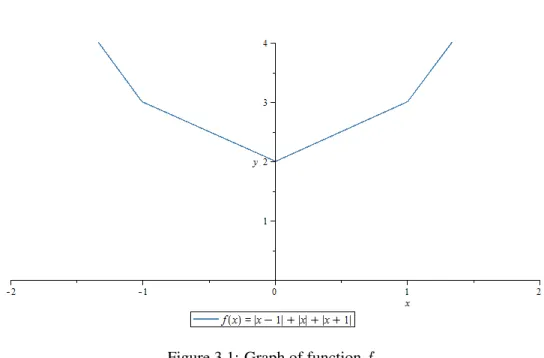
3.1 Graph of functionf. . . 11

3.2 Graph of the general gradient off atx= 0. . . 12

3.3 Graph of the general gradient off. . . 12

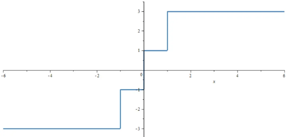
3.4 Graph of the Goldsteinε-subdifferential off atx∈Rfor_ε_{= 0}_.₁. . . 13

3.5 Graph of the Goldsteinε-subdifferential off atx∈(−1.5,1.5)forε= 1.5. . . . 14

3.6 Graph of the Goldsteinε-subdifferential off. . . 15

3.7 Convergence to the nonoptimal point. . . 18

3.8 Lacking of an implementable stopping rule. . . 19

4.1 Graph of functionf =|x1|+|x2|. . . 23

4.2 Graph of contours and solution. . . 26

6.1 Graph of functionf(x) = 100(x2−x12)2+ (1−x1)2. . . 44

6.2 Graph of functionf(x) =|x1|+|x2|. . . 44

6.3 Graph of functionf(x) = max{x2₁+ (x2−1)2+x2−1,−x21−(x2−1)2+x2+ 1}. 45 6.4 F1- Convergence of the sequence{xi}∞i=1 ⊂Rnand convergence to the optimal valuef(x). . . 49

6.5 F2- Convergence of the sequence{xi}∞ i=1 ⊂Rnand convergence to the optimal valuef(x). . . 50

6.6 F3- Convergence of the sequence{xi}∞i=1 ⊂Rnand convergence to the optimal valuef(x). . . 50

6.7 F4- Convergence to the optimal valuef(x). . . 51

(12)

Listings

B.1 Subgradient method . . . 57 B.2 Line search . . . 58 B.3 Weight update . . . 59 B.4 Proximal Bundle . . . 60 IX

(13)

List of symbols

Rn _n-dimensional Euclidean space

A n×nmatrix

A−1 _{inverse matrix}

AT transposed matrix b, v n-dimensional vectors

C1_(Ω) _{space of function with continuous first derivative}

C2(Ω) space of function with continuous second derivative

∇f(x) gradient of functionf f′₍_x₎ _{the first derivation of}_f

f′′(x) the second derivation off Hf(x) Hessian matrix

conv(Ω) convex hull of setΩ

∂f(x) general gradient of functionf gf subgradient of functionf ∂f(x)G

ε the Goldsteinε-subdifferential of functionf f′(x;v) directional derivative off atxin the directionv

f∘(x;v) general directional derivative off atxin the directionv

t↓0 t→0+

�(Rn₎ set of all subsets inRn

B(x;ε) open ball with radiusεand central pointx NΩ(x) normal cone of the convex setΩatx

arg minf(x) a point wheref has its minimum

‖x‖ Euclidean norm

Jk

f index set

˜

Jk

f subset on an index setJfk

lim sup

x→x0

f(x) an upper limit of functionf

(14)

1 Introduction

The classical optimization methods are used for differentiable functions. Unfortunately, we some-times have situation where the cost function is not necessarily differentiable. This obstacle is solved variously: e.g. approximation by smooth function, which also brings us other difficulties in the form of approximation errors. That is one of the reasons why the theory of nonsmooth optimization was initiated.

The aim of this thesis is to introduce nonsmooth optimization method - namely Proximal Bundle method and implement an algorithm. The text is divided into five parts, which are put in this order. The first part consists of optimization theory principles. It is only an introduction to the optimization theory. We also describe here the differences between several types of the optimization programming. Some solution methods can be found there too.

Before we concentrate on the nonsmooth optimization, we have to devote to the nonsmooth analysis and optimization theory. The material of the second part consists of many definitions and theorems, which helps us to understand the requirements to the cost function property and optimality condi-tions. A failure of classical methods is described there, because this is another reason why we need to invent different solving methods.

In the third chapter, we consider a short introduction to the nonsmooth optimization and the solution methods - like Subgradient method and Bundle method. Since the Bundle method (Proximal Bundle method) is analysed in the next part, the Subgradient method occupies a larger part of this chapter. We can read there something about choosing the step size and about stopping rule. The influence of the step size choice is shown in the example.

The last two chapters are devoted to the Proximal Bundle method. After a survey of the optimiza-tion methods and analysis, we construct an algorithm for nonsmooth problems. We can find there a detailed algorithm description and a summary of our numerical results. We have tested some traditional examples.

Another important part of the thesis is a CD containing the algorithms of Subgradient and Proximal Bundle methods.

(15)

2 An optimization problem

The aim of this chapter is to introduce the basic principles of the optimization. Also we describe differences among the various types of the optimization and we write some information about the solution methods.

We draw inspiration from [1] and [2].

2.1 Introduction

An optimization problem in mathematics is a problem of finding the best element from all elements which are feasible. We use a cost function to decide which one is the best. In the general way, the cost function is a representationf : � → R, where_�is a set of elements from a suitable

vector space. In many cases, we are trying to find extremes of some cost function in a feasible setΩ⊆ �. As the minimum of functionf is the same as the maximum of function−f, we can consider the general optimization problem as findingx∈Ωsuch that

f(x)≤f(x), x∈Ω. (2.1) We can also write this problem in this way

︂

minimize f(x)

subject to x∈Ω. (2.2)

Both of this writing describes the same optimization problem. In our text we will use the second one. Solution of this problem is called aglobal solution.

(16)

2.2 Classification of optimization methods 3

For better imagination, we can mention as an example finding a steady state of small ball on a spring pendent over a obstacle. This problem can be represented as a minimization of potential energy function. Feasible set describes parts where small ball doesn’t get through the obstacle. So we have to solve problem ︂ minimize f(x) subject to x∈Ω, (2.3) wheref(x) =x2₁+x2₂+m·x2,Ω = ︀ x∈R_: _x2 1+x2−4≥0,−x1−x2+ 5≥0 ︀ andmis the ball weight.

Figure 2.1: Small ball over the obstacle.

In the example below, we can see that the setΩis restricted, soΩ⊂ � andΩ ̸=�. This type of problem is calledconstrained optimization. In the case whenΩ = �, we are talking about

unconstrained optimization.

2.2 Classification of optimization methods

There are several types of optimization methods. It insists on a cost functionf and also on function h, which describes equality or inequality. Both of these functions are defined at� ⊂Rn, hence we

are talking about smooth optimization. 2.2.1 Linear programming

General problem of linear programming is specified by linear functionb∈Rnand by restriction

B∈Rm×nand_c_∈Rm.

It can be written this way:

Findx∈Ωsuch thatbT_x_≤_bT_x_{for all}_x_∈_Ω_,

(17)

2.3 Solution methods 4

2.2.2 Quadratic programming

General problem of quadratic programming is different only in quadratic cost function, which is described in symmetrical matrixA∈Rn×nand in_b_∈Rn. This problem can be written like this:

Findx∈Ωsuch that1₂xTAx−bTx≤ 1₂xTAx−bTxfor allx∈Ω

whereΩis described by linear equation mentioned in linear programming. 2.2.3 Nonlinear programming

When the cost function is neither linear nor quadratic but it is smooth with smooth first derivation at least, we are talking about nonlinear programming. IfΩ∈Rn, so the area is not restricted, we

have special type of nonlinear programming where we can use special algorithms. When we don’t know anything about cost function and about binds, we have a very difficult problem which can be solved only by using algorithms, that have specified characteristic.

2.2.4 Nonsmooth programming

Nonsmooth programming is used when the cost function and the bind function are smooth except a small subset of domain. This partial smoothness can be employed for creating effective algorithms. This type of problem is commonly more difficult then nonlinear ones. First difficulties is in complicated description of minimal condition because the function needn’t be differentiate in solution.

2.3 Solution methods

There are many methods which can be used for searching minima of function. Every method has its own request, so it helps us to decide which one we will use to solve some problem. Usually we want the functionf to be continuous(f ∈C(Ω))also to have continuous its first(f ∈ C1(Ω))

(the best the second(f ∈C2(Ω))) derivation. In the case when the functionf ∈C1(Ω), we can use gradient of the function and in the case whenf ∈C2_(Ω)_{, we use Hessian and Newton methods.}

(18)

2.3.1 Gradient descent method

This method uses the negative direction of the gradient at the given point to find a local minimum of a function. It’s a first-order optimization algorithm because it employs only first derivative of a function, so this function has to beC1(Ω). A basic algorithm is mentioned below for better understanding.

Algorithm 2.1: Algorithm of gradient descent.

Step 0: Inputx0, ε >0.

Step 1: Setk= 1andxk=x0.

Step 2: while‖∇f(x)‖< ε dk=−_‖∇∇f_f(₍x_x)₎_‖ tk =argmin t>0 f(xk+t·dk) xk+1=xk+tkdk k=k+ 1 end Step 3: Outputxk.

(19)

2.3.2 Newton’s method Forx∈R

This method is employed for finding better approximation to the roots of function. Using Newton’s method, we are trying to find whenf(x) = 0. Geometrically,(xk+1,0)is the intersection with

the x axis of the tangent to the graph of functionf at(xk, f(xk)). We can find the next value ofx

using this equation

xk+1=xk− f(xk) f′₍_x

k)

. (2.4)

Similar equation is used to find minimum of functionf xk+1 =xk− f′₍_x k) f′′₍_x k) , (2.5)

because the derivative of function in extreme is zero. As you can see, the function f has to be inC2_(Ω)_{, so the condition are quite strict.}

Also we can derive this method from the second order Taylor expansionfT(x)of a functionf

aroundxn, wherexnis a sequence (constructed with Newton’s method from initial point) that converges toward exact resultx. Thisxis a stationary point off, so we know, thatf′(x) = 0. Let △x=x−xn. Then we can write Taylor expansion

fT(xn+△x) =fT(xn) =f(xn) +f′(xn)△x+1 2f

′′₍_xn₎_△_x2_. _(2.6)

We attain its extreme when derivative with respect to△x= 0, so△xsolves this equation

f′(xn) +f′′(xn)△x= 0 =⇒ −f

′₍_xn₎

f′′₍_x

n)

=△x. (2.7)

Now we know that functionf is well approximated by its second order Taylor expansion. When the initial pointx0is well chosen, then the sequence(xn)

△x=x−xn=−f ′₍_xn₎ f′′₍_xn₎, (2.8) xn+1=xn− f′(xn) f′′₍_xn₎, forn= 0,1, . . . (2.9)

(20)

Algorithm 2.2: Algorithm of Newton’s method.

Step 0: Inputx0, ε >0.

Step 1: Setk= 1andxk=x0− f

′₍_x 0) f′′₍_x₀₎. Step 2: while‖xk−xk−1‖< ε xk+1=xk− f ′₍_x k) f′′₍_x k) k=k+ 1 end Step 3: Outputxk. Forx∈Rn

We can generalized Newton’s method to more dimension if we replace the first derivative with gradient of function and the second derivative with the Hessian matrixHf(x).

So

(21)

3 Nonsmooth analysis

In this chapter, we get acquainted with the theoretical basis of nonsmooth analysis and with the attributes, which every tested function should have. Concurrently, we show why we cannot use algorithms introduced in Chapter 2 for a nonsmooth optimization.

We draw inspiration from [1], [3], [4] and [6], so more information can be found there.

3.1 Convex set

Definition 3.1.1. We denote by⟨x, y⟩the close line segment joiningxandyby

⟨x, y⟩={z∈Rn_|_z₌_λx_{+ (1}₋_λ₎_yfor₀_≤_λ_≤₁_}_. (3.1)

A setΩ⊂Rnis calledconvexif_⟨x, y⟩ ⊂Ωfor allxandybelonging toΩ.

3.2 Convex hull

Definition 3.2.1. LetΩ⊂Rn. Then_conv_(Ω)denotesconvex hullof set_Ω. (The set of all convex

combinations of points inΩ.) conv(Ω) = ︃ _n ︁ i=1 λixi|n∈N_{, λ}_∈Rn_{, x}₁_,_{· · ·}_{, xn}_∈_Ω_{, λi} _≥₀_,_∀_i, n ︁ i=1 λi = 1 ︃ (3.2)

3.3 Convex function

Definition 3.3.1. A functionf :Rn_→Ris said to beconvexinRnif

f(λx+ (1−λ)y)≤λf(x) + (1−λ)f(y),∀x, y∈Rn_,_∀_λ_{∈ ⟨}₀_,₁_⟩_. (3.3)

(22)

3.4 Locally Lipschitz continuity 9

3.4 Locally Lipschitz continuity

Definition 3.4.1. A functionf :Rn_→Rislocally Lipschitz continuous with constant Lat_x_∈Rn

if there exists some constantε >0such that

|f(y)−f(z)| ≤L‖y−z‖,∀y, z ∈B(x;ε). (3.4) Definition 3.4.2. A functionf : Ω ⊂Rn_→ Ris said to belocally Lipschitz continuouson_Ωif

there exists some constantL=L(Ω)>0such that

|f(x)−f(y)| ≤L‖x−y‖,∀x, y∈Ω. (3.5) Definition 3.4.3. A functionf :Rn _→Ris said to belocally Lipschitz continuousinRnif for

everyΩ⊂Rn, where_Ωis a compact set, exists some constant_L₌_L_(Ω)_>₀such that

|f(x)−f(y)| ≤L‖x−y‖,∀x, y∈Ω. (3.6)

3.5 Generalized directional derivative

Definition 3.5.1. Let f : Rn _→ R be locally Lipschitz continuous at a point _x _∈ Rn_. The

generalized directional derivativeoff atxin the direction ofv∈Rnis defined by

f∘(x;v) = lim sup

y→x t↓0

f(y+tv)−f(y)

t . (3.7)

3.6 General gradient and subgradient

Theorem 3.6.1. (Rademacher). LetΩ ⊂Rnbe an open set and_f _{: Ω}_→ Rbe Lipschitz with

constantKonΩ. Thenf is differentiable almost everywhere onΩ.

Proof. Please see [4] or [6]. ₂

Definition 3.6.2. Let f : Rn _→ R be locally Lipschitz continuous (inRn). Then the general

gradientoff atx∈Rnis the set

∂f(x) =conv ︂ g∈Rn ⃒ ⃒ ⃒ ⃒ g= lim∇f(xi), xi →x ∇f(xi)exists,∇f(xi)converges ︂ . (3.8)

(23)

3.7ε-subdifferential 10

3.7 ε

-subdifferential

ε-subdifferential is a modification of the classic subdifferential used in nonsmooth optimization. Now we give the definition and its basic properties.

Definition 3.7.1. Letf :Rn _→ Rbe locally Lipschitz continuous (inRn). Thenthe Goldstein

ε-subdifferentialis the set

∂f(x)G_ε =conv ︂ g∈Rn ⃒ ⃒ ⃒ ⃒ g= lim∇f(yi), yi→y ∇f(yi)exists,∇f(yi)converges, y∈B(x;ε) ︂ . (3.9) Each elementg∈∂f(x)G

ε is calledε-subgradientof the functionf atx.

Theorem 3.7.2. Letf :Rn_→Rbe locally Lipschitz continuous with constant_Lat_x. Then

(i) ∂f(x)G 0 =∂f(x). (ii) Ifε1 < ε2, then∂f(x)Gε1 ⊂∂f(x) G ε2. (iii) ∂f(x)G

ε is a nonempty, convex, compact set such that‖g‖< Lfor allg∈∂f(x)Gε.

(iv) The mapping∂f(·)Gε :Rn→ �(Rn)is upper semi-continuous.1

Proof. The proof can be found in [4]. 2

Corollary 3.7.3. Letf :Rn_→Rbe locally Lipschitz continuous at_x. If_ε_≥₀_,then

∂f(y)⊂∂f(x)G_ε for ally∈B(x;ε). (3.10) Note. Written theory is for general function, but we can also find definitions and theorems especially for convex functions. Please see [4] or [6]. We don’t need to mention it in this thesis, because we will solve problems with general cost functions.

1_{A function}

f:Rn_→Ris said to beupper semi-continuousat_xif for every sequence_{_x_i_}converging to_xwe have

lim sup

i→∞

(24)

3.7.1 Example - general gradient and the Goldsteinε-subdifferential

Lets explain written theory on a simple example.

Find the general gradient and the Goldsteinε-subdifferential of functionf at a given pointx.

f(x) =|x−1|+|x|+|x+ 1|

Figure 3.1: Graph of functionf. Another expression of the functionf is

f(x) = ⎧ ⎪ ⎪ ⎨ ⎪ ⎪ ⎩ −3x x∈(−∞;−1) −x+ 2 x∈ ⟨−1; 0) x+ 2 x∈ ⟨0; 1) 3x x∈ ⟨1;∞).

(25)

The general gradient

Write and plot the general gradient off atx = 0. We will use definition 3.6.2. We have to use one-sided limit becausex= 0is a point where the functionfis not smooth.

For

xi→0+ : g= 1

xi→0− : g=−1 ︂

∂f(x) =conv{−1,1}

Figure 3.2: Graph of the general gradient off atx= 0. The general gradient off for allx∈Ris

(26)

The Goldsteinε-subdifferential

Write the Goldsteinε-subdifferential off atx= 0for differentεusing theorem 3.7.1. Set ∙ ε1 = 0.1 Theny∈(−0.1,0.1) y∈(−0.1,0) : yi →y⇒ g=−1 y∈(0,0.1) : yi →y⇒ g= 1 y= 0 : yi →0⇒ g∈ ⟨−1,1⟩ ⎫ ⎬ ⎭ ∂f(x)Gε1 =conv{−1,1}

We can find the Goldsteinε-subdifferential off at everyx∈(−0.1,0.1). Here we can see a graph for allx∈(−0.1,0.1).

(27)

3.7ε-subdifferential 14 ∙ ε2 = 1.5 Theny∈(−1.5,1.5) y∈(−1.5,−1) : yi →y⇒ g=−3 y∈(−1,0) : yi →y⇒ g=−1 y∈(0,1) : yi →y⇒ g= 1 y∈(1,1.5) : yi →y⇒ g= 3 y=−1 : yi → −1⇒ g∈ ⟨−3,−1⟩ y= 0 : yi →0⇒ g∈ ⟨−1,1⟩ y= 1 : yi →1⇒ g∈ ⟨1,3⟩ ⎫ ⎪ ⎪ ⎪ ⎪ ⎪ ⎪ ⎪ ⎪ ⎬ ⎪ ⎪ ⎪ ⎪ ⎪ ⎪ ⎪ ⎪ ⎭ ∂f(x)Gε2 =conv{−3,−1,1,3}

As in the example above, also here we can find the Goldsteinε-subdifferential off at every x∈(−1.5,1.5). Here we can see a graph for allx.

Figure 3.5: Graph of the Goldsteinε-subdifferential offatx∈(−1.5,1.5)forε= 1.5.

Here we can see an example of theorem 3.7.2 (ii)

Ifε1< ε2, then∂f(x)Gε1 ⊂∂f(x)

G ε2

(28)

Now we write the Goldsteinε-subdifferential atx= 0.05. ∙ ε1 = 0.1 Theny∈(−0.05,0.15) y∈(−0.05,0) : yi →y⇒ g=−1 y∈(0,0.15) : yi →y⇒ g= 1 y= 0 : yi →0⇒ g∈ ⟨−1,1⟩ ⎫ ⎬ ⎭ ∂f(x)G_ε1 =conv{−1,1}

The Goldsteinε-subdifferential off for allx∈Rand_ε_{= 0}_.₁is

(29)

3.8 Optimality conditions 16

3.8 Optimality conditions

We should specify the basic necessary conditions at minimizerxfor unconstrained problem. Also we have to note, that for convex functions these conditions are sufficient forxwhich is the minimum

of function. All the theorems and proofs were inspired or taken from [4].

Theorem 3.8.1. Iff :Rn_→Ris locally Lipschitz at_xand attains its local minimum at_x, then

(i) 0∈∂f(x)and

(ii) f∘(x;v)≥0for allx∈Rn.

Proof. Suppose first that f attains a local minimum at x.Then there exists ε > 0 such that

f(x+tv)−f(x)≥0for all0< t < εandv∈Rn. Now we have

f∘(x;v) = lim sup y→x t↓0 f(y+tv)−f(y) t ≥lim supt↓0 f(x+tv)−f(x) t ≥0 hands f∘(x;v)≥0 = 0Tv for all v ∈Rn_,

which means by the definition of subdifferential that0∈∂f(x). 2

Theorem 3.8.2. Iff :Rn_→Ris convex, then the following condition are equivalent:

(i) fattains its global minimum atx, (ii) 0∈∂f(x),

(iii) f′₍_x_;_v₎_≥₀_{for all}_x_∈_Rn_.1

Proof. The assertion (ii) follows from (i) by Theorem 3.8.1(i). Supppose next, that (ii) holds. By Theorem 2.1.5. in [4] we have for allv∈Rn

f′(x;v) = max{ξTv|ξ∈∂f(x)} ≥0Tv= 0.

To complete the proof it suffices now to show that (iii) implies (i). To see this, considerx′∈Rn.

We have

f′(x;x′−x) = max{ξT(x′−x)|ξ ∈∂f(x)} and so there existsξx′ ∈∂f(x)such that

0≤f′(x;x′−x) =ξ_xT′(x′−x).

Then it follows that

f(x′)≥2f(x) +ξ_xT′(x′−x)≥f(x),

which means thatf attains its global minimum atx. 2

1_{If the function}

fis convex, thenf∘(x;v) =f′(x;v).

(30)

3.8 Optimality conditions 17

Next theorems are listed without proofs. To see them please look into [4], where all the omitted proofs can be found.

Theorem 3.8.3. Iff :Rn_→Ris locally Lipschitz at_xand attains its local minimum at_x, then

0∈∂_εGf(x). (3.11)

Theorem 3.8.4. Iff :Rn_→Ris convex, then the following condition are equivalent:

(i) 0∈∂G ε f(x),

(ii) xminimizesf withinε, i.e.f(x)≤f(y) +εfor ally∈Rn.

We need this following theorem to write optimality conditions for constrained problems. Theorem 3.8.5. The normal coneof the convex setΩatx∈Ωis the set

NΩ(x) ={z∈Rn|(x′−x)Tz≤0for allx′ ∈Ω} (3.12)

Now we can write conditions for constrained problems.

Theorem 3.8.6. Iff is locally Lipschitz atxand attains its local minimum over the setΩ⊂Rn

atx, then

0∈∂f(x) +NΩ(x). (3.13)

Theorem 3.8.7. Iff :Rn _→Ris convex and the setΩis convex, then the following condition are equivalent:

(i) 0∈∂f(x) +NΩ(x),

(31)

3.9 Failure of classical methods 18

3.9 Failure of classical methods

In a classical smooth method, we usually use linear or quadratic model which leads to steepest descent or to Newton’s method. Obviously, these two methods are not useful if a function is not smooth. There are two types of problem when classical methods fail.

3.9.1 Convergence to the nonoptimal point

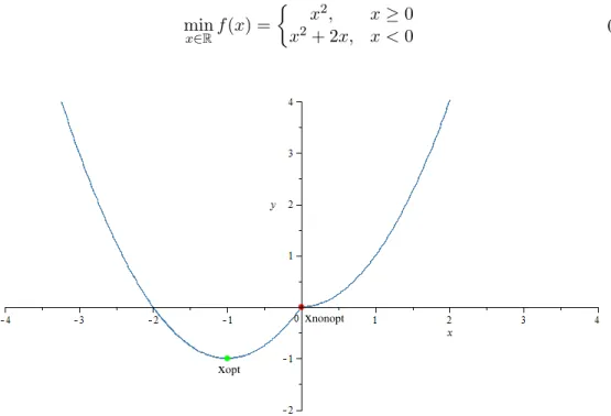
Both of mentioned methods don’t work at a kink of function. It can caused that we will be trapped at a nonoptimal kink and methods give us bad results. It is evident in this example

min

x∈Rf(x) =

︂

x2_, _x_≥₀

x2+ 2x, x <0 (3.14)

Figure 3.7: Convergence to the nonoptimal point.

Set the given pointx0= 2. After few iterations, methods will give us resultx= 0, but as we can

(32)

3.9 Failure of classical methods 19

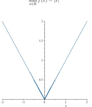
3.9.2 Lacking of an implementable stopping rule

Letf ∈C1_(Ω)_{. The the gradient will be small in norm when we approach some optimal point.}

|∇f(xk)| ≤ε (ε >0small)

This can help us to implement some stopping rule. But let see at this example

min

x∈Rf(x) =|x| (3.15)

Figure 3.8: Lacking of an implementable stopping rule.

At eachxk̸= 0, whenxkis close to the optimal kinkx= 0, we have|∇f(xk)|= 1. The steepest descent method will not stop close to thexbecause the gradient is not close to zero.

(33)

4 Nonsmooth optimization

In this part, we consider the nonsmooth optimization. After a very short description, we write there about solution methods like Subgradient method and Bundle methods and we give en example of using Subgradient method.

This chapter is inspired by [5] and [4].

4.1 Introduction

Let the cost functionf :Rn_→Rto be only locally Lipschitz function on the feasible set_Ω_⊂Rn.

Consider also the optimization problem

︂

minimize f(x)

subject to x∈Ω, (4.1)

which is nonlinear and constrained. Whenf is continuously differentiable then the problem (4.1) is

called smooth and ifΩ =Rnthen it is unconstrained.

Optimization methods are iterative. This means, that it begins at a given initial pointx1 ∈Rnand

then it constructs a sequence{xi}∞

i=1⊂Rnwhich intends to converge to the solution we required.

A general basic iterative algorithm is mentioned below. (Taken from [4])

(34)

Algorithm 4.1: Basic Algorithm.

Step 0: (Initialization) Find a feasible starting pointx1 ∈Ωand setk= 1.

Step 1: (Direction finding) Find a feasible descent directiondk∈Rn:

f(xk+tdk)< f(xk)andxk+tdk∈Ωfor somet >0.

Step 2: (Stopping criterion) Ifxkis "close enough" to the required solution then STOP. Step 3: (Line search) Find a step sizetk>0such that

tk≈argmin

t>0{f(xk+tdk)}andxk+tdk∈Ω

Step 4: (Updating) Setxk+1 =xk+tkdk, k=k+ 1and go on to Step 1.

4.2 Solution methods

As you can read in the part 2.3, we can find solution by using first order or second order meth-ods when the cost function is differentiable. In this thesis, we are especially interested in non-differentiable functions, so we can’t use mentioned methods and we have to find another way to solve this problem. Which methods can be employed, we describe in this part.

4.2.1 Subgradient method

Suppose for now the cost functionf is smooth. In a standard first order or second order method, we make a feasible descent direction along the negative gradient(−∇f(x))or along the negative gradient scaled by Hessian matrix︀

(−∇2_f₍_x₎₎−1_{· ∇}_f₍_x₎︀

. For nonsmooth, locally Lipschitz cost function the gradient shouldn’t exists in every point of the function, but we have at least one subgradient. Now it is obvious, how we can substitute the gradient. The feasible descent direction

dkin the basic algorithm 4.1 can be find in this waydk= gk

‖gk‖ (gkis subgradient atxk) and then

the updating part will be

xk+1 =xk+tk

gk

‖gk‖

, k=k+ 1.

Unfortunately, this simple idea poses two critical problems: how we can choose the step sizetkand

is there any implementable stopping rule? Choosing the step sizetk

Let begin with the first task: How to choose the step sizetk? We have to consider two cases.

In the first one, we know function value of some optimal pointxand in the second one the function value in optimal point is not known.

(35)

Function value in optimal point is known

In this case, the step sizetkcan be chosen this way:

∙ Also we can compute this special step size which guarantees a monotonous decrease for allk tk= λ(f(xk)−f(x))

‖gk‖ where0< λ <2.

We don’t knowf(x)a priori. ∙ Constant step size:tk =const

∙ A priori chosen step size which has to fulfil conditions: i) tk→0+;

ii) ︀∞ k=0

tk =∞.

∙ tk=M pkwhereM >0and0< p <1

This is only the sum of the ways how to settk, to read more about this issue see [5].

Stopping rule

Unfortunately, the cost function is not smooth, so the gradient shouldn’t become smaller as soon as we are closer to the optimal point. As we illustrated it in the part 3.9.2, it is very difficult to implement any stopping rule. This is one of the negative attribute.

(36)

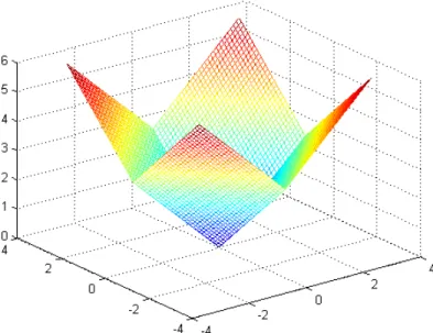
4.2.2 Example - Subgradient method Minimizef(x), x∈R2where

f(x) =|x1|+|x2|. (4.2)

Figure 4.1: Graph of functionf =|x1|+|x2|.

Solution

To find an optimal point, we use MATLAB m-files. First we need to implement some routine which helps us to compute subgradients at every point of a domain even at point of discontinuity. We have to split the domain into 4 parts:

I. x1, x2≥0

II. x1 <0andx2 ≥0

III. x1 ≥0andx2 <0

(37)

and in every part we need to count up partial derivatives I. ∂f ∂x1 = 1 ∂f ∂x2 = 1 ︃ = [1; 1] II. ∂f ∂x1 =−1 ∂f ∂x2 = 1 ︃ = [−1; 1] III. ∂f ∂x1 = 1 ∂f ∂x2 =−1 ︃ = [1;−1] IV. ∂f ∂x1 =−1 ∂f ∂x2 =−1 ︃ = [−1;−1]

Due to 3.6.2 we can assemble general gradient off(x)

∂f(x) =conv{[1; 1],[−1; 1],[1;−1],[−1;−1]}. (4.3)

We implemented some routine which gives us value of subgradient corresponding to certain part. Now we can use mentioned m-files to find a minimum. We employed Subgradients method with step sizetk = 1_k (1st. type) andtk = λ(f(xk)−f(x))

‖gk‖ , whereλ = 1and xis the optimal point

(2nd. type).

Results can be seen in the following tables.

∙ Set starting pointx0= [−3; 4]and precisionε= 10−3

Type Minimum Number of iterations

(1st. type) [0;−0.7071·10−3] 1001

(2nd. type) [−0.1110·10−15;−0.1110·10−15] 4

(38)

∙ Set starting pointx0= [−3; 4]and precisionε= 10−5

(1st. type) [0;−0.7071·10−5_] ₁₀₀₀₀₁

(2nd. type) [−0.1110·10−15_;₋₀_.₁₁₁₀_·₁₀−15_] ₄

Table 4.3: Results forx0 = [−3; 4]andε= 10−5.

∙ Set starting pointx0= [7;−13]and precisionε= 10−3

(1st. type) [0.9992;−6.9992] 1002

(2nd. type) [−0.4441·10−15_;₋₀_.₄₄₄₁_·₁₀−15_] ₄

Table 4.4: Results forx0 = [7;−12]andε= 10−3.

∙ Set starting pointx0= [7;−13]and precisionε= 10−5

(1st. type) [0;−3.7439] 100001

(2nd. type) [−0.4441·10−15;−0.4441·10−15] 4

Table 4.5: Results forx0 = [7;−12]andε= 10−5.

Subgradient method (2nd. type) gave us results much faster then (1st. type), because this method uses better direction finding. In the next picture, we can see contours off(x), the starting point

(39)

Figure 4.2: Graph of contours and solution. 4.2.3 Bundle methods

Another methods employed to solve problems with the nonsmooth cost function are Bundle methods, which were published in 1975 for the first time. These methods are working under the next precondition:

∙ In everyx∈Rnwe know_f₍_x₎and at least one subgradient_g_∈_∂f₍_x₎.

The main difference between Subgradient methods and Bundle methods are in these features: ∙ In every iteration the subgradient is gathered into a bundle (that’s why these methods have

their name)

– If the chosen descent directiondkdoesn’t give us a sufficient effect, we stay in the same iteration pointxk+1 =xkbut the subgradient is added into a bundle. This is callednull

step.

– Otherwise we make aserious step- subgradient is also added into a bundle and we set

xk+1=xk+tkdk.

∙ Through knowledge of the subgradient we can implement a stopping rule.

This is a brief introduction. In the next chapter we will devote specifically to Proximal Bundle method more in details.

(40)

5 Proximal Bundle method

As we mentioned above, this chapter is devoted to the Proximal Bundle method. A detailed algorithm description can be found there. This algorithm is divided into several parts - Direction finding, Line search, Weight update and the main Proximal Bundle algorithm.

It this chapter, we draw inspiration from [4], [6] and [7]. Consider the following problem

minimize f(x)

subject to x∈Rn

︂

(P)

wherefis locally Lipschitz function. We suppose that we can evaluate at eachx∈Rnsubgradients

gf _∈_∂f₍_x₎_{and the function value}_f₍_x₎_{. Our task is to find the direction}_d_∈_Rn_{, which solves} minimize f(xk+d)−f(xk)

subject to d∈Rn_,

︂

(5.1) if the current iteration pointxk ∈ Rn is not optimal. We will employ theH function defined

aty∈Rnby

H(x;y) =f(x)−f(y),forallx∈Rn_,

so the general problem(P)can be modified hereby

minimize H(xk+d;xk) subject to d∈Rn_.

︂

(HP)

5.1 Direction finding

For a while, we suppose that the problem(P)is convex. The nonconvex case will be considered later.

5.1.1 Derivation of the direction finding problem

Suppose that we have the current iteration pointxk ∈ Rn, xk ̸= x1(starting point), auxiliary

pointyj ∈ Rnand subgradients _g_jf _∈ _∂f₍_yj₎ for_j _∈_J_fk _{⊂ {}₁_{, . . . , k}_}where the index set_J_fk

(41)

5.1 Direction finding 28

is nonempty.

Let define the linearization atxk∈Rnby

fj(x) =f(x;yj) =f(yj) + (gf_j)T(x−yj); j∈J_fk (5.2) Also we define the polyhedral approximation for allx∈Rnby

ˆ

fk(x) = max{fj(x)|j∈Jfk} (5.3)

wherefj(x)is represented in this way

f_j(x) =f_jk+ (g_jk)T(x−xk); j∈J_fk (5.4) denotedfk

j =fj(xk). Considering the polyhedral approximation, we have to redefine functionH

as follows

ˆ

Hk(x) = ˆfk(x)−f(xk) for allx∈Rn_. (5.5)

Theorem 5.1.1. The polyhedral approximation functionHˆk(x)is convex. If in addition the

prob-lem (P) is convex, then

ˆ

Hk(x)≤H(x;xk) for allx∈Rn. (5.6)

Proof. As maxima of affine functions the polyhedral approximationsfˆk₍_x₎_{are convex, thus}_H_ˆk

is also convex. If the problem is convex, then (due to the definition of subgradient) linearizations

fj are lower approximations of the problem functions. 2

Employing Proximal Bundle idea1_{with using the approximated function}_Hˆk_{, we obtain the next}

approximation to(HP) minimize Hˆ(xk+d) +uk 2 ‖d‖2 subject to d∈Rn_. ︂ (GCP)

We shall use following notation to balance the presentation

αk_f,j =f(xk)−f_jk forj ∈J_fk (5.7) substitutingf_jkwe obtain

αk_f,j =f(xk)−f(yj)−(gf_j)T(xk−yj) forj∈J_fk. (5.8)

The(GCP)problem can be rewritten, but we have to employ the definition (5.3) which means, that

ˆ

fk(xk+d)≥f(yj) + (gjf) T₍_x

k−yj). (5.9)

Furthermore, the function

ˆ

Hk(xk+d)≥fˆk(xk+d)−f(xk) for allxk+d∈Rn_. (5.10)

(42)

5.1 Direction finding 29 Then ˆ Hk(xk+d)≥fˆk(xk+d)−f(xk)≥ ≥f(yj) + (gf_j)T(xk+d−yj)−f(xk) = =f(yj) + (gf_j)T(xk−yj) + (gjf) T_d₋_f₍_x k) = =−αk_f,j+ (gf_j)Td. (5.11)

Denotingv= ˆHk₍_xk₊_d₎_{, we rewrite the}_(GCP)_{problem this way}

minimize v+uk 2 ‖d‖2 subject to −αk f,j+ (g f j)T(d)≤v for allj∈Jfk. ︃ (BP)

The(BP)problem in this form is called a primal (minimization) problem. In optimization theory we can also used a dual form of the problem. This duality means that the optimization problems can be viewed from a different perspective, where we supposed to find multipliers solving the dual problem. Let’s try to derive the dual form of(BP).

First, we should assemble Lagrange function of(BP).

L(v, d, λ) =v+uk 2 ‖d‖ 2₊ k ︁ j=1 λj(−αkf,j+ (g f j) T_d₋_v₎ _(5.12)

and also the Karush–Kuhn–Tucker conditions of(BP). 1. ∇v,dL(v, d, λ) = 0 2. λj(−αk_f,j + (g_jf)Td−v) = 0for allj ∈J_fk 3. λj ≥0 4. v≥ −αk f,j + (g f j)Td

Applying the first condition we obtain

∇v,dL(v, d, λ) = ⎡ ⎢ ⎢ ⎢ ⎣ 1− ︀k j=1 λj ukd+ k ︀ j=1 λjg_jf ⎤ ⎥ ⎥ ⎥ ⎦ = 0 (5.13) then follows 1− k ︁ j=1 λj = 0⇒ k ︁ j=1 λj = 1 (5.14) ukd+ k ︁ j=1 λjgf_j = 0⇒d= − k ︀ j=1 λjg_jf uk . (5.15)

(43)

From the second condition we have

k ︁ j=1 λj(−αk_f,j + (g_jf)Td−v) = 0 − k ︁ j=1 λjαk_f,j+ k ︁ j=1 λj(g_jf)Td= k ︁ j=1 λjv. (5.16)

Substitutedfrom (5.15) into (5.16) we obtain

− k ︁ j=1 λjαkf,j+ k ︁ j=1 λj(g_jf)T ⎛ ⎜ ⎜ ⎜ ⎝ −︀k j=1 λjgjf uk ⎞ ⎟ ⎟ ⎟ ⎠ =v k ︁ j=1 λj (5.17)

Using (5.14) we can expressv

− k ︁ j=1 λjαk_f,j − 1 uk ⃦ ⃦ ⃦ ⃦ ⃦ ⃦ k ︁ j=1 λjgf_j ⃦ ⃦ ⃦ ⃦ ⃦ ⃦ 2 =v. (5.18)

Now we have expression fordandv, so we can substitute them into Lagrangian and we obtain

min x maxλ L(v, d, λ) max λ − k ︁ j=1 λjαf,jk − 1 uk ⃦ ⃦ ⃦ ⃦ ⃦ ⃦ k ︁ j=1 λjgjf ⃦ ⃦ ⃦ ⃦ ⃦ ⃦ 2 +uk 2 ⃦ ⃦ ⃦ ⃦ ⃦ ⃦ ⃦ ⃦ ⃦ −︀k j=1 λjgjf uk ⃦ ⃦ ⃦ ⃦ ⃦ ⃦ ⃦ ⃦ ⃦ 2 max λ − k ︁ j=1 λjα_f,jk − 2 2uk ⃦ ⃦ ⃦ ⃦ ⃦ ⃦ k ︁ j=1 λjg_jf ⃦ ⃦ ⃦ ⃦ ⃦ ⃦ 2 + 1 2uk ⃦ ⃦ ⃦ ⃦ ⃦ ⃦ k ︁ j=1 λjg_jf ⃦ ⃦ ⃦ ⃦ ⃦ ⃦ 2 max λ − k ︁ j=1 λjα_f,jk − 1 2uk ⃦ ⃦ ⃦ ⃦ ⃦ ⃦ k ︁ j=1 λjg_jf ⃦ ⃦ ⃦ ⃦ ⃦ ⃦ 2 min λ 1 2uk ⃦ ⃦ ⃦ ⃦ ⃦ ⃦ k ︁ j=1 λjgf_j ⃦ ⃦ ⃦ ⃦ ⃦ ⃦ 2 + k ︁ j=1 λjαk_f,j (5.19)

So via dualization we can solve the next problem

minimize ₂1_u k ⃦ ⃦ ⃦ ⃦ ⃦ k ︀ j=1 λjgjf ⃦ ⃦ ⃦ ⃦ ⃦ 2 + ︀k j=1 λjαf,jk subject to ︀k j=1 λj = 1 λj ≥0for allj ∈Jk f ⎫ ⎪ ⎪ ⎪ ⎪ ⎪ ⎪ ⎬ ⎪ ⎪ ⎪ ⎪ ⎪ ⎪ ⎭ (DP)

(44)

5.1.2 Subgradient aggregation

There is still one task to solve. How can we choose the index setJk

f? This set is a nonempty subset

of{1, . . . , k}. We have to solve many problem with storage and computation in practice. To avoid big memory requirement, we will employ the subgradient aggregation strategy. So we would like to aggregate the constraints generated by past subgradient, which helps us to keep the number of constraints within certain limits.

Definition 5.1.2. Letλk

j forj∈Jfkbe Lagrange multipliers of the problem(BP)at iterationk. We

define the aggregate subgradients by

pk_f = ︁ j∈Jk f λk_jgf_j (5.20) ˜ f_pk = ︁ j∈Jk f λk_jf_jk (5.21) ˜ αk_f,p= ︁ j∈Jk f λk_jαk_f,j (5.22)

and the aggregate linearization by

˜

fp(x) = ˜f_pk+ (pk_f)T(x−xk) (5.23)

Lemma 5.1.3. The(BP)problem is equivalent to the reduced problem

minimize v+ uk 2 ‖d‖2 subject to −αk f,j + (g f j)T(d)≤v for allj∈J˜fk −α˜k f,p+ (pkf)T(d)≤v ⎫ ⎪ ⎬ ⎪ ⎭ (RP) where_J˜k f is any subset ofJfk.

Proof. Please see [4] ₂

Now we can solve the(RP)problem which seems to be appropriate for keeping the index set finite. However, it presents a problem as well. At the beginning of every iteration, the vectorpk

f is not

known. This problem can be eliminated recursively. Letx1 ∈Rnbe a feasible starting point, then

the algorithm seems like

y1=x1 p0f =g f

1 ∈∂f(y1) fp1 =f11 =f(y1) J ={1}.

At iterationkthe unknown vectorsf˜pk,p˜kf will be replaced by the previously generatedfpk, pkf−1

and also we define

αk_f,p=f(xk)−fpk (5.24)

which leads to the problem

minimize v+ uk

2 ‖d‖2

subject to −αk_f,j + (g_jf)T(d)≤v for allj∈J˜_fk

−αk f,p+ (p k−1 f )T(d)≤v ⎫ ⎪ ⎬ ⎪ ⎭ (ABP)

(45)

Also here we can try to derive the dual form of(ABP).

As before, we should assemble Lagrange function of(ABP)first

L(v, d, λ) =v+uk 2 ‖d‖ 2₊ k ︁ j=1 λj(−αk_f,j+ (g_jf)Td−v) +λp(−αk_f,p+ (pk_f−1)T(d)−v) (5.25) and also the Karush–Kuhn–Tucker conditions of(ABP)

1. ∇v,dL(v, d, λ) = 0 2. λj(−αk f,j + (g f j)Td−v) = 0for allj ∈Jfk 3. λp(−αk f,p+ (p k−1 f )T(d)−v) = 0 4. λj, λp≥0 5. v≥ −αk_f,j + (g_jf)Td 6. v≥ −αk_f,p+ (p_fk−1)T(d)

Applying the first condition we obtain

∇v,dL(v, d, λ) = ⎡ ⎢ ⎢ ⎢ ⎣ 1− k ︀ j=1 λj−λp ukd+ k ︀ j=1 λjgf_j +λppk_f−1 ⎤ ⎥ ⎥ ⎥ ⎦ = 0 (5.26) then follows 1− k ︁ j=1 λj−λp = 0⇒ k ︁ j=1 λj +λp = 1 (5.27) ukd+ k ︁ j=1 λjgf_j +λppk_f−1 = 0⇒d= −︀k j=1 λjg_jf −λppk_f−1 uk . (5.28)

Adding up the second and the third conditions we have

k ︁ j=1 λj(−αkf,j+ (g f j) T_d₋_v_{) +}_λ p(−αf,pk + (pkf−1) T₍_d₎₋_v_{) = 0} − k ︁ j=1 λjαkf,j + k ︁ j=1 λj(gfj) T_d₋_λ pαkf,p+λp(pkf−1) T_d₌ k ︁ j=1 λjv+λpv − k ︁ j=1 λjαkf,j −λpαkf,p+d ⎛ ⎝ k ︁ j=1 λj(gjf) T ₊_λ p(pkf−1) T ⎞ ⎠=v ⎛ ⎝ k ︁ j=1 λj+λp ⎞ ⎠. (5.29)

(46)

Substitutingdfrom (5.28) into (5.29) and using (5.27) we can expressv

− k ︁ j=1 λjαkf,j−λpαkf,p− 1 uk ⎛ ⎝ k ︁ j=1 λjg_jf+λppk_f−1 ⎞ ⎠ ⎛ ⎝ k ︁ j=1 λjg_jf +λppk_f−1 ⎞ ⎠=v − k ︁ j=1 λjαkf,j −λpαkf,p− 1 uk ⃦ ⃦ ⃦ ⃦ ⃦ ⃦ k ︁ j=1 λjgjf +λppkf−1 ⃦ ⃦ ⃦ ⃦ ⃦ ⃦ 2 =v (5.30)

Now we have expression fordandv, so we can substitute them into Lagrangian and we obtain

min x maxλ L(v, d, λ) max λ − k ︁ j=1 λjαk_f,j −λpαk_f,p− 1 uk ⃦ ⃦ ⃦ ⃦ ⃦ ⃦ k ︁ j=1 λjg_jf +λppk_f−1 ⃦ ⃦ ⃦ ⃦ ⃦ ⃦ 2 +uk 2 ⃦ ⃦ ⃦ ⃦ ⃦ ⃦ ⃦ ⃦ ⃦ −︀k j=1 λjgf_j −λppk_f−1 uk ⃦ ⃦ ⃦ ⃦ ⃦ ⃦ ⃦ ⃦ ⃦ 2 max λ − k ︁ j=1 λjαkf,j −λpαkf,p− 2 2uk ⃦ ⃦ ⃦ ⃦ ⃦ ⃦ k ︁ j=1 λjgfj +λppkf−1 ⃦ ⃦ ⃦ ⃦ ⃦ ⃦ 2 + 1 uk ⃦ ⃦ ⃦ ⃦ ⃦ ⃦ k ︁ j=1 λjgjf +λppkf−1 ⃦ ⃦ ⃦ ⃦ ⃦ ⃦ 2 max λ − k ︁ j=1 λjαk_f,j −λpαk_f,p− 1 2uk ⃦ ⃦ ⃦ ⃦ ⃦ ⃦ k ︁ j=1 λjgf_j +λppk_f−1 ⃦ ⃦ ⃦ ⃦ ⃦ ⃦ 2 min λ 1 2uk ⃦ ⃦ ⃦ ⃦ ⃦ ⃦ k ︁ j=1 λjg_jf +λppk_f−1 ⃦ ⃦ ⃦ ⃦ ⃦ ⃦ 2 + k ︁ j=1 λjαk_f,j +λpαk_f,p (5.31) So via dualization we can solve this problem

minimize ₂_u1 k ⃦ ⃦ ⃦ ⃦ ⃦ k ︀ j=1 λjg_jf +λppk_f−1 ⃦ ⃦ ⃦ ⃦ ⃦ 2 + k ︀ j=1 λjαk f,j+λpαkf,p subject to k ︀ j=1 λj+λp = 1 λj, λp ≥0. ⎫ ⎪ ⎪ ⎪ ⎪ ⎪ ⎪ ⎬ ⎪ ⎪ ⎪ ⎪ ⎪ ⎪ ⎭ (ADP) 5.1.3 Nonconvexity

For convex function the linearisation error increases as far as we are from a given point. We can’t take advantage of this attribute when we have nonconvex function. Due to this fact, we have to generalize the linearisation errors. We shall employ so-calledsubgradient locality measures1_,

which were described for the first time by Kiwiel.

(47)

5.2 Line search 34

Definition 5.1.4. We definedistance measureat each iterationkby

sk_j ⎧ ⎨ ⎩ ‖xj−yj‖+ k−1 ︀ i=j ‖xi+1−xi‖ forj= 1, . . . , k−1, ‖xk−yk‖ forj=k, (5.32) theaggregate distance measuresby

⎧ ⎨ ⎩ ˜ sf_k =︀ j∈ ˜ λk jskj + ˜λkpskf, sf_k₊₁ = ˜sf_k+‖xk+1−xk‖, (sf1 = 0) (5.33) and thesubgradient locality measuresby

⎧ ⎪ ⎨ ⎪ ⎩ β_f,jf = max{|αk f,j|, γf(skj)2} for allj∈J˜fk, β_f,pf = max{|αk f,p|, γf(skf)2}, ˜ β_f,pf = max{|α˜k f,p|, γf(˜skf)2}, (5.34)

whereγf ≥0is thedistance measure parameter(γf = 0)for convex functionf.

5.2 Line search

Suppose that we have found a solution(dk, vk)of the(ABP)problem at the k-th iteration with the subgradient locality measures. Also, we have to remember that this is solution for_Hˆk_{which only}

approximatesH, so the chosen directionxk+1 =xk+dkneedn’t to be the best one. therefore we

will try to find a feasible step sizetk∈(0,1]such that

tk≈arg min tk∈(0,1]

{f(xk+tdk)} andxk+tdk∈Rn. (5.35)

Unfortunately, the directiondkmay not be necessarily the descent one or the descending is not sufficient. That’s why we have to modify the general line search.

To detect discontinuities in the gradient off, we will describe a two-point line search. We assume

that ⎧ ⎪ ⎪ ⎨ ⎪ ⎪ ⎩ mL= (0,1₂) mR= (mL,1) t= (0,1] ζ = 1−1₂ ·₁₋1_m L (5.36)

(48)

5.2 Line search 35

Now we will search the largest numbertk

L∈[0,1]such that

a)f(xk+tkLdk)≤f(xk) +mLtkLvk

b)tk_L≥t (5.37)

If suchtk

Lexists we have

∙ a long serious step: xk+1 =xk+tkLdk yk+1 =xk+1,

if (5.37)(a) is held while0< tk

L< tthen we have

∙ a short serious step: xk+1=xk+tkLdk yk+1=xk+tkRdk

and iftk

L= 0we have

∙ a null serious step: xk+1=xk

yk+1 =xk+tkRdk

wheretk

R> tkLis such that

c) −β_f,kk+1₊₁+ (gf_k₊₁)T_dk_≥_mRvk _(5.38)

In long serious step, there is no reason to detect discontinuities in the gradient off and we set gf_k₊₁ ∈∂f(xk+1).

In short and null step, there is a discontinuity so the new subgradient will beg_kf₊₁ ∈∂f(yk+1)and

it will constrain a modification of the next direction finding problem.

At the next line of this thesis, we will show an algorithm of a line search method where conditions a) - c) are held.

(49)

5.2 Line search 36

Algorithm 5.1: Algorithm Line search.

Step 1: Settk L= 0andt=tU = 1. Step 2: If f(xk+tdk)≤f(xk) +mLtvk settk L=t, otherwise settU =t.

Step 3: Iftk_L≥tsettk_R=tk_Land STOP, otherwise calculategf ∈∂f(xk+tdk)and

β = max{|f(xk+tkLdk)−f(xk+tdk) + (t−tkL)(gf)Tdk|, γf(t−tkL)2‖dk‖2}.

Then if

−β+ (gf)Tdk≥mRvk,

settk

R=tand STOP.

Step 4: Iftk_L= 0, then set

t= max{ζ·tU, 1 2t2Uvk tUvk+f(xk)−f(xk+tUdk)} and iftk L>0, then sett= 12 ·(tkL+tU). Step 5: Go on toStep 2.

(50)

5.3 Weight update 37

5.3 Weight update

We cannot choose the weightuksuch that it is constant, because it brings several difficulties.

∙ Ifuk is very large, we can obtain |vk|and‖dk‖ too small. Due to this, all steps will be

serious and decline will be small.

∙ Ifukis very small, then|vk|and‖dk‖is too large and every serious step is followed by many

null steps.

So we need to keep it up as variable and change its value whet it is necessary.

In 1990 K. C. Kiwiel presented a safeguarded quadratic interpolation technique for updating

uk.

We will detect whetherukis not too large after we have a long serious step(tL= 1). As we can

see in the section 5.2, we haveyk+1 =xk+dkand

f(yk+1)≤f(xk) +mLvk (5.39)

and if

f(yk+1)≤f(xk) +mRvk (5.40)

we will decreaseuk. To decrease it we will use this quadratic interpolation

uintk = 2uk(1−[f(yk+1)−f(xk)]/vk). (5.41)

In the case where condition (5.40) is not held, we also decreaseukby updating

uk+1= max{uk/2, umin}. (5.42)

We will test if

β_f,kk+1₊₁>max︁‖pk‖+ ˜βpk,−10vk ︁

(5.43) is held after we have many successive null steps. When this condition is fulfilled, theukis increased

and updated by

uk+1= min

︀

uint_k₊₁,10uk︀

(5.44)

(51)

5.3 Weight update 38

Algorithm 5.2: Algorithm Weight Update.

Step 1: Setu=uk. Step 2: IftL∈(0,1)STOP. Step 3: Else iftL= 0. Set εk_v+1= min︁εk_v,‖pk‖+ ˜βpk ︁ . Ifik u <−3and β_f,kk+1₊₁>max︁ε_vk+1,−10vk︁, setu=uint k+1. Set uk+1= min{u,10uk}, iku+1= min ︁ iku−1,−1 ︁ . Ifuk+1 ̸=uksetiku+1=−1.STOP. Step 4: Else. Set εk_v+1= max︁εk_v,−2vk︁. Ifik u >0and f(yk+1)≤f(xk) +mRvk, setu=uint k+1, otherwise, ifik u >3setu=uk/2. Set

uk+1 = max{u, uk/10, umin},

ik_u+1= max︁ik_u+ 1,1︁.

(52)

5.4 Algorithm 39

5.4 Algorithm

Now we can present the Proximal Bundle method for nonconvex unconstrained optimization. Algorithm 5.3: Algorithm Proximal Bundle.

Step 0(Initialization): Select some starting pointx1 ∈ Rn, an accuracy toleranceεs > 0, the

maximum number of stored subgradientsMg≥2, an initial weightu1 >0, a weights lower

boundumin, line search parametersmL ∈ (0,1₂), mR ∈ (mL,1)and t ∈ (0,1].Set the

distance measure parameterγf >0(for convex functionγf = 0), iteration counterk = 1, count the line search parameterζ = 1− 1₂·₁₋1_m

L and initialize variables:

︃

y1 =x1, p0f =g f

1 ∈∂f(y1), fp1 =f11 =f(y1)

s1_f =s1₁ = 0, J1 ={1}.

Step 1(Direction finding): Find multipliersλk

p,λkj forj ∈Jfkby solving this dual problem ⎧ ⎪ ⎪ ⎪ ⎪ ⎪ ⎪ ⎨ ⎪ ⎪ ⎪ ⎪ ⎪ ⎪ ⎩ minimize ₂1_u k ⃦ ⃦ ⃦ ⃦ ⃦ k ︀ j=1 λjg_jf +λppk_f−1 ⃦ ⃦ ⃦ ⃦ ⃦ 2 + k ︀ j=1 λjαk f,j +λpαkf,p subject to k ︀ j=1 λj+λp= 1 λj, λp≥0. where βk f,j = max ︁ |f(xk)−fjk|, γf(skj)2 ︁ for all j ∈Jk f, βk f,p= max ︁ |f(xk)−fk p|, γf(skf)2 ︁ . Also set pk f = ︀ j∈Jk f λk jg f j +λkppkf−1, ˜ fk p = ︀ j∈Jk f λk jfjk+λkpfpk, ˜ sk f = ︀ j∈Jk f λk_jf_jk+λkpskf, ˜ βk f,p= max ︁ |f(xk)−f˜pk|, γf(˜skf)2 ︁ anddk=−_u1_kpk

(53)

5.4 Algorithm 40

Step 2(Stopping criterion): Set

wk= 1 2‖pk‖

2_{+ ˜}_βk f,p

Ifwk ≤εsthen STOP.

Step 3(Line search): Using line search algorithm mentioned in the section 5.2 find step size

tk

L∈[0,1]andtRk ∈[tkL,1]. Set

xk+1 =xk+tkLdk and yk+1=xk+tkRdk.

Step 4(Linearization update): Calculate the values

f_jk+1=fk j +tkL(g f j)Tdk, for j∈Jfk, sk_j+1 =sk_j +t_Lk‖dk‖, for j∈J_fk, fk+1 p = ˜fpk+tkL(p f f)Tdk, sk_f+1 = ˜sk f +tkL‖dk‖.

Evaluategf_k₊₁ ∈∂f(yk+1)and set

f_kk₊₁+1 =f(yk+1) + (tkL−tkR)(g f j)Tdk, sk_k+1₊₁ = (tk

R−tkL)‖dk‖.

Step 5(Weight updating): Selectuk+1by the algorithm in the section 5.3.

Step 6(Updating): SetJ_fk+1 =Jk

f ∪ {k+ 1}, but ifJ k+1

f > Mg, then J_fk+1 =J_fk+1∖ {minj|j∈J_fk+1}. Increase k by 1 a go onStep 1.

(54)

5.4 Algorithm 41

5.4.1 Convergence analysis

∙ Convex functionf

Theorem 5.4.1. Put

X* ={x*∈Rn_|_f₍_x*₎_≤_f₍_x_{) for all}_x_∈Rn_}_.

IfX* ̸=∅the{xk}converges to somex∈X*ask→ ∞. IfX* ₌_∅_the_{_f₍_x

k)}converges to someinf{f(x)|x∈Rn} ∈[−∞;∞).

∙ Nonconvex functionf

Theorem 5.4.2. Letf be weakly semi-smooth1_{and locally Lipschitz on}_Rn_{. If}_f_{is bounded}

below and{xk}is bounded, then there exists a cluster pointx˜of the sequence{xk}such

that0∈∂f(˜x).

Proof. Both of the proofs can be found in [6]. 5.4.2 Algorithm implementation

We should show how we implement theStep 1in the Proximal Bundle method algorithm. This algorithm was implemented in MATLAB, which has many internal functions. In the direction finding part, we want to usequadprogso we have to modify the dual problem(ADP)into form

min

x

1 2x

T_Hx₊_fT_x,

that thisquadprogfunction requires.

Compilation of matrix H and vectors x,f. Lets rewrite 1 2 ⃦ ⃦ ⃦ ⃦ ⃦ k ︀ j=1 λjgj +λppf ⃦ ⃦ ⃦ ⃦ ⃦ 2

into matrix notation.

1 2 ⃦ ⃦ ⃦ ⃦ ⃦ ⃦ k ︁ j=1 λjgj+λppf ⃦ ⃦ ⃦ ⃦ ⃦ ⃦ 2 = 1 2 ⃦ ⃦ ⃦ ⃦ ⃦ ⃦ k+1 ︁ j=1 ˜ λj˜gj ⃦ ⃦ ⃦ ⃦ ⃦ ⃦ 2 = = 1 2 ⎛ ⎝ k+1 ︁ j=1 ˜ λjg˜j ⎞ ⎠ T⎛ ⎝ k+1 ︁ j=1 ˜ λjg˜j ⎞ ⎠= = 1 2λ˜ T_GT_G_˜_λ₌ 1 2˜λ T₍_GT_G_)˜_λ₌ = 1 2λ˜ T_H_λ_˜ (5.45)

(55)

5.4 Algorithm 42 So G=︀ pf, g1, g2, . . . , gk ︀ , (5.46) H= 1 ukG T_G, _(5.47) ˜ λ=︀ λp, λ1, λ2, . . . , λk ︀T (5.48) and ˜ β=︀ βf,p, βf,1, βf,2, . . . , βf,k ︀T . (5.49)

MatrixGand vectors_λ˜_,_β˜_{have on its first position an aggregate element. Due to the limit of stored}

subgradientsMg, we have to solve how to rewrite the next elements ofG,˜_λ_and_β˜_{. In every iteration,}

we test if size of matrix and vectors is higher thenMg. If it does, we delete the second column

(or element) and add a new one at the end. If it doesn’t, we don’t delete anything. Now we can rewrite the(ADP)problem into quadratic problem

minimize 1₂˜λT_H_λ_˜₋_λT_β_˜ subject to Aλ˜=B LB≤˜λ≤U B ⎫ ⎬ ⎭ (QP) whereA= [1,1, . . . ,1],B= [1],LB= [0,0, . . . ,0]T _and_{U B} _{= [}_∞_,_∞_{, . . . ,}_∞_]T_.

(56)

6 Numerical experiments

After a detailed algorithm description in the previous chapter, we shall report some numerical experiments to show reliability of our code. The Proximal Bundle method was implemented in MATLAB 2012a. A summary of all the tests can be found in this part.

6.1 Tested functions

We have tested some traditional examples. Here we can see a summary of used functions. F1 (Rosenbrock)

Although this function is smooth, it is often used as a test function.

Dimension 2 Cost function f(x) = 100(x2−x21)2+ (1−x1)2 General gradient atx ∂f(x) =∇f(x) = ︂ 400x3 1−400x1x2 200(x2−x21) ︂ Optimum point x= [1; 1] Optimum value f(x) = 0 Starting point x0 = [1.2;−0.3] 43

(57)

6.1 Tested functions 44

Figure 6.1: Graph of functionf(x) = 100(x2−x12)2+ (1−x1)2.

F2

Dimension 2

Cost function f(x) =|x1|+|x2|

General gradient atx ∂f(x) =conv{[1; 1],[−1; 1],[1;−1],[−1;−1]} Optimum point x= [0; 0]

Optimum value f(x) = 0

Starting point x0 = [3; 4]

(58)

F3 (Crescent)

Dimension 2

Cost function f(x) = max{x2₁+ (x2−1)2+x2−1,

−x2

1−(x2−1)2+x2+ 1}

General gradient atx ∂f(x) =conv ︂︂ 2x1 2x2−1 ︂ , ︂ −2x1 −2x2+ 3 ︂︂ Optimum point x= [0; 0] Optimum value f(x) = 0 Starting point x0 = [4; 4]

Figure 6.3: Graph of functionf(x) = max{x2

1+ (x2−1)2+x2−1,−x21−(x2−1)2+x2+ 1}.

F4

Dimension 20

Cost function f(x) = max

1≤i≤20{|xi|}

General gradient atx ∂f(x) =conv ︂ [0,· · ·,1 i,· · ·,0]where1≤i≤20 ︂ Optimum point x= [0,· · · ,0] Optimum value f(x) = 0

Starting point xi₀ =i, for1≤i≤10

xi

(59)

F5

Dimension 50

Cost function f(x) = 50 max

1≤i≤50{xi} − 50

︀ i=1

xi

General gradient atx ∂f(x) =conv ︂ [−1,· · · ,49 i ,· · ·,−1]where1≤i≤50 ︂ Optimum point x= [0,· · · ,0] Optimum value f(x) = 0

Starting point xi =i−25.5fori= 1..50.

F6

Dimension 4

Cost function f(x) = max{f1, f1+ 10f2, f1+ 10f3, f1+ 10f4}

f1 =x21+x22+ 2x23+x24−5x1−5x2−21x3+ 7x4

f2 =x21+x22+x23+x24−x1−x2+x3−x4−8

f3 =x21+ 2x22+x32+ 2x24−x1−x4−10

f4 =x21+x22+x23+ 2x1−x2−x4−5

General gradient atx ∂f(x) =conv ⎧ ⎪ ⎪ ⎨ ⎪ ⎪ ⎩ ⎡ ⎢ ⎢ ⎣ 2x1−5 2x2−5 4x3−21 2x4+ 7 ⎤ ⎥ ⎥ ⎦ , ⎡ ⎢ ⎢ ⎣ 22x1+ 5 22x2−15 24x3−11 22x4−3 ⎤ ⎥ ⎥ ⎦ , ⎡ ⎢ ⎢ ⎣ 22x1−15 42x2−5 24x3−21 42x4+ 3 ⎤ ⎥ ⎥ ⎦ , ⎡ ⎢ ⎢ ⎣ 22x1+ 15 22x2−15 24x3−21 2x4−3 ⎤ ⎥ ⎥ ⎦ ⎫ ⎪ ⎪ ⎬ ⎪ ⎪ ⎭ Optimum point x= [0; 1; 2;−1] Optimum value f(x) =−44 Starting point x0 = [0; 0; 0; 0]

(60)

6.2 Numerical results 47

6.2 Numerical results

We use the following abbreviations: ∙ it the number of iteration

∙ n the number of serious steps (short and long) ∙ f* the final value of the cost function

∙ x* the optimum point

The parameters had the following setings:

mL= 0.01 mR= 0.5 t= 0.01

umin= 1 10−10 _ε_{= 10}−3_,₁₀−6 _u

1=‖gf1‖

The convexity measure was:

γf = 0 F2_,F4_,F5_,F6

γf = 0.3 F1

γf = 1 F3

The limit of stored subgradients had these values:

Mg= 10 F1_,F2_,F3_,F6

(61)

In the next tables 6.1 and 6.2, we summarize our results.

Precision 10−3 Function it n f* x* F1 21 18 6.3668 10−5 ︂ 0.9958 0.9909 ︂ F2 5 4 5.5511 10−17 ︂ 0 −5.5511 10−17 ︂ F3 10 8 2.3623 10−4 ︂ −1.2613 10−15 −2.3618 10−4 ︂ F4 108 87 2.9055 10−4 F5 51 33 1.3462 10−12 F6 118 42 −43.9996 ⎡ ⎢ ⎢ ⎣ −7.8958 10−4 1.0013 2.0002 −0.9995 ⎤ ⎥ ⎥ ⎦

(62)

6.2 Numerical results 49 Precision 10−6 Function it n f* x* F1 119 71 1.6898 10−7 ︂ 0.9996 0.9993 ︂ F2 5 4 5.5511 10−17 ︂ 0 −5.551110−17 ︂ F3 26 13 1.2681 10−8 ︂ −7.5144 10−10 −1.2681 10−8 ︂ F4 161 130 2.0839 10−7 F5 51 33 1.3462 10−12 F6 238 76 −44 ⎡ ⎢ ⎢ ⎣ 1.2025 10−15 0.9999 1.9999 −1.0001 ⎤ ⎥ ⎥ ⎦

Table 6.2: Results of Proximal Bundle methods - precisionε= 10−6_.

Convergence

In the next pictures, there is an illustration how a sequence{xi}∞i=1⊂Rnconverges to the optimal

point. The accuracyεwas set at10−3_.

∙ F1

Figure 6.4:F1- Convergence of the sequence{xi}∞i=1⊂Rnand convergence to the optimal value

(63)

∙ F2

Figure 6.5:F2- Convergence of the sequence{xi}∞i=1⊂Rnand convergence to the optimal value

f(x).

∙ F3

Figure 6.6:F3- Convergence of the sequence{xi}∞

i=1⊂Rnand convergence to the optimal value

(64)

Since the functionsF4, F5 andF6 have dimensions greater then₂, we present here only the

convergence to the optimal valuef(x). ∙ F4

Figure 6.7:F4- Convergence to the optimal valuef(x).

∙ F5

(65)

∙ F6

On using of the proximal bundle method for nonsmooth optimization

Využití proximal bundle metody pro nehladkou

optimalizaci

On using of the proximal bundle method for

nonsmooth optimization

v g

Zadání

diplomové práce

student:

Bc.

Nikola Plí vová

program:

obor:

Té ma:

Vyu ití

proximal

optimalizaci

proximal

optimization

V

zadání :

Datumodevzdání :

EU,-,l*/.-

C-,1

4r'

"o"{

Contents

List of Tables

List of Figures

Listings

List of symbols

1

Introduction

2

An optimization problem

2.1

Introduction

2.2

Classification of optimization methods

2.3

Solution methods

3

Nonsmooth analysis

3.1

Convex set

3.2

Convex hull

3.3

Convex function

3.4

Locally Lipschitz continuity

3.5

Generalized directional derivative

3.6

General gradient and subgradient

3.7

ε

-subdifferential

3.8

Optimality conditions

3.9

Failure of classical methods

4

Nonsmooth optimization

4.1

Introduction

4.2

Solution methods

5

Proximal Bundle method

5.1

Direction finding

5.2

Line search

5.3

Weight update

5.4

Algorithm

6

Numerical experiments