Generalization analysis of semantic segmentation with deep filter banks

Marko Prelevikj

Generalization analysis of semantic

segmentation with deep filter banks

BACHELOR’S THESIS

UNDERGRADUATE UNIVERSITY STUDY PROGRAMME COMPUTER AND INFORMATION SCIENCE

Mentor

: assoc. prof. dr. Matej Kristan

Co-mentor

: prof. dr. V´

aclav Hlav´

aˇ

c

ence, University of Ljubljana. To publish or use any results from this thesis it is required to obtain a written consent from the author, the Faculty of Computer and Information Science and the mentors.

Subject of the thesis:

Mobile robotic systems capable of autonomous navigation in non-structured environments have made significant advancements in the last decade. Safe navigation highly depends on environment perception capabilities. Percep-tion is often based on segmentaPercep-tion approaches that classify image regions into pre-learned semantic classes. Several semantic segmentation algorithms report remarkable results, but these are obtained on specific data-sets that do not necessarily reflect scenes observed on a mobile robot. This raises a question of knowledge transfer, i.e., to what extent is an algorithm learned on a specific dataset applicable to a new domain. Address this problem in your thesis. Select a segmentation algorithm appropriate for mobile robot application and analyze knowledge transfer capabilities from one data-set to another. Support your analysis quantitatively as well as qualitatively.

I received while working on my Bachelor’s thesis.

I am thankful to my dear colleagues Rado and Karla for the all their support, helpful assistance and time they invested during my stay in Prague. I feel very honoured I got to be a part of such an amazing team.

I express my deepest gratitude to my family and dearest friends for their patience and support throughout my studies.

Abstract

Povzetek

Razˇsirjeni povzetek

1 Introduction 1 1.1 Related work . . . 2 1.2 Thesis layout . . . 4 2 Texture recognition 5 2.1 Digital Images . . . 5 2.2 Texture . . . 6 2.3 Image Features . . . 7 2.4 Feature descriptors . . . 8 2.5 Feature vectors . . . 10 2.6 Classification . . . 10

3 Artificial Neural Networks 13 3.1 General overview . . . 13

3.2 Back-propagation . . . 21

3.3 Learning process of an ANN . . . 22

3.4 Types of ANNs and their application . . . 25

4.2 Semantic segmentation . . . 34 4.3 Our contribution . . . 38 5 Experimental analysis 41 5.1 Dataset description . . . 41 5.2 List of experiments . . . 46 5.3 Dataset accuracy . . . 47 5.4 Pre-segmentation threshold . . . 51 5.5 Transfer of knowledge . . . 55

5.6 Dominance of the background class . . . 61

5.7 Combined knowledge . . . 65

6 Conclusion 69 6.1 Future work . . . 70

Appendices 73

A Pre-segmentation threshold statistics 75

B Reduced set statistics 79

C Combined datasets 85

Acronym Definition

ANN Artificial Neural Network CNN Convolutional Neural Network RNN Recurrent Neural Network RBF Radial Basis Function Networks SGD Stochastic Gradient Descent SVM Support Vector Machine TOK Transfer of Knowledge DFB Deep Filter Banks

UCM Ultrametric Contour Map CA Classification Accuracy TPR True-positive rate FPR False-positive rate

Title: Generalization analysis of semantic segmentation with deep filter banks

Author: Marko Prelevikj

Mobile robotic systems capable of autonomous navigation in non-structured environments depend on their vision module in order to safely navigate through the environment. The vision module provides perception of the surrounding area and it is often required to identify particular objects of in-terest, which is done by classifying image segments into pre-learned semantic classes. There are many methods which provide remarkable semantic seg-mentation results, but unfortunately only on specific datasets, which are not necessarily correlated to the scenes observed by a mobile robot. To verify the dataset’s capability of transferring knowledge to a new domain we explore how well it generalises its classes. We examine the transfer of knowledge on a specific semantic segmentation method, which we adjust to best fit our needs.

Keywords: semantic segmentation, transfer of knowledge, convolutional neural networks, texture recognition.

Naslov: Analiza generalizacije semantiˇcne segmentacije z globokimi zbirkami filtrov

Avtor: Marko Prelevikj

Mobilni robotski sistemi, ki so sposobni avtonomne navigacije v nestrukturi-ranih okoljih, so odvisni od njihovih modulih vida, da bi lahko bili sposobni se navigirati ˇcez okolje. Moduli vida priskrbijo percepcijo okolice, in pogosto morajo identificirati doloˇcene predmete, ki nas zanimajo. Identifikacija nas-tane tako da doloˇcene segmente slik klasificira v enem izmed vnaprej nauˇcenih razredov. Na podroˇcju raˇcunalniˇskega vida obstaja veliko postopkov se-mantiˇcne segmentacije, ki poroˇcajo izjemne rezultate. Vendar so ti postopki nauˇceni samo na doloˇcenih podatkovnih zbirkah, ki niso nujno medsebojno odvisni z razliˇcnimi prizoriˇsˇci, ki jih mobilni robot opazi. Da bi preverili sposobnost podatkovne zbirke prenesti svoje znanje na novi domeni bomo preiskovali kvaliteto generalizacije njenih razredov. Preverili bomo prenos znanja specifiˇcnega postopka semantiˇcne segmentacije, ki smo ga prilagodili naˇsim potrebam.

Kljuˇcne besede: semantiˇcna segmentacija, konvolucijske nevronske mreˇze, zaznavanje tekstur, prenos znanja.

Mobilni robotski sistemi, ki so sposobni avtonomne navigacije v nestrukturi-ranih okoljih, so odvisni od njihovih modulov vida, da se lahko gibljejo v okolju. V naˇsem primeru je to robot reˇsevalec. Njegova naloga je narisati zemljevid okolice, kjer se je zgodila nesreˇca, kot so poˇzar, potres, poplava, in oznaˇciti vse groˇznje, ki se lahko zgodijo. Identifikacija se izvaja preko segmentacije, t.j., vsak piksel se klasificira v enega od v naprej doloˇcenih kategorij.

Noben pristop ni idealen, ker metode strojnega uˇcenja niso idealne, saj vedno obstaja ˇsum. Naˇsa ideja je imeti dva razliˇcna modela, iz katerih bomo zdruˇzili znanje in iterativno izboljˇsevali oba. En model bo skrbel za detekcijo objektov v sliki, drug za zaznavanje tekstur. Zdruˇzevanje obeh informacij bo potekalo tako, da bo en model podal informacijo o objektu, npr. kje se nahaja, drug pa bo povedal, iz kakˇsnega materiala je narejen. Tako bomo zdruˇzili obe informaciji in preverili, kakˇsen je njun skupni rezultat.

Na podroˇcju raˇcunalniˇskega vida obstaja veliko postopkov semantiˇcne segmentacije, ki beleˇzijo izjemne rezultate. V tej diplomski nalogi izhodiˇsˇce predstavlja [10] metoda, ki se uporablja le za razvrˇsˇcanje segmentov ˇze seg-mentiranih slik. Metoda ima tri glavne korake:

I izloˇcitev slikovnih znaˇcilk segmentov s pomoˇcjo CNN II kodiranje znaˇcilk v enem vektorju

III razvrˇsˇcanje tekstur s pomoˇcjo SVM-ja

primeru testiranja je narejena z uporabo metode [36].

V naˇsem primeru smo uporabili izhod (napoved), ki bi ˇcim bolj natanˇcno podal razrede posamezne regije. ˇZeleli smo ”prefiltrirati” vse regije, ki ne pripadajo nobenemu znanemu razredu, zato smo izboljˇsali metodo [10] ] na zelo enostaven naˇcin. Dodali smo ˇse razred ozadje. V Sliki 1, je ilustracija naˇse izboljˇsave.

Na sploˇsno so postopki uporabljeni samo na doloˇcenih podatkovnih zbirkah, ki niso nujno medsebojno odvisne od razliˇcnih prizoriˇsˇc, ki jih mobilni robot opazi. Da bi preverili sposobnost podatkovne zbirke, kako prenaˇsa svoje znanje na novo domeno, smo preiskovali kvaliteto generalizacije njenih razre-dov. Naredili smo 5 razliˇcnih eksperimentov, da bi ugotovili, ali posamezne podatkovne zbirke generalizirajo svoje razrede. Eksperimente smo izvajali na 2 podatkovnih zbirkah: MSRC [48] inVOC 2007 [16]. Ti dve zbirki smo izbrali zato, ker imata dovolj veliko podatkov, s katerimi smo naredili naˇse raziskave, ter imata dovolj veliko razredov, ki se prekrivajo med obema.

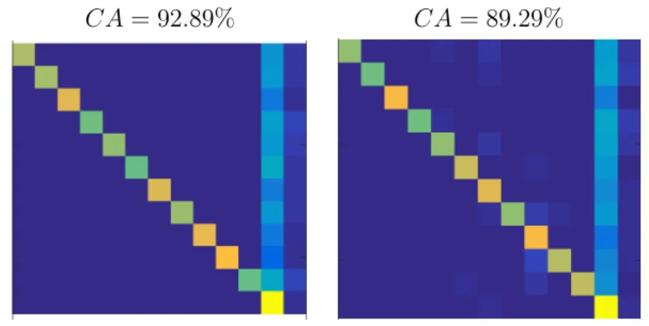
Prvi eksperiment preverja, kakˇsna je toˇcnost izboljˇsane metode. Ta eksper-iment je zelo pomemben, ker nam poda referenˇcno toˇcko za primerjavo os-talih rezultatov z originalnimi. Ugotovili smo, da ko na MSRC zbirki upora-bimo naˇso izboljˇsano metodo, doupora-bimo klasifikacijsko toˇcnostCA= 92,89%in zelo visoko mero napaˇcno pozitivnih primerov v razredu ozadja (F P R = 27,27%). Enak eksperiment smo izvedli tudi na VOC 2007 zbirki, kjer smo dobili klasifikacijsko toˇcnost CA = 89,29% in F P R = 19,27%. Predstavl-jeni podatki so ustrezna referenˇcna toˇcka, le da je mera napaˇcno pozitivnih primerov visoka. Ta problem smo poskusili reˇsiti v drugem eksperimentu.

Drugi eksperiment je preverjal, kakˇsen je vpliv praga za generiranje seg-mentiranih slik. Razliˇcen prag generira razliˇcno stopnjo razgradnje ene vhodne slike. ˇCe je prag viˇsji, potem dobimo precej majhno ˇstevilo segmentov, ki so veliki. ˇCe uporabimo majhen prag, potem pa dobimo veliko majhnih segmen-tov, kar je prav tako raˇcunsko zelo zahtevno; ˇse posebej to, kako bi od vseh

Originalna metoda Z ozadjem

CA= 78.70% CA= 92.46%

Figure 1: Ilustracija naˇse izboljˇsave. Modra barva predstavlja relevantni razred, v naˇsem primeru kravo. V originalni metodi poleg relevantnega razreda obstajajo tudi drugi razredi in razred krava je razˇsirjen zunaj toˇcnega obmoˇcja. Nimamo naˇcinov, s katerimi bi izraˇcunali, kakˇsna napaka je bila narejena zunaj oznaˇcenega obmoˇcja. V naˇsi izboljˇsani metod je napoved oˇcitna in vsebuje samo relevantne razrede, kravo inozadje. Vidna je tudi izboljˇsava klasifikacijske toˇcnosti.

podlagi pridobljenih rezultatov smo ugotovili, da je najboljˇsi prag t= 0,30. Tretji eksperiment preverja toˇcnost prenesenega znanja z ene zbirke na drugo. Imamo dva razliˇcna primera: (I)) ko prenaˇsamo znanje iz MSRC zbirke naVOC 2007 zbirko, (II)ko prenaˇsamo znanje izVOC 2007 zbirke na MSRC zbirko. V (I) primeru opaˇzamo zelo majhno mero pravilno pozitivnih primerov na vseh razredih, razen razredaozadja T P RI = 35,25%, in zelo vi-soko mero napaˇcno pozitivnih primerov v razredu ozadje F P Rbg_I = 53,47%. Klasifikacijska toˇcnost v tem primeru je CA = 83,11%, kar je slabˇse od referenˇcne toˇcke. V (II) primeru sta mera pravilno pozitivnih primerov in klasifikacijska toˇcnost malo viˇsja glede I primera T P RII = 37,39%;CA = 86,85%, in mera napaˇcno pozitivnih razredovozadjeje precej niˇzjaF P R_IIbg = 45,14%. Priˇcakovano je bilo, da smo dobili slabˇse rezultate zaradi morebitnih faktorjev, kot so: podobnost na podlagi prisotnih barv v sliki, svetlost, POV objekti na slikah razliˇcnih zbirk, podobnost objektov posameznih razredov in definicije ekvivalentnih razredov. V obeh primerih razred ozadje dominira v meri napaˇcno pozitivnih primerov, kar je vidno na Sliki 2. Poudarjena vrstica na desni strani matrik predstavlja razredozadje. Na podlagi rezultatov smo ugotovili da je bolje prenaˇsati znanje v II primeru kot je v I.

ˇ

Cetrti eksperiment preverja, kakˇsen je vpliv velikosti uˇcne mnoˇzice razreda ozadje. Meritev vpliva je bila narejena v zmanjˇsani podatkovni zbirki. Zmanjˇsali smo jo tako, da smo odstranili vse slike, ki ne vsebujejo pomembnih ano-tacij.Zmanjˇsani zbirki sta pribliˇzno 50% manjˇsi od originalne velikosti. V obeh primerih smo dobili slabˇse rezultate mere klasifikacijske toˇcnostiCA= 82,89%;CA = 83,00%. Mera napaˇcno pozitivnega razreda ozadje se je zmanjˇsala, mera povpreˇcnih napaˇcno pozitivnih primerov vseh razredov pa se je zviˇsala. To pomeni, da so se napaˇcno pozitivni primeri razprˇsili ˇcez vse ostale razrede, kar je slabo, saj ni mogoˇce napovedati, v katerem razredu naj bo naslednja napaka. Na podlagi rezultatov smo potrdili, da je prenos znanja iz I primera boljˇsi kot prenos iz primera II. S tem smo potrdili, da

Peti eksperiment zdruˇzuje obe zbirki in preverja, ali je kombinacija zbirk boljˇsa kot prenos znanja. Zdruˇzitev je bila narejena posebej za uˇcni in testni mnoˇzici, potem pa smo uporabili enako pripravo kot v prvem eksperimentu. Tokrat smo dobili klasifikacijsko toˇcnost na testni mnoˇzici kar je slabˇse tudi od prenosa znanja v obeh primerih. V tem eksperimentu so napaˇcno poz-itivni primeri ˇse bolj razprˇseni po ostalih razredih. Slabˇsi rezultati so bili priˇcakovani, ker ni bilo dovolj primerov v posameznih razredih, z ozirom na to, da je definicija razredov razˇsirjena z definicijami iz obeh podatkovnih zbirk. Ne glede na to pa razred ozadje ni veˇc dominanten, kot je bil pri prenosu znanja v tretjem eksperimentu, na raˇcun slabˇsih sploˇsnih rezulta-tov.

V sploˇsnem so rezultati vseh eksperimentov dovolj dobri, da bi lahko nadaljevali z obˇsirno analizo prenosa znanj z naˇso izboljˇsano metodo. V nadaljevanju bi lahko delali veˇc na hitrosti naˇse metode in preverjanju de-lovanja na veˇcjih podatkovnih zbirkah, ki imajo veˇc uˇcnih primerov, kar pomeni, da boljˇse generalizirajo svoje razrede.

CA= 83.11% CA= 86.85%

Figure 2: Matrike pravilnih in napaˇcnih razvrstitev iz drugega eksperimenta. Leva matrika predstavlja I primer, desna matrika II primer.

Introduction

At present time, building of robots for various use cases, such as [33, 37, 6], is very common. This is a fairly complex process, due to the fact that the robot is consisted of various modules, such as a navigation, sensing, manipulation, and a module that lets all the modules communicate between each other and thus make it intelligent.

These modules, at present time, are not entirely universal, i.e., they need to be adjusted for the purpose of the robot. And since we are designing robots to do various tasks, such as simple navigational robot, agricultural robot, space exploring robot, there are various levels of accuracy for specific tasks and it makes sense that they should be customized. The motivation for this thesis is a rescue robot, whose task is to navigate through an area which has been exposed to some kind of a disaster, for example an earthquake, fire, or post-flood ruins and create a map of the area. It must map where are all the victims of the disaster, and all the potential threats such as a parts of the building which are likely to collapse, fire which has not been put off yet, dangerous gases which are most likely going to light up, etc.

One of the modules which is a part of the system is the vision perception module, which is taking raw camera footage as input, process it, and make some conclusions based on the output. This system is in fact performing semantic segmentation of the raw images, it breaks the image into regions

and understands what each regions’ meaning is, is it an animal, or is it a building, or maybe a vehicle.

This thesis uses the approach introduced in [10] as a starting point. We explore the method, whose main problem is solving the texture representation problem, and how to make it as compact as possible for classification. We extend the approach by introducing a background class (Chapter 4). Our aim is to check whether it is possible to use this method as a part of an iterative learning process which includes both object and texture recognition methods. The learning process is consisted of finding an object in the image and classifying it in an object category. The categorized item’s texture is also classified. Both pieces of information are then used to check the likelihood of them being a pair and further improve the learning. For example, if there is a wooden table on the image and the detected object is a table then we would expect the texture to be a material of which the table is probably made of (wood, metal, plastic, etc.).

The design of the vision module of our rescue robot required a lot of training data which was not available to us, and we didn’t have time to label the data at our disposal. Due to this fact, our goal is to check whether it is possible to use this method to train a model which is going to generalise well enough its classes in order to classify the textures and objects with as little error as possible. We also analyse in depth the results obtained from the experiments.

1.1

Related work

Texture representation has been around for a long time, and [10] was cer-tainly not the first attempt to find an optimal solution. Since the textures consist of an extremely large diversity of visual patterns, the idea is to extract information from the textures locally and uniformly from the entire image.

There are the classical approaches to texture representation, which con-sist of a deterministic, hand-crafted1 algorithm for extracting local features

such as [47, 5, 12, 3, 35].

Lately, the focus has been set on features extracted from the convolu-tional layers of the Convoluconvolu-tional Neural Networks, as it has been presented in 2012 by Krizhevsky et al. [24] that significantly outperforms the hand-crafted algorithms. This motivated numerous research groups to build simi-lar models, specialized in various domains, such as [20], which transfers the domain of [24], which is trained explicitly for [13], to [16]. While doing so, they are reusing the pre-learned weights on the ImageNet dataset [13], and adapting them for the domain of [16]. Their approach is consisted of remap-ping class labels between the source and target domains, i.e., adjusting the neural network architecture and retraining it for the target domain. Another related approach is [31], which is introducing a framework for building ANNs and reusing already trained network parameters. This framework allows the community to break the neural networks into Lego pieces and customize them at will.

What is common for the previously listed approaches is that they are solely based on neural network customization. They are extracting image features from the convolutional layer, and use the upper layers of the net-works, i.e. the fully-connected layers, as classifiers. On the other hand, some of research groups discovered that extracting features from the image and use feature encoders used for building SVM models, such as in [10], is improving the model’s performance. This core concept is the basis of our work.

1_{The termhand-crafted is used to describe algorithms which are following a strictly}

1.2

Thesis layout

Chapter 1 states what motivated us to focus on the problem of semantic image segmentation. And introduces into the main challenges that we en-countered.

In Chapter 2 we discuss all the prerequisite methods that are used for successful semantic image segmentation. It includes the basics such as defi-nition of a digital image and a texture. It also defines what image features are, how they are extracted and encoded together. Finally, we explain what is classification and how we apply it in this case.

Chapter 3 contains a review of Artificial Neural Networks. We explain the basics of the ANNs, what is their background, how they are built, ex-plains the learning process and what types of ANNs there are, along with their application. This chapter also further explains how the Convolutional Neural Networks work, as they are one of the basic building blocks of the methods used.

In Chapter 4 we explain what transfer of knowledge is, what semantic segmentation is, and how [10] works, along with its main components for pre-segmentation of the images.

In Chapter 5 are laid out the experiments which were done on theMSRC [48] andPASCAL VOC 2007 [16] data-sets, the results along with their analysis.

Chapter 6 summarises this thesis by pointing out the main issues it re-gards, which experiments were done and the conclusions from the analysis of the experiments. It also motivates the future work of the thesis.

Texture recognition

Computer vision is a field of computer science which addresses automatic processing of images and videos. It is composed of acquiring, processing and analysing digital images and videos. This thesis is exploring a method for analysing of images. Its task is to recognize textures in images and its purpose is to provide semantic information about the structure of the images. This chapter is devoted to describing components of the method for texture recognition in a bottom-up fashion, describing what digital images are at the beginning and explaining how to discriminate between different textures.

2.1

Digital Images

The visual representation of something, e.g. a natural scenery, is called an image. Such images can be represented in a computer-friendly form, i.e. a form that a computer can understand, a binary representation. These images are calleddigital images. There are two types of representations of the images in the digital world, depending on whether they have a fixed resolution,raster images or not, i.e. vector images. We set our focus on raster images, as they have properties which are most suited for the particular problem that this thesis is reviewing (Section 2.1.1). Another reason why we should consider using only raster images is the fact that vector images can easily be rasterized.

2.1.1

Raster images

Raster images are a type ofdigital images with a fixed resolution. The main characteristic of this representation is that it is consisted of a finite set of elements, called pixels. Each pixel has its own value which represents its intensity. The intensity describes how bright the particular pixel is when the image is shown on, for example, a monitor or another medium.

Pixels are organised in rectangular matrices. There are rows and columns of pixel values and at any given time one can check the value of any partic-ular pixel. In other words, pointing to a specific patch of an image will yield a subset of pixel values of the image.

To represent coloured images in raster graphics there are a variety of models, which all have a common idea of representing the colours via multi-ple layers of pixel values. Each layer consisting pixel values for a particular colour channel. For example in theRGB (Red-Green-Blue) colour model each layer contains values for red, green and blue colour respectively. Each pixel has three intensities: red, green, blue. When all three pieces of information are combined together, with a mathematical formula, they output the final colour of the pixel.

Matrix representation of the images is actually a set of pixel values. Matri-ces are suitable if we would like to further group them based on the similarity of their value, distinguish between contrasting values and where they are lo-cated at (neighbourhood). This allows us to build clusters, or super-pixels, which can further have some semantic meaning. In contrast, vector represen-tation does not allow us to this particular thing, since in this represenrepresen-tation the all the values are generated from curves, which are not necessarily as simple as in a set of numbers.

2.2

Texture

A variety of definitions for textures exist and because of this D. Forsyth, in his book [18], wrote: “Texture is a phenomenon that is widespread, easy

to recognise, and hard to define”. In our case the most relevant definition is that a texture is a subset of pixels which are repeatedly recurring in a neighbourhood. The repeating pattern is called a texton. The texton is most frequently a small object which is constantly repeating throughout an image patch, for example a close-up image of a leaf represents the object of the image, but when the object of the image is a tree, a leaf is merely a repetitive pattern that is recurring throughout the foliage of the tree.

There need not be strictly one texton, there can be multiple textons, or multiple textons which are generating other textons using a stochastic functionf [10].

Very often a material is characterized by its texture, which has a repeating pattern that makes the object distinguishable from all of its surroundings. The application of textures is correlated to the materials. Many times the goal is to robustly detect different textures in order to determine what kind of objects are there in the image, what they are made of, what is the relationship between the objects on the image etc.

The correlation between textures and materials cannot be relied upon always. There are objects of the same category but made out of different materials. For example a table can be made of wood, and it can also be made out of plastic or various metals and metal alloys. In the end all of those objects are tables, just made out of different materials.

Often it is required to compare distinct patches of images which contain possibly unassociated textures. To do so we need to represent each texture’s properties which can be presented formally with various feature descriptors.

2.3

Image Features

To outline the characteristics of image patches we use local image features. Each feature has to be distinguishable in the image regardless of viewpoint or illumination, has to be robust to occlusion - must be local and must have a discriminative neighbourhood [47].

There are various applications of image features, such as matching in-stances in multiple views, epipolar geometry or homography, photo tourism, panoramic mosaic, query by image etc. In the scope of this thesis we are bounded by the application of describing the textures of image objects and discriminating between different texture classes.

Image features, essentially, are extracted from regions of the image that contain image-specific characteristics such as edges or corners of texton fea-tures. We are interested in these regions in the task we are dealing with, and that is why we are computing the features on them, in this case we want to discriminate between different texture classes.

2.4

Feature descriptors

A feature descriptor is a vector which is obtained by an algorithm in order to describe the image region which is of interest for further computation. These image regions represent a variety of materials, i.e. objects, and are located throughout the image. The feature descriptor encodes the image patch to make it distinguishable from the rest of the image features. In ideal cases, the algorithm is invariant to image transformations, such as translation, scaling, rotation, outputting an almost identical vector under various such transfor-mations. Depending on the technique used to obtain the feature descriptors, they can be either hand-crafted orlearned.

2.4.1

Hand-crafted descriptors

Hand-crafted descriptors are obtained by using a deterministic algorithm to describe the image features. Such descriptors use various techniques to achieve robustness to misalignment, illumination, blur, compression, as well as it has to be efficient - ability to be computed on-line i.e. in real time and use as little memory as possible [47]. Examples of such descriptors are Scale Invariant Feature Transformation (SIFT) [5], Histogram of Gradients (HoG) [12], Speeded Up Robust Features (SURF) [3], Local Binary Patterns

(LBP) [35]. In order to be able to compare how the hand-crafted and learned features are formed, we briefly explain SIFT in the following section.

2.4.1.1 Scale Invariant Feature Transformation (SIFT)

SIFT [5] is a very popular and commercially widespread feature descriptor since it is more robust then most of the rest descriptors which makes it very efficient. SIFT features are formed by computing a 16×16 window around the given point of interest (key point). At each value of the window the im-age gradient is calculated at the appropriate level of the Gaussian pyramid at which the point was detected and smoothed over a few neighbours. The window is divided in 4×4 quadrants, and for each of them a histogram of oriented gradients with 8 neighbours is formed. The final output of the de-scriptor is a a horizontal stack of each histogram, yielding a 128 dimensional vector.

2.4.2

Learned features

Learned features are extracted using a machine learning method, such as convolutional neural networks (CNNs) which are used in our work. According to [24] they outperform hand-crafted features. Each layer in a CNN can be interpreted as a functionφK(x),xis an input image. The output at theK-th layer is then a composition (φ1(x)◦φ2(x1)◦· · ·◦φK(xK−1), wherex1, . . . , xK−1

are outputs of each layer) of all the layer functions and is a descriptor field xK ∈ RWk×Hk×Dk of the input image. Where Wk and Hk are width and height of the field andDk is the number of feature channels [10].

In [10] the last convolutional layer is used to obtain the learned feature. This approach is used in this thesis, as [10] have proven that it is state-of-the-art while researching the field.

2.5

Feature vectors

Feature vectors are a compact way of encoding image features. Each value of the feature vector has its own meaning, and looked at the whole vector it represents a numerical representation of the object that is being encoded, in computer vision, many features are combined (encoded) together in a single vector, yielding the equivalent of all the image features, in whichever form they may be.

The method discussed in this thesis uses Fisher vectors for encoding the image features extracted from CNNs. In Section 2.5.1 they are briefly de-scribed.

2.5.1

Fisher Vectors (FV)

Fisher Vectors serve as an image representation. In the method discussed in this work they are obtained with pooling local image features from the provided CNN. They are a special, approximate and improved case of the general Fisher Kernel framework [46]. The derivation of the Fisher Vectors is available in [46].

Fisher Kernels [34] are a mixture of generative and discriminative ap-proaches in classification. All the mathematical details for Fisher Kernels are available in [34].

2.6

Classification

One of machine learning’s core problems is classification. It is the problem of categorizing items into their correct category, for example categorizing an image of a cat into the category of cats. This is being done with a supervised technique, i.e., the methods for classification are divided into two basic steps: training and testing.

Training is the step when the method learns about the given data. There are two key pieces of data that is provided: input of the method and the

correct output. The data should be evenly distributed for each category, so that the method is not biased towards a subset of the categories. Once the method has learned all of the training data it is ready for the testing stage.

The testing step is used to expose the method to new, previously unseen, data. This step provides insight about how well the method is discriminating between different categories. For example, if we provide the method, dur-ing testdur-ing, a picture of a breed of cat which is not present in the traindur-ing samples; based on the output of the method we can conclude whether it is generalising the category of a cat well (it outputs that it is a cat), or that it is not generalising well and it can be further improved by either providing more training data or tweaking the parameters or changing the method altogether. There are many such methods, varying in their complexity. Such meth-ods are: logistic regression, Naive Bayes classifier, Support Vector Machines (SVMs), K-Nearest Neighbours, Decision Trees, etc.

2.6.1

Support Vector Machines (SVM)

One of the most wide-spread tools for solving supervised learning tasks are SVMs. They are used for building models for solving both classification and regression tasks. SVMs take feature vectors as input and try to represent them in a feature space. The goal is to find a hyperplane that separates the data and minimizing the classification error.

For example, if we have 2-dimensional features, such as presented in Fig-ure 2.1, the data is linearly separated, i.e. there exists a line (hyperplane) which can clearly divide the 2 classes present in the data-set. Similarly, when the features of a higher dimension we try to do the same thing, find a hyper-plane that divides both classes.

Since SVM represents the training examples in a feature space and tries to fit a hyperplane which is separating them best, it is a deterministic approach to solving the classification problem. There are techniques of retrieving prob-abilities, such as [49], based on the distance from the decision boundary.

of a technique calledkernel trick [45] which allows it to achieve flexibility and expands it to non-linear spaces, leading to non-linear decision boundaries.

More details about SVM and the mathematical approach can be found in [11, 45, 4].

Figure 2.1: A simple example of a linearly separable data-set. There is an infinite number of lines between both of the classes. The SVM method chooses the one which has the maximal distance to the nearest training samples. This is the case of optimal classification and it makes sense because when the data-points are separable they do not mix, and it can clearly seen on this visualisation.

Artificial Neural Networks

Artificial Neural Networks (ANN) are one of the pillars of this thesis. The goal of this chapter is to introduce the Convolutional Neural Networks (CNNs) and we will achieve that with a short introduction into general artificial neu-ral networks: what they are, what they are consisted of, basic concepts and algorithms that are used generally and what are the most common types of artificial neural networks used and for what purpose they are used.

3.1

General overview

Inspiration for the neural networks are biological neurons, whose structure is described in Figure 3.1. The first idea was to model how the biological neuron works, but it turned out that this structure can also be applied in machine learning to detect patterns and it achieves really good results. This is where the paths of biological neurons and mathematical models of neurons diverge. Modern implementations of neural networks do not have much in common with the real models of neural networks, and there are only speculations that there are similarities between them.

In Figure 3.2 is presented the computational model of a neuron. A single neuron is interpreted as a linear classifier. It has the capacity tolike ordislike some regions of the linear space.

3.1.1

Activation functions

Activation functions are used to model a neuron’s firing rate1. Essentially, they get the dot product between the inputs and weights as input (a scalar), perform a sequence of mathematical operations on it and pass the output further up the network. Here is a list of commonly used activation functions:

Sigmoid activation function is the historically most used activation function. Its equation is σ(x) = ₁₊1_e−x, where x denotes the input of the neuron, visually presented in Figure 3.3. It is sensitive to really big inputs (it outputs ≈ 1) and really small inputs (it outputs ≈ 0), and it is why it is very easy to interpret it: if the output is ≈ 0 the neuron does not fire. This means the neuron does is not responsive to that part of the space, and vice versa if the output is ≈1 the neuron fires, i.e., the neuron is responsive to that part of the space. Even though it is very simple to understand the output, in practice with deep neural networks the sigmoid function is not preferred because it causes problems further on in the computation of neural network because it saturates the gradient eventually ’killing’ it; this happens when the output is near both maximal and minimal value because the gra-dient is≈0, which means that when doing back-propagation (3.2) whatever value is being passed down through the saturated neurons will be eradicated leading to a stop of the learning capabilities of the network. Another reason why it is not preferred is because the output is not zero centred. This influ-ences the learning process. When all the values of the neuron are positive then the gradient is also either positive or negative, which may lead to an undesirable update of the weights. These problems do not occur in ’shallow’

1_{Output in biological neurons is dependent on the strength of the signal in the input.}

When the signal is above the predetermined threshold we say that the neuron has fired. These outputs are distributed though time, but since we are not interested in the particular timings when they occurred, the frequency of spikes along the axon is the unit we measure.

networks, that is why, historically, the sigmoid function was so popular. Tanh activation function is shown in Figure 3.4. It has a similar shape as the sigmoid function, but unlike it, tanh outputs real values in the range of [−1,1], so it removes sigmoid’s issue of the values not being zero-centred. Nevertheless, it still has the problem of saturating the gradient. In practice, tanh is always preferred to sigmoid.

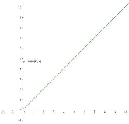
Rectified Linear Unit (ReLU) activation function is shown in Figure 3.5 and its equation to compute isf(x) =max(0, x). ReLU sets all the negative values to 0 and leaves the positive values as they are. ReLU is linear, so it is not saturating the gradient on one side, but there still is a problem when the values are negative, as the gradient is equal to 0, and deactivating a certain part of the network. Nevertheless, [24] showed that it accelerates the learning, and in their case by a factor of ×6. It is very easy to compute: it is required to threshold a matrix at 0.

3.1.2

Architecture

Neural networks are represented as acyclic graphs where sets of neurons are connected between each other. Each set of neurons denotes one layer of the neural network and they usually do not have connections among themselves. Each layer is connected only to the neighbouring layers. Layers that have all possible connections between pairs of neurons are called fully-connected layers and are very common in practice, but they are not the only kind of connections. The graphs are acyclic so that the input will not cycle forever in the network. Each neuron at one layer has the same activation function. Illustrations of neural networks are shown in Figure 3.6.

Layers can have different number of neurons and different number of connections to the neighbouring ones. The number of layers and neurons per layer define the network’scapacity. The more layers and the more neurons per layer, the greater the capacity of the neural network. The capacity denotes

the amount of representable functions in the network and the amount of precision of each functions’ representation, the more capacity it has, the more expressive the network is. Drawbacks of having greater capacity is exponential growth of the training time, and it can easily overfit the data. This produces a network which can never be used for testing purposes because if the test cases are not similar to the training data, it will perform poorly.

The network has an input layer, which is not taken into account for the final number of layers. The final layer is called the output layer. The layers which are between the input and output layer are called hidden, since outputs from individual layers are rarely used and we often are not explicitly interested in which state they are in.

Neural networks are organized in layers in order to achieve efficiency in calculation of the network values. The layers also allow usage of vector-matrix operations with which multiple values can be calculated at once.

3.1.3

Forward pass

The forward pass is done by passing the input through the network and getting an output. To get the output, the input is propagated through the network, gradually being transformed by each layer through the dot product with the weights of the connections and its activation function up to the net-work’s output. The output can be a single scalar value or a vector of values, depending on the output layer layout.

A simple neural network is presented in Figure 3.6. An example compu-tation of a forward pass: suppose that there is no bias, the weights of the first layer are stored in matrix W1 with size 5×3, where each row presents the weights of a single neuron. The input for the activation function y1 = σ(z)

of the hidden layer is calculated as z =W1x. The same process is repeated

for the second layer, except W2 is of dimensions 2×5 and the final output is

a 2-dimensional vector. An example application of this kind of a network is a logical function such as AND, OR, XOR, NAND.

Figure 3.1: Biological model of a neuron [21]. A neuron’s cell body is made up of: nucleus, dendrites, axons. Impulses are carried into the nucleus via the dendrites where they are accumulated and as soon as there is enough charge, it is transmitted through the axon out of the neuron. Neurons are connected via synapses to the other neurons’ dendrites.

Figure 3.2: Mathematical model of a neuron [21].The mathematical model is consisted of the same core elements as the biological model. Except that it’s a deterministic model and all steps are predetermined. Output signals are carried out of the neuron by the axon (x0), and they interact with the dendrites of other

neurons multiplicatively (x0w0), weighted by the synapse strength (w0). There

can be multiple input dendrites into a neuron, so all of the reactions are summed up, which is the dot product (w·x =wTx) between the weights of the synapses (w) and the input signal from the axon (x). If the sum is above a given threshold we say that the neuron fires by sending a spike along the axon (output). Synapse weights are determining how much influence does one input have. The weights can be learned through a technique called back-propagation (see Section 3.2) and it allows the neural networks to be adaptive to their input/output in the learning phase. The calculated sum is an input to an activation function (described in Section 3.1.1).

Figure 3.4: Visualisation of the tanh(x) activation function.

Figure 3.6: Example of neural network architecture [44]. In this example the network has 2 layers, 1 hidden layer and an output layer. The layers are fully-connected, i.e. there are connections between all the neurons at each layer.

3.2

Back-propagation

An essential part of a neural network’s learning is the back-propagation (or simplybackprop) algorithm, which allows the information of the cost2 _{to flow}

backwards through the network. Its purpose is to compute the gradient of the cost function and propagate the error which was made by the forward pass [29]. It is very important to stress out that backprop is not the learn-ing algorithm the network is uslearn-ing, but merely a method of calculatlearn-ing the derivatives in the network which is exploiting the chain rule of derivatives.

Neural network’s output is interpreted as a composition of functions: f1(x0)◦f2(x1)◦ · · · ◦fN(xN−1), N being the number of layers in the neural

network. Functionsf1(x0), . . . , fN(xN−1) are the activation functions of each

layer in the network. With this being said, calculating the derivatives of every single neuron is a fairly trivial task. Recursively walking back through the layers down to the input layer of the network and applying the chain rule. A neural network can also be interpreted as a bigcomputational graph[30]. Each edge has its own weight, which is influencing the value being propagated through it. Each vertex has an activation function, which is non-linearly changing the input value. A computational graph is very convenient because it allows granulating very complex computations into smaller ones, which are very easy to compute.

Computational graphs can also be applied to calculating derivatives: cal-culating the derivative of a very complex expression is very hard, but if you divide it in tiny pieces it is manageable. This is where the advantages of the chain rule are applied.

An example computation is shown in Figure 3.7.

2_{The cost is calculated by a cost function (E). It represents the degree of fit to the}

data [27]. The learning process wants to achieve as little cost as possible and achieve good results which will not result in overfitting the data.

+ ? x 6 -5 y -2 -5 z -5 4 q 4 -5 f -20 1

Figure 3.7: An example of how the back-propagation algorithm works. The values above the lines are the values calculated after the operation is done, and the red values underneath it is the gradient at that point. So, the multiplication (or division) is just rotating the values, and the addition (or subtraction) is distributing the value of the gradient. While themaxoperation, is routing the gradient to the maximum value, ignoring the rest of the inputs.

3.3

Learning process of an ANN

Once the gradient in a graph node has been calculated, there are various strategies on how to update the parameters to achieve the fastest convergence of the network with minimum amount of error. Such optimization methods are [21]:

3.3.1

Stochastic Gradient Descent (SGD) [28]

• Vanilla updateis simply subtracting the linear combination of the learn-ing rate hyperparameter3 _{and the calculated gradient from the weights.}

Equation (3.1) demonstrates how it is calculated.

wt+1 ←wt−α∇f(wt) (3.1)

3_{Hyperparameters are metrics used by the machine learning algorithm which are set}

• Momentum update is influenced by physics. For example, if the ob-jective is to reach the end of a canyon-like (steep walls on the side, and a shallow ravine that leads to the objective point, the optimum) structure, SGD is most likely to approach the ravine very fast and then cycle across the steep sides, as it gains the biggest values there rather than across the ravine. This effect can even force the SGD to converge in a local optimum, which leads to suboptimal solutions in the long term. By adding the momentum we prevent this effect. It pushes the objective across the ravine faster:

vt+1 ←µvt−α∇f(wt) (3.2)

wt+1 ←wt+vt+1 (3.3)

Where v is initialized at 0 and µ ∈ (0,1] is another hyperparameter of the network, momentum, which controls how much influence has the momentum. Its typical value is 0.9, but it is often set at 0.5 at the beginning and then annealed to 0.9 later on. The purpose of the momentum update is for the parameter vector to build up velocity in the direction that has consistent gradient [21].

• Nesterov’s Accelerated Gradient (NAG)[41], unlike the normal momen-tum update, calculates the gradient of the function one step ahead in time, i.e. for the actual step that is going to be made with the update. This clever trick allows faster convergence of the learning process at no extra cost. The altered equations for the Nesterov’s Accelerated Gradient:

vt+1 ←µvt−α∇f(wt+µvt) (3.4)

3.3.2

Second order optimization methods

If working with small amount of data, then it would make sense to take advantage of second order optimization methods, which rely on Newton’s optimization method. The core idea is to iterate:

x←x−[Hf(x)]−1∇f(x) (3.6) whereHf(x) is a Hessian matrix [citation needed] with second-order partial derivatives of function f, while ∇f(x) is the same gradient term from SGD. It allows a more efficient update of the weights, since the Hessian matrix carries information about the local curvature of the loss function. It also re-moves the need of any additional hyperparameters, which is very convenient. Unfortunately it is very impractical because building the Hessian matrix and especially inverting it is almost impossible in practise. The dimensions of the matrix can easily go above 1000000×1000000 which is very difficult to store in RAM memory [21]. There are alternative approaches which are estimating the inverse of the Hessian matrix, such as L-BFGS [26].

3.3.3

Per-parameter adaptive learning rate methods

These methods are different from the rest of the described ones because they express the gradient per parameter, as opposed from the previous methods which all apply the same gradient to all the parameters. A list of most widely spread methods:

• Adagrad [14] is an adaptive learning rate method, it is characterized by Equations (3.7) and (3.8), C ←C+∇f(x) (3.7) x←x−α√∇f(x) C+ε, ε≈10 −6 (3.8) where C is a vector of the same size as ∇f(x), initialized at 0. Down-sides of Adagrad in its usage in deep learning is that a monotonic

learning rate(α) usually proves too aggressive and causes the learning to stop too soon.

• RMSprop[42] is an upgrade of Adagrad update which is only controlling how aggressive the monotonous learning rate is. The equations are:

C ←υC+ (1−υ)∇f(x)2 (3.9) x←x−α√∇f(x)

C+ε, ε ≈10

−6 _(3.10)

In the equations above, υ ∈ {0.9,0.99,0.999} (typically) is a hyperpa-rameter. In this case, C is leaky, it forgets previous values over time, thus yields adaptive parameters, but unlike Adagrad it doesn’t make them monotonically smaller.

• Adam [22] tries to combine both momentum and RMSprop, the sim-plified equations are:

m ←β1m+ (1−β1)∇f(x) (3.11)

v ←β2v+ (1−β2)∇f(x)2 (3.12)

x←x−α√m

v+ε (3.13)

in this case recommended values of the hyperparameters β1 = 0.9,

β2 = 0.99 and ε = 10−8. At the time of writing the thesis, this is the

recommended method for optimizing the parameter updates. Further details are available in [22].

3.4

Types of ANNs and their application

There are a lot of different types of ANNs, differing in their architecture, activation functions and data that are trying to model. To get the idea of what kind of ANNs exist, and what they are used for, we briefly describe here some of the most used ones:

• Recurrent Neural Networks(RNNs) These networks are non-linear dynamical systems that map sequences to sequences. Modelling se-quences requires their architecture to be rather unconventional with regards to what was previously stated, as there are connections between neurons at the same layer. This property makes them very difficult to train due to their non-linear iterative nature. Very little changes in an iterative process can compound and result in very large effects many iterations later. This is known as ”the butterfly effect” [40]. Meaning that the derivatives of the loss function can be extremely large to the activations of the hidden layers at earlier time, making the loss function sensitive to very small changes, so it becomes discontinuous (vanishing gradient problem).

• Radial Basis Function Networks (RBFs) are commonly consisted of an input layer, hidden layer and an output layer. So they are not deep networks and they are characterized by radial basis activation function of their hidden layer. A radial basis functions are used for approximation of other functions. Their form is showin in (3.14),

φ(x) = exp − kx−wk 2 σ2 (3.14) where σ is the activation strength parameter [43]. RBFs are used in regression problems, as they are particularly good at approximating other, unknown functions. Such applications are in data forecasting, market analysis, weather, load of electricity for a city [2].

• Convolutional Neural Networks (CNNs) are further discussed in Section 3.5. They are mostly used in computer vision to perform object detection and recognition, semantic segmentation.

3.5

Convolutional Neural Networks (CNNs)

Convolutional neural networks are specialized for dealing with data that can be represented in a matrix form, such as images, that is why they are suit-able for this thesis. They are a type of neural networks which useconvolution (further discussed in Section 3.5.1) instead of matrix multiplication in at least one of their layers [19].

They are characterized by having 3D volumes of neurons. The neurons in such a neural network are arranged into three dimensions: width, height, depth4(illustrated in Figure 3.8). Each layer of the CNN transforms its 3D volume input using an activation function which might have learnable pa-rameters and/or hyperpapa-rameters to an output 3D volume [21]. The trans-formations might cause the 3D volume to change its size.

A typical input is an image with dimensions W×H×D(width, height,

Figure 3.8: Visualisation of how the neurons are arranged in 3D volumes. depth), with depth denoting the number of colour channels of the image. For example CIFAR-105 images have dimensions 32×32×3, so they are 32

4_{not denoting the depth of the network}

5_{CIFAR-10 is a dataset consisted 60000 images with dimensions 32×32×3 divided}

pixels wide, 32 pixels high and have 3 colour channels. Having a 3D volume as input means that they are also outputting a 3D volume output, so in the case of CIFAR-10 the output is in the format of 1×1×10. This means that the network has reduced the images into a vector with 10 values, denoting the classes of the data set.

3.5.1

The convolution operator

Convolution is a mathematical operation, defined by the Equation (3.15). s(t) = (x∗w)(t) =

Z t

−∞

x(a)w(t−a)da (3.15) The operation is defined for any functions for which the integral is de-fined [19]. In probability theory [32], convolution is applied to determine the probability density distribution of sum of n mutually independent ran-dom variables X1, . . . , Xn.

Let us consider a simple case with two rolling dices. Let the outcome of the first dice be the random variable X and the Y of the second one. Their distribution is f(x) and g(x) respectively, and since we are throwing dices, they are both discrete probability distributions. If we want to deter-mine what is the probability of getting a sum of both rolled dices equal to 6, we have to sum the probabilities of rolling all the possible variations, i.e. calculating:

f(1)g(5) +f(2)g(4) +f(3)g(3) +f(4)g(2) +f(5)g(1) = 5

32 (3.16) If we apply the rule of discrete convolution which takes the form of:

s(t) = (x∗w)(t) = t

X

a=0

x(a)w(t−a) (3.17) in this particular case, we get:

s(4) = (f∗g)(5) =

5

X

a=0

which is exactly what we previously wrote in 3.16.

Regarding convolutional neural networks, the discrete version of convolu-tion (Equaconvolu-tion 3.17) is being used, as the data is discrete into integer values of each pixel of the images. Where we refer to x as the input (I) and w as the kernel (K), while the output is being referred to as the feature map [19]. Since the input to the CNNs are images, the convolution needs to be expressed with two dimensions, as:

s(t) = (I∗K)(i, j) = X m

X

n

I(m, n)K(i−m, j −n) (3.19) Convolution has the commutative property, expressed as:

s(t) = (K∗I)(i, j) = X m

X

n

I(i−m, j −n)K(m, n) (3.20) It also has the associative, distributive properties, expressed in a similar manner as the commutative property. What is important to point out is the property of translation invariance of the convolution. Essentially, if the function is translated by an arbitrary value, it doesn’t affect the final output of the convolution. In computer vision this means that no matter where the blob is in the image, if the current kernel can detect it (for example kernel for detecting edges), it will be detected no matter where it is located in the image.

3.5.2

Architecture of a CNN

CNN’s architecture is usually consisted of multiple layers of neurons and, as discussed previously, each layer has its own activation function. Most common types of layers used in a CNN are:

• Convolutional layeris the core building block of a convolutional neu-ral network [21]. Its parameters are actually learnable filters that are used for convolving the image, during the training, they learn to detect features in the image, such as edges, blobs, colour patterns on the first layer, and more complex features, such as honeycombs, in the deeper

convolutional layers. The filters are small spatially (they do not have connections to all neurons from the previous layer). This characteris-tic is controlled by the receptive field hyperparameter of the network. Each filter covers the entire depth of the image (every colour channel), and slides across the entire image. Following the assumption that if a feature is useful to calculate for one position, it is also useful to have it for another position as well. Thus sharing the parameters with other neurons seems like a very nice idea. Sharing the parameters means that each depth slice of the output volume of neurons has only one set of parameters (illustrated in Figure 3.9).

To control the output volume of the layer, three parameters are used: depth, stride and zero-padding. Depth denotes how many different fil-ters we would like to have in the output. As mentioned before, each depth slice is a filter. Stride controls how many pixels the filter is moved while convolving, it is typically set to 1, but there are excep-tions. Zero-padding controls the spatial size of the output, this is due to the fact that convolution changes the size of the input on its output, and adding zeros on the edges preserves the size of the output.

• Pooling layer is used for reducing the number of parameters in the network, by reducing the spatial size of the representation. This helps preventing the network from overfitting. Most common function used for pooling ismax, which only lets the maximum response in a provided patch to continue through the network.

• Fully-Connected (FC) layer These layers have connection with ev-ery neuron from the previous layer, as often described the simplest case of artificial neural networks (see Section 3.1.2 for more details) . The layers are usually ordered in a predetermined pattern. First, there is a convolutional layer, then a layer with a simple ReLU activation function, followed by a pooling layer. These three layers ought to be repeated a several times, representing the feature extraction from the images. Then they are

followed by a fully-connected layer, which is the actual classifier, further reducing the output to a probability distribution for each class, as previously described in Section 3.1.2.

Figure 3.9: Visualisation of trained convolutional filters of the VGG-16 CNN [9]. These images represent a sample from the 512 learned filters of the fourth convo-lutional layer.

Our approach

The aim of our approach is to test whether it is possible to use transfer of knowledge (TOK), discussed in Section 4.1, to transfer knowledge between different dataset in the field of semantic image segmentation. For this pur-pose, we used the deep filter banks [10] method as a starting point. During the testing, anomalies occurred which influenced the overall performance of the method, these are discussed in Section 4.3.

4.1

Transfer of Knowledge

In general, when a new approach is being developed the data used to prove whether it works or not is hand-picked to present the best samples, in order to prove the method worthy of further improvements. It is only when the developed method is tested in the real world and with real data, which is quite often inconsistent in regards to what we have previously worked with, that we discover that what we saw in the laboratory is not what we get in the real world [25].

The idea behind domain transfer is reusability of already gained knowl-edge. For example, if there has been developed an intelligent system for detection of score-changing events in a tennis singles match, and we would like to adapt this system to work for a badminton doubles match [17]. We,

on the other hand deal with the lack of data in the similar manner as [38]. In our case, there is lack of labelled data. The solution is to check the performance of two datasets which only have overlapping classes of objects and what is the performance when the knowledge obtained through training is simply transferred to the other dataset’s domain.

As it is described in [38], we did encounter similar problems, for exam-ple same class of objects, but different viewpoint, or alternative types of the same object. The analysis of the experiments and problems we encountered are further discussed in Chapter 5.

4.2

Semantic segmentation

To try to solve semantic segmentation, we first need to know what segmen-tation is. There are two perspectives of how we can approach this problem: (1) the process of breaking the image into regions and structures, such as circles, various polygons; or (2) grouping pixels into larger sets, and again, making up various kinds of structures, called super-pixels.

Semantics add another layer of abstraction of the generated regions, i.e. understanding. It is also referred to as image understanding, as it provides us with additional information about the image, what kind of objects are there in the image. This can be further used for detection of the interaction between the objects on the image and generation of image captions. The segmentation process generates the segments, and semantics add the mean-ing of those segments in the image.

To explore semantic segmentation we refer to the work by Cimpoi et. al [10]. To sum up this method, it uses CNNs to extract image features from the images, encodes the features in one large feature vector and uses SVMs to classify the output results. As for the testing phase it uses an additional method for pre-segmentation of the input test images. The following sections describe the methods in more details.

4.2.1

Image Segmentation Proposal

In order to add semantics to the image, we need to have some region pro-posals, i.e., segments of the image which have a probability of containing an object of interest. There are various techniques for breaking the image into regions, such are [7, 15]. In the work done in this thesis, we used a state-of-the-art method by Arbel´aez et al. [36].

The method by Arbel´aez et al. [36] considers as an input an image, for which various type of local contour cues have been extracted, such as bright-ness, colour and texture differences; sparse coding on patches; and structured forest contours. The contour cues are then globalized independently with their fast technique for eigenvector gradients, and then construct a UCM based on the mean contour strength. This is done for each scale, and then the gathered information is aligned, as to preserve the locality of the infor-mation in the image, the location of each object. Then to choose from the best boundaries of the objects, a binary boundary classification problem is defined which combines all of the features in a single probability of bound-ary estimation. The output of the method is a UCM (see Section 4.2.1.1). Further details for this method can be found in the original paper [36]. 4.2.1.1 Ultrametric Contour Map (UCM)

Ultrametric Contour Maps [1] are a rather useful tool for region proposal generation. Let S={S∗, S1_{, . . . , S}L_{} be a set of segmentations of the image} which partition the domain from fine super-pixels (S∗) to a partition that represents the whole domain (SL) and every new element is the union of all the previous elements. The domain is presented in a hierarchy. Each levelSi has a real-valued indexλi. Using the indices, the hierarchy can be presented as a dendrogram. In terms of the UCMs, applying the thresholdλi will yield the segmentations from Si _{set. For example, if there is a car on the input} image, let theSi_{−th partition contain the wheels, the body of the car, and} the windows of the car separated, the next partition, on theSi+1−th level, will contain the entire car segmented as one piece. That means that the lower

the threshold is, the more segments are going to be generated.

4.2.2

Deep Filter Banks (DFB)

Deep Filter Banks [10] is based on texture recognition. One of their research points, which is relevant to our work, is to test multiple types of image features, techniques of pooling them together, and building a classifier for discriminating them, as well as applying it to semantic segmentation. From all of their findings, the most suitable for our work is the usage of CNN fea-tures, encoded with Fisher Vectors and building a model with SVM.

The [10] method, by the standard principles of machine learning, is di-vided in a training and testing stage. During the training stage, image fea-tures are acquired from the images using the ground-truths provided for the images (Section 4.2.2.1). Next, the features are encoded into a feature vec-tor (Section 4.2.2.2). Finally, the feature vecvec-tors are fed into a classification algorithm (SVM), to build a model, which is going to be used for classifying the testing images (Section 4.2.2.3).

The testing stage is somewhat different than the training stage owing to the fact that testing on the ground-truth data makes no sense. The [10] method does not break the image down into regions, it is instead focused on classifying them, thus we need the method described in Section 4.2.1, which provides them, and they are regarded in the same manner as the ground truth is in the training stage.

It is very likely that the pre-segmentation method generates much more regions than there are in the ground-truth, so during the testing stage, each of the regions is being classified, and as some neighbouring patches are dedi-cated to the same class, they are merged together. Nevertheless, the regions are divided by a 1 pixel border, as to be possible to distinguish between different regions. These borders are not regarded while calculating the final statistics and measuring the performance of the experiments.

4.2.2.1 Image features

The [10] method uses learned image features (as discussed in Section 2.3). The features are extracted from the last convolutional layer of the provided CNN (CNNs are further discussed in Section 3.5). In general, the DFB method can work with any arbitrary CNN, such as are the popular models of ImageNet [24], VGG-VD [39]. For our work, we used the VGG-M [8] model. Learned features are gained from a non-deterministic algorithm, and thus have the properties which every stochastic process has, i.e. they are unpre-dictable. In our case the unpredictability is good because we might never design features with properties which are extracted from a non-deterministic algorithm. As much as the unpredictability is good, using it can backfire on us. If the learning process is not modelled well, and the parameters are not well tuned, it can be led in the wrong learning direction. In this case making the overall result of the texture classification incorrect.

4.2.2.2 Feature encoding

Once extracted, the features are in a form which cannot be used properly for the upcoming classification task. That is, a matrix consisted of all the component of the raw features extracted from the CNN [10].

In order to convert them in the appropriate form, features for a particular region are encoded into a feature vector (they are discussed in Section 2.5). In order to preserve as much data as possible, so that the classification can be performed most accurately, the features are encoded into a Fisher vector, which preserves up to second-degree statistics for its input.

4.2.2.3 Texture classification

Information encoded into Fisher vectors is supplied to an SVM classifier, which is excellent for this task due to the fact that it works really well with high dimensional data, such are the Fisher vectors in this case, which can have more than 65000 features (details provided in [10]).

Since we are trying to classify objects, i.e. textures, which can be a part of more than two classes, as specified in the used datasets, the SVM classifier is trained as one-vs-rest. Meaning that there are multiple SVM classifiers trained, and the highest score of them all is the final class of the tested item (image patch in this case).

4.3

Our contribution

As shown in [10], the DFB method set the state-of-the-art standard for texture-descriptor accuracy. Nevertheless, its performance is measured on the labelled parts of the ground-truth only. We are also interested in how the method handles the areas which do not belong to any of the provided classes.

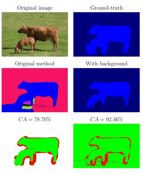
To check the performance of the original approach [10] we did a pre-liminary analysis. The classification of the ground-truth is performed with remarkable accuracy and even provides better precision to the contours of the object of interest than the provided ground-truth. However, since each region has to be classified during testing, the regions from the ground-truth which are unclassified, i.e. no object of interest is present, are forcefully classified in some of the classes. The worst case for these regions is to be classified as the target class (illustrated in Figure 4.1), affecting the overall accuracy of the method.

In our case, we needed an output which will provide us the classes of image regions belonging to known categories as accurately as possible. We also needed an output that will ”filter out” all regions belonging to unknown categories. As there is no way of knowing where are known and where are unknown objects in any given image, introduction of a background class is the best known solution. Thebackground class is designed to group together the regions which are not of interest, i.e., do not belong to any known class. Provided image labels are not covering the entire image, therefore this solu-tion allowed us to have a lot of training data for the background class.

In an ideal case a semantic segmentation method should output a predic-tion which is an 100% overlap with the ground-truth, i.e. there would be no error. In real life however, this is not possible yet due to the imperfection of our machine learning methods and the noise which is always present. A contrast of the performance between the original method and our improved version with a background class introduced is illustrated in Figure 4.1. In the output of the original method there are various classes (each with a dif-ferent colour). In this case the only relevant class for us is the blue, which represents the class cow. Whereas in the output of the improved version of the method there are only two classes present, both of them relevant to us (dark blue is the background and blue is cow).

With the introduction of thebackground class we achieve an output which suppresses all clutter in the image. We further analyse the performance of our improvement in Chapter 5.

Original image Ground-truth

Original method With background

CA= 78.70% CA= 92.46%

Figure 4.1: Illustration of our contribution. Thebluecolour presents the relevant class, i.e. cow. In the original method there are some non-relevant classes present, and the prediction of thecow class is expanded outside the ground-truth. We have no way of measuring what is the exact error rate outside the labelled areas. In our improved method, the prediction is clearer and contains only relevant classes, i.e., cow (blue colour) andbackground (dark blue colour). We also notice improvement in theclassification accuracy.