Automated Reverse Engineering of Free Formed Objects Using Morse Theory
John William Branch
Escuela de Sistemas
Universidad Nacional de Colombia - Sede Medell´ın, Colombia
jwbranch
@
unalmed.edu.co
Flavio Prieto
Departamento de El´ectrica, Electr´onica y Computaci´on
Universidad Nacional de Colombia - Sede Manizales, Colombia
faprietoo
@
unal.edu.co
Pierre Boulanger
Department of Computing Science
Alberta of University, Canada
pierreb
@
cs.ualberta.ca
Abstract
In this paper, a method for surface reconstruction by means of optimized NURBS (Non-Uniform Rational B-Splines) patches from complex quadrilateral bases on triangulated surfaces of arbitrary topology is proposed. To decompose the triangulated surface into quadrilateral patches, Morse theory and spectral mesh analysis are used. The quadri-lateral regions obtained from this analysis is then regular-ized by computing the geodesic curves between each corner of the quadrilateral regions. These geodesics are then fit-ted by a B-splines curves creating a quadrilateral network on which a NURBS surface is fitted. The NURBS surfaces are then optimized using evolutive strategies to guaranty the best fit as well asC1continuity between the patches.
1. Introduction
The process of reverse engineering consist of recovering from a densely digitized 3-D object an approximated and compact surface representation that is directly compatible with advanced CAD systems such as CATIA V5, ProEng, and many more. Finding a useful and general method for performing this task has proven to be a nontrivial problem and there were until recently no real automated surface ap-proximation software capable of doing this without human intervention, hence the flurry of commercial reverse engi-neering packages available in industry such as Polyworks, RapidForm, Geomagic, etc. Many of these software pack-ages can perform some the reconstruction task automati-cally but many of them requires a significant amount of user
inputs especially when ones deal with high-level represen-tation such as CAD modelling.
This paper focuses on the automation of reverse engi-neering of free-formed objects using an approximation ap-proach; where it is assumed that there is noa priori infor-mation of the surface topology or orientation available from the geometric sensors; only the three-dimensional coordi-nates of the points are available.
One can find in the literature many surface reconstruc-tion algorithms that can convert a points-cloud into a surface representation. Unfortunately, many of these algorithms do not analytically describe the points cloud because they only use representations that approximate the surface by simple primitives, such as triangular meshes and voxel. Other algo-rithms use implicit functions such as radial basis functions to reconstruct the point cloud even though they are not an industry standard. On the other hand, NURBS surfaces are an industry standard, but have the inconvenience of not be-ing able to represent complex surfaces easily without large overhead associated with them. This is why, it is necessary to develop a more robust methods which give on one hand a more high-level analytic description of the object surface and topology such as NURBS, and then efficiently handle great quantity of data, preserving the fine details of the sur-face being reconstructed.
This paper is organized as following: Section 2, de-scribes the problem of reverse engineering. Section 3, a review of the pertinent literature in 3-D reconstruction. Sec-tion 4 describes the method for the adjustment of surfaces by means of optimized NURBS patches. Section 5 de-scribes the experimental results of the proposed algorithm,
and finally, in Section 6 a conclusion is presented.
2. The Problem of Reverse Engineering
Computer-aided geometric design and computer-aided manufacturing systems are used in numerous industries to design and create physical objects from digital models. Typically, the process consist of constructing complex ob-jects by a combination of simple geometrical primitives. Many of these primitives are combined by boolean opera-tions or by specifying a boundary representation where the topology and the geometry of the object are well known. However the reverse problem, which is of inferring a geo-metric model from an existing physical object digitized by a 3-D sensor, is a much harder problem as it is hill-posed. Even if we know the geometry of the object with the 3-sensor, unfortunately the topology of the object was lost. We refer to this problem as reverse-engineering. There are various properties of a 3D object that one may be interested in recovering, including its shape, its color, and its mate-rial properties, and most importantly a series of geometric primitives and its associated topology. This paper addresses the problem of recovering 3D shape by using NURBS sur-faces defined topologically as a network of quadrilaterals curves over the surface. The specification of the problem to be solved can be stated as follows:
“Given a set of sample points X assumed to lie on or near an unknown surfaceU, create a surface modelSapproximatingU” [16].
In the general surface reconstruction problem, we con-sider that the points X are noisy. No structure or other information is assumed. The surface U -assumed to be a manifold- may have arbitrary topology, including bound-aries, they contain sharp features such as creases and cor-ners. Since the pointsX are noisy samples, we do not at-tempt to interpolate them, but instead find an approximating surface. Of course, a surface reconstruction procedure can-not guarantee recovering U exactly, since it is only given information about U through a finite set of noisy sample points. The reconstructed surfaceS should have the same topological type asUand be close toU.
2.0.1. Morse Theory for Triangular Meshes. The appli-cation of the Morse theory to triangular meshes implies a discrete solution. The Laplacian equation is used to find a Morse function which describes the topology represented on the triangular mesh. In this sense, additional points of the feature of the surface might exist, which produce a ba-sis domain which adequately represents the geometry of the topology itself and the original mesh. In this work, the ap-plication of the Morse theory to triangular meshes a more robust version is proposed finding a Morse function which can be appropriated to a certain number of critical points.
The Morse theory relates the topology of a surfaceS with its differential structure specified by the critical points of a Morse function h : S → R[20] and is related to mesh
spectral analysis.
Spectral mesh analysis is performed by initially calcu-lating the Laplacian at every vertices. The discrete Lapla-cian operator on piecewise linear functions over triangu-lated manifolds is given by:
∆fi=
X
j∈Ni
Wij(fj−fi) (1)
whereNiis the set of vertices adjacent to vertexiandWij
is a scalar weight assigned to the directed edge(i, j).
Representing the functionf, by the column vector of its
values at all verticesf = [f1, f2, . . . , fn]T, one can
refor-mulate the Laplacian as a matrix:
∆f =−Lf (2)
where the Laplacian matrixLis defined by:
Lij= P kWik ifi=j, −Wij if(i, j)is an edge ofS, 0 in other case. (3) wherekis the number of neighbors of the vertexi. Eigen-valuesλ1= 0≤λ2≤. . .≤λnofLform thespectrumof
meshS. Besides describing the square of the frequency and the corresponding eigenvectors e1, e2, . . . , en of L, define
piecewise linear functions over S of progressively higher frequencies [24].
3. Literature Review
A wide gamut of algorithms for surface reconstruction have been proposed in the literature in recent years [4] [16] [3]. We can divide these methods into two main categories: interpolation methods and approximation methods.
Interpolation MethodsThis type of algorithms tries to obtain a piecewise linear manifold interpolating a sample data set P. These methods are appropriate for noise-free data sets.
Different approaches have been used, producing algo-rithms based on Delaunay triangulation. Edelsbrunner and Mucke [13] pioneered the algorithm based on Delaunay tri-angulation introducing an alpha-shape algorithm. This al-gorithm selects candidates Delaunay triangles based on the radius of the smallest empty circum-sphere. They also ex-tended this notion to weighted alpha-shapes in which the data points can be assigned scalar weighs to cope with non-uniform samplings. For three dimensions, Amenta and Bern [1] gave an algorithm that selects a subset of the De-launay triangles ofP as the output surface. They defined a
sampling condition under which their output is homeomor-phic to the surface of the original geometric object. They also defined the concept of poles. Other strategies use ad-vancing fronts algorithms. Bernardini et al. [5] pivoting ball algorithm is conceptually based on the alpha shape and consists of rolling a ball over the data set. It is appropri-ate for large data sets but is extremely dependent on sam-pling. Based on Delaunay triangulation, Boyer and Peti-jan [7] gave an incremental algorithm over a 3D Delaunay triangulation that is based on a regular interpolant. More recently, David Cohen-Steiner, and Frank Da [9] developed another incremental algorithm based on the Delaunay trian-gulation that produces satisfactory results when the models have sharp features, irregular sampling, and large data sets.
Approximation Methods Instead of constructing a piecewise linear manifold interpolating the sampling points, these methods construct a polynomial or an implicit mani-fold near the set of sample points.
A pioneering work was presented by Hoppeet al.[16]. They proposed an algorithm that locally estimates a signed distance function defined onR3that returns the distance to
the closest point in the manifold. The distance is negative at interior points to the manifold and positive at exterior points. They use an estimation of this distance function to the closest point in the input sample. The output sur-face is a polygonization of the zero set of the estimated dis-tance function. Radial Basis Function (RBF) has been pro-posed by various authors: Savchenko [22], Carret al. [8] and Turk and O’Brien [23]. Carret al.[8] presented a poly-harmonics radial basis function that can fit very large data sets consisting of millions of data points and arbitrary topol-ogy. In this method the holes are smoothly filled and the surface are smoothly extrapolated. Levin [17] developed a mesh independent method for smooth surface approxima-tion and moving least-squares (MLS) by introducing a dif-ferent paradigm based on a projection procedure. This is the closest work to our algorithm.
4. Approximation of Smooth Surfaces Using
Morse Theory
One of the most important phases in the 3D reconstruc-tion process is the the process of fitting high-level surface primitive such as NURBS from triangular meshes.
The majority of the literature on re-meshing methods, focuses on the problem of producing well formed trian-gular meshes (ideally Delaunay). However, the ability to produce quadrilateral meshes is of great importance as it is a key requirement to fit NURBS surface on a large 3– D mesh. Quadrilateral topology is the preferred primi-tives for modelling many objects and in many application domains. Many formulations of surface subdivision such as SPLINES and NURBS, require complex quadrilateral
bases. Recently, methods to automatically quadrilateralize complex triangulated mesh have been developed such as the one proposed by Dong et al. [11]. These methods are quite complex, hard to implement, and have many heuristic com-ponents.
In this section, a method for the surface approxima-tion by means of optimized NURBS patches from com-plex quadrilateral bases on triangulated surfaces of arbi-trary topology is proposed. This process of quadrilateral-ization produces regions composed exclusively of smooth quadrilaterals. To decompose the triangulated surface into quadrilateral patches, Morse theory and spectral mesh anal-ysis are used. The quadrilateral border joining the critical points are regularized by computing geodesic curves be-tween each corner and then B-splines approximate those geodesics. Following the geodesic curves approximation a NURBS surface is then fitted by changing the NURBS’s weight to represent the data inside the quadrilateral region. Such NURBS surfaces fitting is non-linear and an evolutive strategy optimization method is used to minimize the dis-tance between the surface and the points inside the quadri-lateral region. The optimization also take into account the smooth joint at the boundary to guaranteeC1 continu-ity. The proposed algorithm for surface approximation by means of optimized NURBS patches is proposed in Algo-rithm 1.
Algorithm 1: Method for fitting the surface by means of optimized NURBS patches.
Adjustment by means of optimized NURBS patches();
begin
1. Quadrilateralization of the triangular mesh; 2. Regularization of triangular mesh;
3. Fitting of optimized NURBS patches using evolutionary algorithm;
end
In the following section, each steps of the proposed al-gorithm is described.
4.1. Quadrilateralization of Triangular Mesh
One of the first step of our algorithm consist of convert-ing a triangular representation into a network of quadrilat-eral that is a complete description of the object’s geome-try. This is necessary as the representation by means of NURBS patches requires building a regular base on which the NURBS surfaces sits. Because of the complex and di-verse forms of free-formed objects, obtaining a quadrilat-eral description of the whole surface is not a trivial task. In order to solve this problem, we propose the following algo-rithm Algoalgo-rithm 2.
Algorithm 2: Quadrilateralization method of a trian-gular mesh.
Quadrilateralization();
begin
1. Critical points computation; 2. Critical points interconnection;
end
4.1.1. Localizing Critical Points. Initially, the quadrilat-eral’s vertices are obtained as a critical points-set of a Morse function. Morse’s discrete theory guarantees that, with-out caring abwith-out topological complexity of the surface rep-resented by triangular mesh, a complete quadrilateral de-scription is obtained. That is to say, it is possible to com-pletely divide objects’ surfaces by means of rectangles. In this procedure, an equation system for the Laplacian ma-trix is solved by calculating a set of values and eigen-vectors for each matrix (Equation 3) [19].
A Morse-Smale complex is obtained from the connec-tion of a critical points-set which belongs to a field of the Laplacian matrix. The definition of a field of the matrix is obtained by selecting the set of vectors associated to a so-lution value of the equation. As Morse function represents a function in the mesh, each eigen-value describes the fre-quency square of each function. Thus, selecting each eigen-value directly indicates the quantity of critical points which the function has. For higher frequency values, a higher number of critical points will be obtained. This permits representing each object with a variable number of surface patches. The eigen value computations assigns function val-ues to every vertex of the mesh, which permits determin-ing whether a vertex of the mesh is at critical points of the Morse function. In addition, according to a value set ob-tained as the neighborhood of the first ring of every vertex, it is possible to classify the critical points as maximum, mini-mum or “saddle points.” Identification and classification of every critical point permits building the Morse-Smale com-plex.
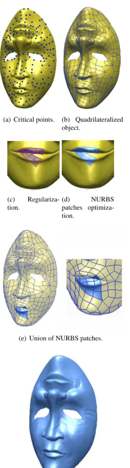
This method to obtain critical points was tested with smooth and irregular arbitrary topology of real objects, re-spectively (See Figure 1(a)). For each object, the critical points obtained for different harmonics configuration are used.
4.1.2. Critical Points Interconnection. Once critical points are obtained and classified, then they should be nected to form the quadrilateral base of the mesh. The con-nection of critical points is started by selecting a “saddle point” and by building two inclined ascending lines and two declined descending lines. Inclined lines are formed as a vertex set ending at a maximum critical point. In addition, a descending line is formed by a vertex path which ends at a minimum critical point. One can then join two paths if both
are ascending or descending.
After calculating every paths, the triangulation of K surface is divided into quadrilateral regions which forms Morse-Smale complex cells [19]. Specifically, every quadrilateral of a triangle falls into a “saddle point” without ever crossing a path. The complete procedure is described in Algorithm 3:
Algorithm 3: Bulding method of MS cells.
Critical points interconnection();
begin
Let T={F,E,V}M triangulation; Initialize Morse-Smale complex, M=0; Initialize the set of cells and paths, P=C=0; S=SaddlePointFinding(T);
S=MultipleSaddlePointsDivission(T); SortByInclination(S);
foreverys∈Sin ascending orderdo CalculeteAscedingPath(P);
end
whileexists intactf ∈Fdo
GrowingRegion(f, p0, p1, p2, p3); CreateMorseCells(C, p0, p1, p2, p3);
end
M = MorseCellsConnection(C);
end
In Figure 1(b), it is observed how resulting quadrilat-eral patches are adequately formed, and they are directly obtained from intrinsic surface properties, adjusting to the objects’ geometry.
4.2. Regularization of the Quadrilateral Border
Curves
Because the surface needs to be fitted using NURBS patches, it is necessary to regularize the quadrilateral curves obtained from the mesh. The curves are regularized and fit-ted by b-splines using the following Algorithm 4.
One of the quadrilateral border is selected from the mesh, and later a border is selected from each quadrilateral border and its opposite. The initially selected border is random. The opposite order is searched as one which does not con-tain the vertices of the first one. If the first selected border has vertices A and B, it is required that the opposite border does not contain vertices A and B, but the remaining, B and C.
Later, B-splines are fitted on selected borders with a λ density, to guarantee the same points for both borders are chosen, regardless of the distance between them. In general, a B-spline does not interpolate every control point; there-fore, they approximate curves which permit a local manip-ulation of the curve, and they require fewer calcmanip-ulations for coefficient determination.
Algorithm 4: Quadrilateral mesh regularization method..
Regularization();
begin
1. Quadrilateral selection;
2. Selection of a border of the selected quadrilateral and its opposite;
3. Regularization using B-splines with lambda density;
4. Regularized points match by means of geodetics FMM;
4.1 Smoothing of geodetic with B-splines; 5. Points generating for every B-spline line with lambda density;
end
Having these points at selected borders, it is required to match them. This is done with FMM (Fast Marching Method). This algorithm is used to define a distance func-tion from an origin point to the remainder or surface with a computational complexity ofO(n×logn). This method
in-tegrates a differential equation to obtain the geodetic short-est path by traversing the triangle vertices.
At the end of the regularization process, B-splines are fitted on geodetic curves and densityλpoints are generated at every curve which unite the border points of quadrilateral borders, to finally obtain the grid which is used to fit the NURBS surface.
4.3. Fitting of Optimized NURBS Patches Using an
Evolutionary Algorithm
This section presents a method based on an evolutionary strategy (ES), to determine the weights of control points of a NURBS surface, without modifying the location of sampled points of the original surface. The main goal is to reduce the error between the NURBS surfaces and the data points inside the quadrilateral regions. In addition, the algorithm make sure that theC1continuity condition is preserved for all optimized NURBS patches. The proposed algorithm is described in Algorithm 5.
4.3.1. Optimization of NURBS Parameters. A NURBS surface is completely determined by its control pointsPi,j.
The main difficulty in fitting NURBS surface locally is in finding an adequate parametrization for the NURBS and the ability to automatically choose the number of control points and their positions. The NURBS’s weight function wi,j
determine the local influence degree of a point in surface topology. Generally, weights of control points for a NURBS surface are assigned in an homogeneous way and are set equal to 1, reducing NURBS to simple B-spline surface. The determination of NURBS control points and weights
Algorithm 5: Optimization and continuity method of NURBS patches method.
Adjustment by optimized NURBS patches();
begin
1. Optimization of the NURBS patches; 1.1. Multiple ES usage with deterministic replacement by inclusion;
1.2. Application of ES to control weights of NURBS;
2. Union of NURBS patches with continuityC1; 2.1. Check continuity between axis; 2.2. Check continuity at vertices;
end
for arbitrarily curved surfaces adjustment is a complex non-linear problem.
The minimization problem can be expressed by:
δ= np X l=1 Zl− n X i=0 m X j=0
Ni,p(u)Nj,q(v)wi,jPi,j
n X i=0 m X j=0 Ni,p(u)Nj,q(v)wi,j 2 (4)
whereNi,p(u)andNj,q(v)are B-spline basis functions ofp
degree andqin the parametrical directionsuandv respec-tively,wi,j are the weights,Pi,j the control points,andnp
the number of control points. If the number of knots and their positions are fixed, same as the weights set and only the control points {{Pi,j}ni=1}mj=1∈R
, they are consid-ered during minimization of Equation 4, then we have a simpler linear mean square problem. If knots or the weights are considered unknown it will be necessary to solve a non-linear problem. In many applications, the optimal position of knots is not necessary. Hence, the knots location problem is solved by using a heuristic.
The optimization process is formally described as fol-lows: LetPt = {p1,p2, . . . ,pn}a points-set inR3
sam-pled from the surface of a physical object, our problem con-sists ofE(s) = n1 n P i=1 d2(p i, Si)< δ, whered(pi, Si)
rep-resents the Euclidian distance between a point of the setPt
of sampled points of the original surfaceS, and a point on the approximated surface S0. To get the configuration of surface S0,
E is minimized to a tolerance lower than the givenδ. Minimization is performed using an evolution strat-egy(µ+λ)defined as follows:
• Representation Criteria: Representation is per-formed using of pairs of real vectors.
of individuals is performed making outlier individuals ignored.
• Genetic Operators:
– Individual:The initial valueswi, δiof ALELOS
of every individual are uniformly distributed in interval [0.5, 1.5]. This range is chosen because it is where the initial values of ALELOS of indi-viduals are given, which correspond to weights of control points and therefore should not initially set to zero.
– Mutation: Individuals mutation will not be cor-related withn σ0
s(mutation steps) as established in individual configuration, and it is performed as indicated in the following equations:
σi0 = σie(c0.N(0,1)+ci.Ni(0,1)) (5)
x0i = xi+σ
0
i.Ni(0,1) (6)
where N(0,1)is a normal distribution with
ex-pected value 0 and variance1, c0, ci are
con-stants which control the size of the mutation step. This refers to the change in mutation step σ. Once the mutation step has been updated, the mu-tation of ALELOS of individuals is generatedwi.
• Selection Criteria: The best individuals in each gen-eration are selected according to the result of the fitness function.
• Replacement criteria: In ES, the replacement
crite-ria is always deterministic, which means that µor λ best members are chosen. In this case, the replacement by inclusion was used, in which theµdescendants are joined with theλbest members and are taken for the new population.
• Recombination operator: Two types of recombina-tion are applied whether object variableswior strategy
parametersσiare being recombined. For object
vari-ables, an intermediate global recombination is used: b0i= 1 ρ ρ X k=1 bk,i (7)
where b0i is the new value of ALELOi, andρis the number of individuals within the population.
For strategy parameters, an intermediate local recom-bination is used:
b0i=uibk1,i+ (1−ui)bk2,i (8)
whereb0iis the new value of the ALELOi, anduiis a
real number which is distributed uniformly within the interval[0,1].
4.3.2. NURBS Patches Continuity. Continuity in regular cases (4patches joined at one of the vertex) is a solved
prob-lem [12]. However, in neighborhoods where the neighbors’ number is different from 4 (v > 3 → v 6= 4),
continu-ity must be adjusted to guarantee a soft transition of the implicit surface function between patches of the partition. Although diverse continuity schemes between parametric functions exist, two of these approaches have been empha-sized and they have become an industry standard. Continu-ityC0shows that a vertex continuity between two neighbor-ing patches must exist. This kind of continuity only guaran-tees that spaces or holes at the assembling limit between two parametric surfaces does not exists.C1shows that
continu-ity in normals between two neighboring patches must exist. This kind of continuity guarantees a soft transition between patches, offering a correct graphical representation.
In this paper, C1 continuity between NURBS patches
is guaranteed, using Peters continuity model [21] which guarantees continuity of normals between bi-cubical spline functions. Peters proposes a regular and general model of bi-cubical NURBS functions with regular nodes vec-tors and the same number of control points at both of the parametric directions. In our algorithm, Peter’s model was adapted by choosing generalizing NURBS functions, with the same control points number at both of the parametric directions, bi-cubic basis functions and regular expansions in their node vectors.
Continuity Along the Quadrilateral Boundaries: To guaranteeC1continuity between the boundaries of
neigh-boring patches, extreme control points which affect the con-tinuity between patches must be found. Due to data order-ing within the proposed parametrization schema, two adja-cent patches will have the same number of control points at the common axis, regardless of their disposition. To ad-just continuity between axes, control points are calculated on the analyzed boundary, to make it co-lineal with neigh-boring control points on adjacent patches.
Equation 9 illustrates the new position for a control point at givenPejeaxis, wherePAvecis the neighbor point toPeje
at patchB. The new control pointPejeis the medium point
between the two adjacent control pointsPAvecyPBvecwhich guarantees that control points on the axis and their adjacent neighbors at each patch is co-linear.
Peje=
Pvec A +PBvec
2 (9)
Continuity at Quadrilateral Vertices: Continuity at vertices of quadrilateral regions is guaranteed by making sure that every adjacent control points at each vertices is co-planar.
Under the continuity criteria proposed by Peters, conti-nuity at quadrilateral vertices are generalized, that is to say, the adjustment process is the same regardless of the num-ber of patches which can be found at a given vertex. We haveπTP = 0, whereπis a given plane andP is a point
on the plane. If the system of equations is over-determined with more than four points, the equation which best adjusts a given point-set can be found.
Equation 10 represent the over-determined system where P = [P1, P2, . . . , Pn]T withn≥ 4are control points at
the vertices. The equation is solved using Singular Values DecompositionSV D, with the last column of matrixPthe equation of the plane which is adjusted to points-setP in the quadratic mean square error sense. [15].
P1 x Py1 Pz1 1 Px2 Py2 Pz2 1 ... ... ... 1 Pn x Pyn Pzn 1 πx πy πz πz = 0 (10)
Continuity is adjusted by projecting control points P onto the plane given by Equation 10:
π=n1(x−xo) +n2(y−yo) +n3(z−zo) (11)
where N = [n1, n2, n3] is the plane’s normal andP0 =
[x0, y0, z0]is a point on the plane. The projection PI =
[xI, yI, zI]of a pointP = [Px, Py, Pz]on the plane is given
by:
xI =Px+n1tI yI =Py+n2tI zI =Pz+n3tI (12)
where t is the parametric value of the straight line which passes through pointPin the direction of the plane’s normal
N.
Using Equation 12, it is possible to project control points on the given plane, which guarantee the continuity of nor-mals at vertices of the quadrilateral partition, ensuring that every adjacent control points are co-planar.
5. Experimental Results
In this section, the results of the methodology of three-dimensional reconstruction of free-form objects proposed in this paper are shown. To validate the functionality of the proposed algorithm for surface fitting by means of NURBS patches, the results for a free-form object (see Figure 1) are presented.
Tests were performed using a 3.0 GHz dual Opteron processor computer, with 1.0 GB RAM, running Microsoft Windows XP operating system. The methods were imple-mented using C++ and MATLAB. The data used were ob-tained with Kreon range scanners, available at the Advanced Man-Machine Laboratory – Department of Computing Sci-ence, University of Alberta, Canada.
The partial results obtained at each one of the interme-diate stages of the proposed algorithms in this paper are shown in Figure 1. This object called Mask is composed of 18 range images, corresponding to 84068 points. The fi-nal model is composed of 105 optimized NURBS surfaces patches with an adjustment error of1.02×10−3(See
Fig-ure 1(f)). The reconstruction of the object took an average time of 32 minutes.
6. Conclusion
The methodology proposed in this thesis for the automa-tion of reverse engineering of free-form three-dimensional objects has a wide application domain, allowing adjustment of surfaces regardless of topological complexity of the orig-inal objects.
A novel method for fitting triangular mesh using opti-mized NURBS patches has been proposed. This method is topologically robust and guarantees that the complex base be always quadrilateral creating a network of surfaces which is compatible with most commercial CAD systems.
In the proposed algorithm, the NURBS patches are op-timized using multiple evolutionary strategies to estimate the optimal NURBS parameters. The resulting NURBS are then joined, guaranteingC1continuity. The formulation of C1 continuity presented in this paper can be generalized, because it can be used to approximate regular and irregular neighborhoods which present model processes regardless of partitioning and parametrization.
References
[1] Amenta N., Bern M., and Kamvysselis M. A new
voronoi-based surface reconstruction algorithm. Proc. 25th
Inter-national Conference on Computer Graphics and Interactive Techniques, pages 415–421, July 1998.
[2] Amenta N., Choi S., Dey K., and Leekha N. A simple
al-gorithm for homeomorphic surface reconstruction. Proc.
16th Annual ACM Symposium on Computational Geometry, pages 213–222, June 2000.
[3] Arge A., Daehlen M., and Tveito A. Approximation of scat-tered data using smooth grid functions. Technical Report STF33 A94003, SINTEF, 1994.
[4] Baxter B.The interpolation theory of radial basis functions.
PhD thesis, Trinity College, University of Cambridge, 1992. [5] Bernardini F., Mittleman J., Rushmeier H., Silva C., and Taubin G. The ball-pivoting algorithm for surface
recon-struction. IEEE Transactions on Visualization and
Com-puter Graphics, 5(4):349–359, /1999.
[6] Boissonnat J. and Cazals F. Smooth surface reconstruc-tion via natural neighbor interpolareconstruc-tion of distance funcreconstruc-tions. Computational Geometry, 22(1-3):185–203, 2002.
(a) Critical points. (b) Quadrilateralized object.
(c)
Regulariza-tion. (d)patches optimiza-NURBS tion.
(e) Union of NURBS patches.
(f) Fitted surface by the opti-mized NURBS patches.
Figure 1. Reconstruction of a complex curve sur-face using a network of NURBS patches.
[7] Boyer E. and Petitjean S. Curve and surface reconstruction from regular and non-regular point sets. pages 659–665, 2000.
[8] Carr J., Beatson R., Cherrie J., Mitchell T., Fright W., Mc-Callum B., and Evans T. Reconstruction and representation of 3d objects with radial basis functions. In Eugene Fiume,
editor,SIGGRAPH 2001, Computer Graphics Proceedings,
pages 67–76. ACM Press / ACM SIGGRAPH, 2001. [9] Cohen-Steiner D. and Da F. A greedy surface reconstruction
algorithm.Visual Computer, 3:113–146, 1994.
[10] Dey T. and Goswami S. Provable surface reconstruction
from noisy samples.Computational Geometry: Theory and
Application, 35(1-2):124–141, 2006.
[11] Dong S., Bremer P., Garland M., Pascucci V., and Hart J.
Quadrangulating a mesh using laplacian eigenvectors.
Tech-nical Report UIUCDCS-R-2005-2583, 2005.
[12] Eck M. and Hoppe H. Automatic reconstruction of b-spline
surface of arbitrary topological type. ACM-0-89791-747-4,
8, 1996.
[13] Edelsbrunner H. and Mucke E. Three-dimensional alpha
shapes.ACM Transactions on Graphics, 13(1):43–72, 1994.
[14] Gopi M., Krishnan S., and Silva C. Surface reconstruction based on lower dimensional localized delaunay triangula-tion. volume 19, pages C467–C478, 2000.
[15] Hartley R. and Zisserman A. Multiple view geometry in
computer vision. Cambridge University, second edition,
2003.
[16] Hoppe H. Surface reconstruction from unorganized points.
PhD thesis, Washington University, 1994.
[17] Levin D. Mesh-independent surface interpolation. Technical report, Tel Aviv 69978, Israel, 1999.
[18] Loop C. Smooth spline surfaces over irregular meshes.
Ap-ple Computer Inc., 1994.
[19] Ni X., Garland M., and Hart J. Fair morse functions for
extracting the topological structure of a surface mesh.ACM
Trans. Graph., 23(3):613–622, 2004.
[20] Ni X., Garland M., and Hart J. Simplification and repair of
polygonal models using volumetric techniques. Proc.
SIG-GRAPH, TOG 23,3,613-622, 2004.
[21] Peters J. Constructingc1surfaces of arbitrary topology
us-ing bicuadric and bicubic splines. Designing Fair Curves
and Surfaces, 277-293, 1994.
[22] Savchenko V., Pasco V., Okunev O., and Kunni T. Function representation of solids reconstructed form scattered surface
points and contours.Computer Graphics Forum, 14, 1995.
[23] Turk G. and O’Brien J. Shape transformation using
vari-ational implicit functions. Computer Graphics, 33(Annual
Conference Series):335–342, 1999.
[24] Weber G., Scheuermann G., Hagen H., and Hamann B. Ex-ploring scalar fields using critical isovalues. 2002.