quantity flexibility contracts and spot
procurement in a supply chain
Xavier Brusset
∗ †May, 2nd, 2005
Abstract
When, in a supply chain, a supplier and a buyer have the choice of transac-tion form to do business, the equilibrium transactransac-tion form which emerges is much more constrained than previously envisaged in literature. In this paper, two forms of long-term supply contracts and procurement in the spot market are compared. A capacity constrained service provider and a buyer of such service choose among three different transaction forms: spot procurement, minimum purchase commitment and quantity flexibility contracts. The ulti-mate demand the buyer has to satisfy and the spot market price of the input she has to purchase from the supplier are exogenous stochastic processes. Complete analytical results and a numerical example are presented. This paper builds upon recent supply chain contract literature by trying to join in one setting problems which up till now were considered in isolation.
Keywords: contract, supply chain, spot market, procurement strategies, mini-mum purchase commitment, quantity flexibility
∗IAG, Université Catholique de Louvain, Louvain la Neuve, Belgium – E-mail: [email protected]
†I wish to thank particularly my thesis supervisor, Prof. Per Agrell, for his encouragements and inspiring comments and Prof. Yves Pochet for his help in mathematical matters.
1
Introduction
Usually, in most literature about supply chain management literature, the choice of transaction form is exogenously given and hence the equilibrium is probably non-efficient as compared to the one achieved in an endogenously defined transaction form adopted at equilibrium by the two partners. Some results of ongoing research are presented here which focus on the relationship between, on one side, a firm, which will be called « the buyer » (she), who has to satisfy demand emanating from her own downstream customers; and on the other side a provider (he) who sells a service indispensable to the accomplishment of the buyer’s activity towards those customers.
This service is bought through long term contracts and any additional need is satisfied through some form of backup market "on the day" at "spot" prices.
The question addressed is how the buyer and provider will agree on a type of transaction to adopt and, if a contract is retained, what will be the contract parame-ters. Information is asymmetric: the provider does not know the characteristics of the demand addressed to the buyer, whereas both know of the distribution function of the spot market price.
Three types of transactions are compared and the resulting optimal parameters derived so that Nash equilibria can emerge. The first is the procurement using the spot market. The second uses a contract based on minimum purchase com-mitment and the third is a quantity flexibility clause contract. In the next section, we review relevant literature, in §3, we describe a model; in §4 we give classical equilibria when the choice of transaction form is exogenously defined, then in §5 we compare each type of transaction and define the best form given characteristics of the distributions of spot price and demand. In §6 we give a numerical example before concluding.
2
Literature review
Wuet al. (2002) study the contracting arrangements in energy sector between a producer and several buyers. They derive the optimal contract parameters when price of the input is a deterministic function of the received demand. Both buyers and providers can take recourse in the spot market for "on the day" transactions to satisfy their needs. Their solution involves deriving demand from spot price or vice versa. Kleindorfer & Wu (2003) and Spinler & Huchzermeier (2005) provide variations on the preceding where the use of options in the context of B2B
markets is studied. The present paper calls upon the same modeling framework along a three-period time line but with stochastic price and demand which may be dependent. The focus here is on a "must-produce-must-exercise" option based contract (called "forward contract" in Kleindorfer & Wu (2003)). Chen (2001), in a one buyer-multiple seller model, derives an efficient procurement strategy through a comparison of two auction mechanisms. In the first, the provider offers a quantity given a scale of price-quantities from the buyer and in the second, the supplier offers a price for a quantity taken from a scale of quantities provided by the buyer. All suppliers are symmetric and the least cost supplier wins.
In all the above, the buyer must reduce unit procurement cost for a given de-mand risk. In other words, she must offload the risk onto the provider. Some measure of flexibility in capacity has to be introduced. InMoinzadeh & Nahmias
(2000) that same general problem is treated: Q, the minimum commitment per pe-riod is given and there are both fixed and proportional penalties for adjustments, over an infinite horizon. The authors contend, but do not formally prove, that a type of order-up-to policy(s, S)is optimal. In that model, the fixed delivery con-tract with penalties serves as a risk sharing mechanism. In our model, because the demand, when realized, directly results in a buying requirement, there can be no time-flexibility arrangements as those described in the literature (Li & Kouvelis,
1999). In our approach, production capacities are not freely substitutable, ruling out "overbooking" (Karaesmen & van Ryzin,2002).
Seifert et al. (2004) studies a model of spot markets for commodities that can be stocked and are subject to obsolescence and quick price fluctuations. We inspire ourselves from this paper to model the procurement strategy for the spot market. The most significant result is that profit improvements can be achieved if a moderate fraction of the commodity demand (in our case this is our input demand) is procured via the spot market. In this paper, both the demand addressed to the buyer and the price of the commodity can vary. However, commodities can be salvaged which is not part of our model.
Lariviere (1999) models several types of contracts in a newsvendor setting with demand as a stochastic process. The purpose is to achieve an efficiency level as close as possible to the efficiency of a centralized organization. The players do not engage in negotiation of the contracts or parameters.
Corbett & Tang(1999) study three common types of contracts, each a special case of the next: the basic wholesale-pricing scheme, a two-part linear scheme with fixed wholesale price and side payment, and a two-part nonlinear scheme with wholesale price and side payment depending on quantity purchased. The best contract is defined given information asymmetry scenarios but all models
share the same deterministic demand assumption.
Tsayet al. (1999) review and classify several types of contracts, however all involve goods that can be stocked and backlogged. Quantity flexibility clauses and minimum purchase commitments are established as coordinating mechanisms in a supply chain.
Cachon & Lariviere(2001) draws attention on the information imbalance preva-lent in most supply chains which has special consequences when the supplier is hamstrung by tight capacity and varying contract compliance (full or voluntary on the provider’s part). That paper studies contracts that allow the supply chain to align incentives, correcting these imbalances. In their setting, the buyer solicits the provider for too much capacity so as to be able to meet more than the aver-age expected demand. The provider must contrive a contract which enables the buyer to credibly signal the necessary capacity. The results proven inCachon & Lariviere (2001) are: the supply chain is better coordinated under assumption of asymmetric information when both players set up a firm commitment for capacity for which the buyer promises to pay a lump sum upon realization of demand.
Bassok & Anupindi(1997), later revisited inAnupindi & Bassok(1998) and elaborately discussed inTsay & Lovejoy(1999),Tsay(1999), describes in detail the contract model which inspires us here: the total minimum quantity commit-ment where a buyer guarantees that his cumulative orders across all periods in the planning horizon will exceed a specified minimum quantity. In this model, a single product is studied; excess product can be stored and unsatisfied demand can be backlogged. No secondary source for the product is included. The solu-tion is a bootstrap of a stochastic dynamic program. We have added to the basic description of this contract in this paper an incentive that ensures coordination in the supply chain.
To explain the choice of the three forms of contracts used here, the reader can refer to the arguments developed inBarnes-Schusteret al. (2002) which give examples of use of similar contracts in industry and states "clearly, channel co-ordination is always achieved when the buyer is able to internalize the costs of the supplier". The provider in our setting specifically suffers from constrained capacity and a fixed plus variable cost for operating this capacity. Moreover, be-cause the demand, when realized, directly results in a product requirement, there can be no time-flexibility arrangements1 as those described in the literatureLi & Kouvelis(1999). Plambeck & Taylor(2003) andPlambeck & Taylor(2005) give 1The carrier can tell his customer: "Your order is too big for our available capacity today, we can still provide you next-day service at a discount."
an extensive discussion of a game of repeated informal trade agreements where both members of the supply chain have to negotiate investment into productive capacity ahead of demand under diverse assumptions of information asymmetry.
3
Description of the model
3.1
General setting with bivariate output demand and input
price
In the present model, both buyer and provider are price takers. Contrary to the energy markets described inWuet al. (2002), service markets are not well orga-nized (for example, the freight matching exchanges never really took off), so we model information as being sparse and costly.
As opposed to most newsvendor settings, the contracted service cannot be backlogged. Further, no storage, holding or shortage costs are incurred. The sup-ply lead time is assumed to be zero. The provider cannot deliver less than the amount ordered by the buyer if he has available capacity to produce this amount: he works under a regime offorced compliance(Cachon,2004), which means that the supplier delivers the amount not to exceed the retailer’s order that maximizes her profit given the terms of the contract; so the possibility of the provider volun-tarily restraining his delivered quantity to the buyer is not contemplated. Further-more, the service that has to be delivered is produced through capacity constrained equipment.
The non-storability aspect of this problem gives rise to the so-called two-goods problem: contracted, available capacity at a given price and additional capacity at another price (different conditions). This setting is also related to the problem of the producer producing two goods in a joint production process and choosing between technologies with different costs and cost structures. This could typically be the case of the provider sub-contracting capacity from third parties to offer it to the buyer in a bid to increase service quality. The key issue we study here is how spot pricing and bilateral contracting are or should be linked. From the provider’s perspective, pre-committing capacity at a fixed price may exclude more profitable opportunities through the spot market on the day. The same is true for the buyer. The key trade-off in determining how such contracts should be priced and how much capacity should be committed to them by providers and buyers are the relative costs and risks of sourcing from the contract versus the spot market.
exoge-nous demandQthat has a continuous at least twice differentiable unimodal distri-butionFq(Q)on non-negative reals with densityfq(Q), meanµqand varianceσq2.
The spot market price of service capacityP is also assumed to be an independent, identically distributed exogenous variable following a continuous, twice differ-entiable, unimodal distributionFp(P)on non-negative reals with densityfp(P),
mean µp and variance σ2p. The spot market price is assumed to be uninfluenced
by either the provider or the buyer. We are facing a two-stage stochastic decision process. The buyer’s residual demand not covered by the long-term contract is re-solved by buying additional capacity from the spot market at the day’s spot price. The spot price may vary but is assumed to stay above the variable costv of offer-ing the service as neither the provider nor any other provider of similar service in the market would sell under this common variable cost. In the same way, let us call F the continuous, twice-differentiable joint unimodal distribution and f the joint density function ofP andQwith meanµand varianceσ2.
The mean and standard deviation of demand is assumed to be private knowl-edge of the buyer. The information about the spot market price, mean, variance and distribution is assumed to be common knowledge.
Along the time-line, events happen in the following order. First, the buyer knows of the future demand she has to satisfy. She turns to the provider and negotiates a contract for capacity. Some parameters of the contract are agreed upon. Then, at each period (say every day), demand and spot price are revealed and buyer calls upon sufficient quantity of service from the provider to meet the demand addressed to her. If the committed capacity by contract is insufficient, within the same period, she turns to the spot market and buys additional service at the going spot price. Finally, service and payout are performed within the same period.
3.2
Types of contracts
Two types of contract are used and the utility they provide is compared with the one resulting from the alternative of procuring all service capacity from the spot market. One key difference with other models using contracts and spot markets is that the process of buying capacity from the spot market is assumed to entail a higher cost than the one attributed with contract buying. This is due to the fact that information gathering, service quality and price discovery all have a cost sig-nificantly higher than the transaction cost involved in buying from the contracted provider. This helps to steer away from trivial situations where the buyer might be always better off by buying capacity from the spot market since by essence, this is
the market where overall excess capacity by all providers is offered. Under weak regulatory assumptions, it is straightforward to show that the provider’s optimal strategy is to bid his unit marginal production cost, meaning the variable cost in our model. By essence, this spot market will be cleared by a spot price close to the marginal cost of operating all available capacity among providers. However, two factors impede the spot price from equating the variable cost. One factor results from tensions due to high demand from buyers (take for instance the case of the wheat harvest having to be carried by truck to silo facilities in countries where the railroad infrastructure is insufficient). The other factor stems from market opacity and information cost that impede the perfect clearing of all bids and offers at the most efficient price.
The objective functions for the buyer and provider under three settings are described: spot procurement, a minimum purchase commitment contract and a contract with single price but with quantity flexibility clause. In each case, the objective functions when both demand and spot price vary are spelt out. We then compare each contract to spot buying in order to present insights on the alternative open to the buyerbeforecontracting.
3.3
spot procurement
The buyer’s objective function is a cost function which can be modeled as:
V1(Q, P) = U(Q)−P Q−I (1)
whereU is the utility function for the buyer andI (I >0) is the transaction cost differential between spot market and contract mechanisms that affects both buyer and provider. The provider’s objective function is a profit function which can be modeled as
π1(Q, P) =P Q−V Q−C−I (2)
where V is the variable cost for producing quantity Q, C is the fixed cost at-tributed to operating the service capacity. The provider will be considered here to have only one technology at his disposal and hence that his production facil-ity is homogeneous which simplifies fixed cost attribution. Using the properties of the expectation of the product of two random variables and assuming that the utility function is an additive function, the expected values for the buyer can be represented. Superscript p for the provider and superscript b for the buyer are
used.
E1b = E(V1(Q, P))
= U(µq)−Cov(Q, P)−E(Q)E(P)−I
= U(µq)−Cov(Q, P)−µqµp−I. (3)
for the provider:
E1p = E(π1(Q, P))
= Cov(Q, P) +µqµp−V µq−C−I. (4)
Observe that the higher the covariance of spot and demand, the higher the profit to the provider! This, among other reasons, explains why providers’ profits in niche markets are dependent both upon the existence of tight capacity niche-wide (which causes volatility of the spot price for this capacity) and of high demand volatility. In point of fact, lifting the capacity constraint, through new players entering the market or through existing players adding capacity, may be uneco-nomical in the short term because of the high volatility of the marginal revenue.
3.4
Minimum purchase commitment contract
The minimum purchase commitment as studied in Cachon & Lariviere (2001), consists in afixed feerthat the buyer agrees to pay the provider each period pro-portionate to an agreed capacity committed q and a variable feec for each unit effectively bought in the period. The fixed fee is paid whether the buyer uses the capacity or not. As proven in Cachon & Lariviere (2001), it is a coordinating mechanism to ensure that the buyer (who has private information on the demand she will face before the contract is signed) will not over-estimate the service ne-cessity and that she will use it independently from the level of the spot price. This mechanism differs from the one exposed inWuet al. (2002). There, the buyer can still take advantage of the spot market when the spot price is less than the variable part of the two-part tariff in the contract. The contract described is also called a two-part tariff for minimum commitment purchase. In the present model, as op-posed toCachon & Lariviere(2001), the buyer can still complement his realized demand from the provider if this demand exceeds the committed quantity to be bought. As exemplified inSeifertet al. (2004), in the present model this excess demand is paid at the going spot market price. There is no clear cut connection between the contract modeled here and the expected transfer payment of the con-tract in Cachon & Lariviere (2001), but the gist of the mechanism is reflected,
namely a lump sum payment plus a variable rate per item. This is justified by the adaptation of this form of payment to the real cost structure of the provider (fixed cost plus variable cost).
The sequence of operations is the following. At first the buyer knows of future demand she must address. This information is private to her but she signals to the provider about the expected level by asking for capacity equal to the expected demand. Both she and the provider share knowledge as to average and standard deviation of the spot market price. So she negotiates with the provider a contract. Parameters are agreed upon: r, q, c. Then demand and the spot market price are realized. The buyer buys the necessary good from the provider who delivers. Payout occurs.
We can write:
V2(Q, P) = U(Q)−r−max(q, Q)c−(Q−q)+P (5)
where(Q−q)+ denotes that ifQ < qthen(Q−q)+ = 0andQ−qotherwise.
For the provider:
π2(Q, P) = r+max(q, Q)c+ (Q−q)+P −V Q−C. (6) The provider can still sell additional capacity to the buyer at the going spot price of the day if received demand exceeds the minimum capacity committed.
We will consider in the following that the expected utility to the buyer of the demand can be written E(U(Q)). The expected profit to the provider and value to the buyer are functions of q, c, r, contract parameters which become the decision variables of both buyer and provider. We define g(P, Q) = P(Q−q)
and a function ϕ(.). From the definition of the conditional distribution and of conditional expected values,
ϕ(q) = E(g(P, Q)|Q > q) ϕ(q) = Z ∞ v Z ∞ q (x−q)yf(x, y)dxdy. (7) So we get E2b(q, c, r) = E(V2(Q, P)) = E(U(Q))−r−cµq(q)−ϕ(q) (8)
withµq(q)as the expected demand between0andq. For the provider:
E2p(q, c, r) = E(π2(Q, P))
The interesting variable to determine is the optimal quantityq∗, object of the com-mitment. We now see what this optimal capacity is.
3.4.1 Discrete distribution
Without loss of generality, it can be considered that the continuous distribution functions are in fact extensions from discrete functions in the real world.
Theorem 1 (Characterization of the optimal q). If there exist optimal quantities that satisfy both supplier and buyer, then theseq∗must satisfy the following equa-tion:
pq(q∗)(q∗−µq) = pq(q∗+ 1)(q∗+ 1−µq), (10)
wherepqis the marginal discrete probability function of the demand.
See appendixAfor the proof.
We see that solving this equation very much looks like finding the root to a differential equation where the step, which is here set to one, is a quantity h
which tends to zero.
Going back, if we take the discrete distribution to have a step ofh, we still get to the same result. So to achieve a result that is applicable to a continuous density function, we lethtend to zero.
We can formalize it as a functiong
(
g(x) = fq(x)(x−µq), x≥0
g(x) = 0, x <0 (11)
with fq(.)andµq as previously defined. To solve (10), we need but look for the
roots of the differential of the first order:
∂g(q∗)
∂x = 0
fq0(q∗)(q∗−µq) +fq(q∗) = 0 (12)
Lemma Even when both demand and price of a necessary input fluctu-ate, the optimum quantity to be contracted is independent from the price of that input. The optimal quantities satisfy the equation (10) when the distribution of the quantity is discrete and (12) when it is continuous.
3.4.2 Instance using normal and exponential distributions
Different distribution functions yield different results for optimalq∗. The normal distribution ofQyields two roots:
q1∗ =µq−σq q2∗ =µq+σq (13)
The exponential distribution yields just one root:
q∗ = 2µq. (14)
3.5
Quantity flexibility contract
In the same way as described inBassok & Anupindi(1997), we can write the ob-jective and expected obob-jective functions when the contract is for a variable price
mbut the buyer signs for multi period minimum quantity commitment. To ensure coordination, as mentioned in the literature review (Chen, 2004), we include a mechanism which limits the buyer from contracting a too high committed min-imum quantity. This is represented in our model by a penalty θ. This penalty cannot be higher than the expected spot priceµp nor higher than mor the buyer
would not enter into such a contract. Lett be the number of periods over which the committed quantity W has to be purchased; the game has to be repeated t
times.
In the first case, there is a number of periods, lower or equal than t, during whichW has been purchased. The recourse for the buyer is to purchase additional quantities from the supplier or from the spot market at the revealed going spot pricePiin periodiand duringjadditional periods within the totalt. She chooses
to transact with the supplier since these later transactions do not face the added information cost I that characterizes transactions on the spot market since both parties already know each other and the spot price is assumed to be common information to both parties.
In the second case, when the buyer underestimates the demand she receives, she has to pay a penaltyθtimes the quantity shortfall.
The whole discussion of the optimal contract parameters turns around this shortfall. W ≥ t X i=1 Xi, V3(X, P) = t X i=1 U(Xi)−m t X i=1 Xi−θ(W − t X i=1 Xi) π3(X, P) = m t X i=1 Xi+θ(W − t X i=1 Xi)−c t X i=1 Xi−tK
W < t X i=1 Xi, j|j ≤t ∧ t−j−1 X i=1 Xi ≤W ∧ t−j X i=1 Xi > W, V3(X, P) = t X i=1 U(Xi)−mW −( t−j X i=1 Xi−W)Pt−j − t X i=t−j+1 PiXi π3(X, P) = mW + ( t−j X i=1 Xi−W)Pt−j+ t X i=t−j+1 PiXi)−c t X i=1 Xi−tK
Let a functionΨdescribe the evolution of this part of the profit function for both buyer and supplier. It is discussed inBand is defined in (51).
Given that all periods of the game are symmetric in terms of the expected outcome and that each demand outcome is i.i.d. w.r. to the others and the spot prices are also i.i.d. w. r. to the other spot prices, the buyer’s and supplier’s expected profit functions are
E3b(m, W, θ, t) = thU(µq)−mµq i −Ψ(W, θ, t) E3p(m, W, θ, t) = t h mµq−cµq−K i + Ψ(W, θ, t), (15) subject to 0≤θ < m (16) The longer the contract (higher t), the lower the variance of the sum of expected demands, reducing the impact of both penalty and spot prices. At the limit,when
lim
t→∞µY(W, t) = 0,
which effectively means that both supplier and buyer will be indifferent to the level ofθbecause they won’t need it! It is interesting to discuss the behaviour of
ΨwhenW,µq andtare "proportional": for example whenW =tµq.
Given that the players have incurred sunk investments in their relationship, they both aim to increase the length of the contract. The partial differentials in t
of their profit functions must be positive or null:
∂E3b(m, W, θ, t) ∂t =U(µq)−mµq− Ψ(W, θ, t) ∂t ≥0 ∂E3p(m, W, θ, t) ∂t = +mµq+ Ψ(W, θ, t) ∂t −cµq−K ≥0 (17)
These inequations provide us with conditions onm: m≤U(µq) +∂Ψ(W, θ, t)/∂t µq m≥cµq+K +∂Ψ(W, θ, t)/∂t µq (18)
Proposition 1. For the QFC to be chosen by both supplier and buyer, the contract parametersm, W, θ, tmust meet the following conditions
t 0 W| max(W < tµq) θ < m, m ≤U(µq) +∂Ψ(W, θ, t)/∂t µq m ≥cµq+K+∂Ψ(W, θ, t)/∂t µq . (19)
4
Helping buyer and provider to choose a sourcing
strategy
Should the buyer enter into a contract or just choose short term spot market buy-ing? If she chooses the contract, at what parameters so that, to her, the outcome is not worse than sticking with the spot market?
We can now compare the different forms of transactions. Let us start with the comparison of the minimum purchase commitment(MPC) and spot, we then will compare theQuantity Flexibility contract(QFC) with the spot; finally, we compare both contracts.
It must be pointed out here that the restriction on the utility function having to be distributive over the sum can be relaxed since it does not appear again in the following comparisons and it does not change the results which are used here.
4.1
Minimum commitment versus spot
The difference between the expected values to the buyer of the MPC and spot to the buyer is labeled D2−1, it is a function of the contract parameters c, q and r
which become the decision variables for buyer and provider. From (3) and (8) we can write: D2b−1(q, c, r) = E2b(q, c, r)−E1b = Cov(Q, P) +µqµp+I−r−cµq(q)−ϕ(q) D2p−1(q, c, r) = E2p(q, c, r)−E1p = −Cov(Q, P)−µqµp+I+r+cµq(q) +ϕ(q). (20)
We are interested in the sign of this difference so as to decide which procurement strategy is best. Here the interests of provider and buyer go in opposite direction except for the cost of information.
Theorem 2(Conditions for choosing MPC over spot). For both parties to choose the MPC means that the contract parameters must satisfy
Cov(Q, P) +µqµp−r−cµq(q∗)−ϕ(q∗)
≤I
fq0(q∗)(q∗−µq) +fq(q∗) = 0
(21) As can be seen, the higher the covariance of spot price and demand, the higher the contract cost to entering a contract for both parties. This is a rational justifi-cation to the observed practice in the market for transport services. Shippers will more often stick with the spot market when the volatilities observed in the spot price and demand are small compared to the information cost.
If the buyer chose the contract, she would choose the optimal quantityq∗ de-fined in (12); replacing in (20), we derive the necessary conditions onrandc:
Cov(Q, P) +µqµp+I−cµq(q∗)−ϕ(q∗) ≥ r Cov(Q, P) +µqµp−I−cµq(q∗)−ϕ(q∗) ≤ r (22) 1 µq(q∗) h Cov(Q, P) +µqµp+I−r−ϕ(q∗) i ≥ c 1 µq(q∗) h Cov(Q, P) +µqµp−I−r−ϕ(q∗) i ≤ c (23)
These closed segments are the restricted values that{r, c}can take for the contract to be elected. Any value outside of these segments will result in each player choosing a different form of transaction. The segments are proportional to the information cost. The higher this cost, the larger the segment. If the information cost is null, just one value can satisfy choosing the contract over the spot market.
4.2
Quantity flexibility versus spot
We have to find when the buyer is indifferent to signing a quantity flexibility contract or buying from the spot market. Let us call D3−1 the function in terms
oft, W andθof the difference between both expected values overt periods. We are again interested in defining when this function is positive or negative. We distinguish between cases when the contracted committed capacity is less than the expected demands and the case when the contracted commitment is higher or equal to the expected demand.
From (3) and (15), we define
D3b−1(m, W, θ, t) = E3b(m, W, θ, t)−tE1b. Db3−1(m, W, θ, t) =t Cov(Q, P) +µqµp+I −mtµq−Ψ(W, θ, t) (24)
which is dependent onm,tandθ.
For the provider, the expected difference comes from (4) and (15):
Dp3−1(m, W, θ, t) =t
I−Cov(Q, P)−µqµp
+m tµq+ Ψ(W, θ, t); (25)
which, except for the information cost, is the exact opposite from what the buyer is aiming for. In practical terms, for both players to choose the contract means that we need to have both (24) and (25) positive.
The only region when the players will choose the contract over spot market trading is when these expected differences are of identical signs. Becauset > 0, the values ofθwhich satisfy this condition are
1 t −Cov(Q, P)−µqµp+mµq+tΨ(W, θ, t) ≤I. (26)
The other condition which would otherwise lead the buyer to refuse the con-tract (seen when presenting the concon-tract in 3.5), is that θ < m. We enounce the theorem
Theorem 3(Conditions for choosing QFC over spot). For both players to choose the Quantity Flexibility Commitment over the spot market, the following condi-tions have to be met:
I ≥ 1 t −Cov(Q, P)−µqµp+mµq+tΨ(W, θ, t) θ < m t 0 (27)
Any "large" value ontwill push the players to choose the contract over spot market transactions because the overall variance of the sum of demands will be low, reducing the need to have high penalties. The range of values available is once again proportionate to the information cost I. If information about prices and providers was costless, decision variables would have just one equilibrium value for the contract to be selected.
The higher the value oft, the bigger the incentive.
If these conditions are not met, the contract will not be retained; the players will choose to transact their business through the spot market paying the informa-tion cost.
4.3
Deciding between a QFC and a MPC contract
We now try to help the buyer choose between both, given the conditions in spot price and demand she receives. Let us callD3−2the difference between QFC and
MPC in terms of all the decision variables. From (8) and (15) we have
Db3−2(q, c, m, r, t, W, θ) =E3b(m, t, W, θ)−E2b(q, c, r)
=t(r+cµq(q) +ϕ(q))−mtµq−Ψ(W, θ, t) (28)
In the same way, from (9) and (15), we get
Dp3−2(q, c, m, r, t, W, θ) = mtµq + Ψ(W, θ, t) − t(r+cµq(q) +ϕ(q)) (29)
We are interested in the sign of each function. We see that ifD3b−2(q, c, m, r, t, W, θ)>
0, then D3p−2(q, c, m, r, t, W, θ) < 0, which means that if the buyer chooses the MPC, the provider will choose the QFC and vice versa. The only possible equi-librium is for both to choose the same contract which is only feasible when
D3p−2(q, c, m, r, t, W, θ) = D3b−2(q, c, m, r, t, W, θ) = 0.
This means that for both to choose the same contract, both contracts have to offer the same expected profits to each of the players.
follow-ing set of inequations and equations have to be solved mµq+ Ψ(W, θ, t) =r+cµq(q) +ϕ(q) fq0(q)(q−µq) +fq(q) = 0 W < tµq θ < m t0. (30)
Additionally, the following conditions have also to be met for a contract to be chosen as opposed to the spot market: (1), (21) and (26).
We have now proved that these are no trivial values and that they depend on the terms of the bivariate distributions and the cost of information.
Theorem 4 (Conditions for choosing QFC over MPC). For a contract to be re-tained versus the price-only relational form and then for the QFC to be chosen over the MPC, the following conditions have to be met:
mµq+ Ψ(W, θ, t) = r+cµq(q) +ϕ(q) fq0(q)(q−µq) +fq(q) = 0 W < tµq θ < m t0 1 t −Cov(Q, P)−µqµp+mµq+tΨ(W, θ, t) ≤I m≤ 1 µq (U(µq) +∂Ψ(W, θ, t)/∂t) m≥ 1 µq (cµq+K+∂Ψ(W, θ, t)/∂t). (31)
5
Numerical example
To illustrate graphically the results a numerical example is offered. Letf(Q, P)
be a bivariate normal distribution with the following characteristics:
µq = 10, σq = 3, µp = 5, σp = 2, ρ= 0.5,
the other relevant parameters are
As a consequence, we have
Cov(Q, P) = ρσqσp = 3
µqµp = 50 (32)
The information cost is supported in every period and represents in this example a non-negligible cost compared to the average spot market price. This means that using the spot market induces an overall cost to the buyer 40% higher than what the apparent cost is (the spot price). This fact is often unrecognized in organiza-tions where full administrative costs are not well accounted for.
5.1
Parameters coming form the comparison between MPC
and spot
From (10), we have two possible values for q∗: q∗ = µq − σq = 7, q∗ =
µq+σq = 13
5.1.1 Case whenq∗ = 13
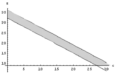
The possible choice between MPC and spot means that the parametersr, c have to fulfill the following condition from (21):
|51.2755−7.68787c−r| ≤2 (33)
which is represented as the grey area in figure 1. As r must be positive (which provider would want to pay the buyer for using his capacity?), we see that c <
(51.2755−2)/7.68787. In the case whenc = (51.2755−2)/7.68787, r = 0, meaning that the fixed fee can be brought to 0 because the variable rate paid by the buyer is sufficient for the provider to want to retain the contract. The width of the range between both lines in gray in figure 1 increases as the information cost. Taking another angle, if demand and spot price are more strongly correlated (ρ→1), the whole range in grey shifts "upwards", meaning that bothrandchave to be increased for the contract to be retained.
5.1.2 Case whenq∗ = 7
In this case, from (21), we get:
Figure 1: ρ= 0.5, q∗ = 13,rmust be in the gray area between both lines
The figure2represents the area thus delimited. When comparing the optimal sets of parameters for both values ofq∗, one sees that the other parameters have to be set higher for the higherq∗ reflecting the higher possibility of the buyer not being able to "fill" the contracted capacity. The previous conclusions aboutρandIalso apply here.
5.2
Parameters coming from the comparison between QFC and
spot
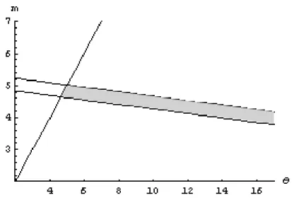
Both buyer and provider have an interest in choosing a "large" t. Let us take
t = 10. SinceW is a function of the number of periods. We chooseW∗ = 100as equal totµq. From (26) we get
(
(10/(10−3))(3 + 50−2−10m)−1.7828≤θ
(10/(10−3))(3 + 50 + 2−10m)−1.7828≥θ (35)
Completed with constraint onm(16), this gives an area forθas shown in grey in figure3.
Figure 2: whenq∗ = 7,candrhave to be higher for a contract to be signed
5.3
Parameters coming from the comparison between QFC and
MPC
We now come to the comparison between both contracts, QFC and MPC. The conditions to be fulfilled are given in (31).
Bear in mind that if a contract is to be chosen, then it also has to dominate the outcome from using the spot market. The solutions for an optimal q∗ = 7are presented, but the same could have been done forq∗ = 13.
5.3.1 Case whenq∗ = 7
The set of conditions becomes
10m+ Ψ(100, θ,10)−r−(µq(7))c−ϕ(7) = 0 |34.323−0.860977c−r| ≤2 |51.8−10m−0.7(1.7828 +θ)| ≤2 c > 0, m >0, r >0, 0< θ < m. (36)
Solving using mathematical software2, we get 16 sets of possible equilibria.
Val-ues of c progressively increase from a low of 0.4324 to a high of 431.227. We 2In this case Mathematicac 5.1 from Wolfram Research
Figure 3: QFC vs spot: possible values for{m, θ}are in grey
give below the conditions for two sets of equilibria for the lowest and the highest values ofc. 0< c≤0.4324 36.319−0.8609c≤r <36.342−0.08428c 1.624 + 0.08044c+ 0.09491r < m≤36.321−0.8609r 401.695< c <431.227 0< r <36.355−0.0843c 1.6243 + 0.08046c+ 0.09346r < m≤36.323−0.861r θ = 24.83 + 1.230c−14.29m+ 1.429r (37)
One set of possible parameters gives
q = 7
c = 0.4324
r = 35.951
5.019< m <5.370⇒m= 5.25
θ = 1.713 (38) The choice ofmis only a matter of power in the relationship between buyer and provider since overall profit of the supply chain is equal.
In conclusion, both MPC and QFC will generate the same value to provider and buyer when:
MPC r = 35.951 q = 7 c= 0.4324 QFC W = 10, t = 10 m = 5.25 θ = 1.713. (39)
Both contracts have higher value than the spot market in the given conditions of demand and spot price distributions.
6
Conclusion
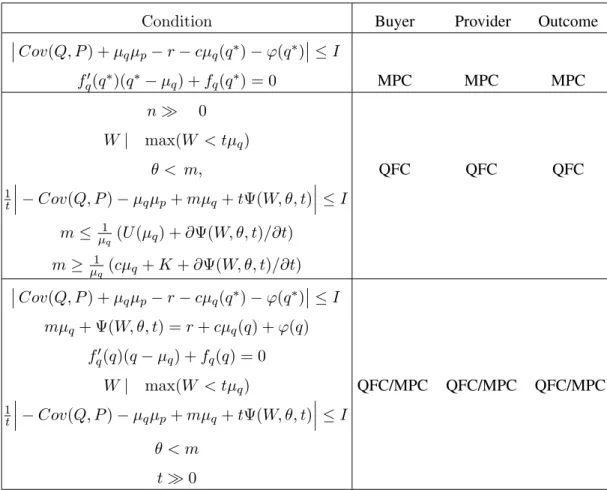
The results established are resumed in table 1 on page 31. Contrarily to con-clusions expressed in the literature which commonly center on just one form of contract or on deterministic demand or input price, the outcome of achoiceof con-tracts leads to very different equilibria altogether. We have formally established how, in an environment of uncertain input prices and uncertain demand and when information is at a premium and asymmetric, the decisions to enter into contracts are taken.
The utility function of the buyer has no influence on the choice she makes as to the transaction form she ultimately chooses: she can be risk averse or risk neutral and still come to the same contractual engagement.
This paper has also established that the contract parameters in a minimum purchase contract, where both input price and demand can vary, are not related to the variance of the price of the necessary input but solely on demand distribution characteristics.
In the process, clear motivations for both provider and buyer to set up formal contractual engagements have been presented.
It is hoped that the material developed here will help to focus future research into the exploration and discussion of alternative supply chain transaction settings in which provider and buyer can interact.
References
ANUPINDI, R., & BASSOK, Y. 1998. Supply contracts with quantity
-SHAN, R., & MAGAZINE, M. (eds), Quantitative models for Supply Chain Management. Dordrecht, Holland: Kluwer Academic.
BARNES-SCHUSTER, DAWN, BASSOK, YEHUDA, & ANUPINDI, RAVI. 2002. Coordination and flexibility in supply contracts with options.Manufacturing & Service Operations Management,4(3), 171–207.
BASSOK, YEHUDA, & ANUPINDI, RAVI. 1997. Analysis of supply contracts with total minimum commitment. IIE Transactions,29(5), 373–381.
CACHON, GERARD. 2004. Supply Chain Coordination with Contracts. Chap. 6, pages 229–340 of: DE KOK, TON, & GRAVES, STEPHEN (eds), Handbooks in Operations Research and Management Science: Supply Chain Management, vol. 11. Elsevier.
CACHON, GERARD, & LARIVIERE, MARTIN. 2001. Contracting to assure sup-ply: how to share demand forecasts in a supply chain. Management Science,
47(5), 629–646.
CHEN, FANGRUO. 2001. Auctioning Supply Contracts. http://www2.gsb.columbia.edu/divisions/dro/working_papers/2001/DRO-2001-04.pdf.
CHEN, FANGRUO. 2004. Information Sharing and Supply Chain Coordination.
Chap. 7, pages 341–421 of: DE KOK, TON, & GRAVES, STEPHEN (eds),
Handbooks in Operations Research and Management Science: Supply chain Management, vol. 11. Elsevier.
CORBETT, CHARLES, & TANG, CHRISTOPHER. 1999. Designing supply
con-tracts: contract type and information asymmetry. Chap. 9, pages 234–267 of: TAYUR, SRIDHAR, GANESHAN, RAM, & MAGAZINE, MICHAEL (eds),
Quantitative models for Supply Chain Management. Dordrecht, Holland: Kluwer Academic.
KARAESMEN, I., & VAN RYZIN, G. 2002. Overbooking with Substitutable In-ventory Classes. Working paper, Columbia University, USA.
KLEINDORFER, PAUL R., & WU, D.J. 2003. Integrating long- and short-term contracting via business-to-business exchanges for capital-intensive industries.
LARIVIERE, MARTIN. 1999. Supply Chain contracting and stochastic demand.
Chap. 8, pages 234–267 of: TAYUR, SRIDHAR, GANESHAN, RAM, & MAG -AZINE, MICHAEL (eds), Quantitative models for Supply Chain Management. Dordrecht, Holland: Kluwer Academic.
LI, CHUNG-LUN, & KOUVELIS, PANOS. 1999. Flexible and risk sharing supply contracts under price uncertainty. Management Science,45(10), 1378–1398. MOINZADEH, KAMRAN, & NAHMIAS, STEVEN. 2000. Adjustment strategies
for a fixed delivery contract. Operations Research,48(3), 408–423.
PLAMBECK, ERICA L., & TAYLOR, TERRY A. 2003 (June). Supply chain rela-tionships and contracts: the impact of repeated interaction on capacity invest-ment and procureinvest-ment. Research Paper nr 1813, Stanford Graduate School of Business.
PLAMBECK, ERICAL., & TAYLOR, TERRYA. 2005. Sell the Plant? The Impact of Contract Manufacturing on Innovation, Capacity, and Profitability. Manage-ment Science,51(1), 133–150.
SEIFERT, RALF, THONEMANN, ULRICH, & HAUSMAN, WARREN. 2004. Opti-mal Procurement strategies for online spot markets. European Journal of Op-erational Research,152(3), 781–799.
SPINLER, STEFAN, & HUCHZERMEIER, ARND. 2005. The valuation of options
on capacity with cost and demand uncertainty. European Journal of Opera-tional Research,NA(NA). available on-line.
TSAY, ANDY. 1999. Quantity Flexibility Contract and Supplier-Customer Incen-tives. Management Science,45(10), 1339–1358.
TSAY, ANDY, & LOVEJOY, W. 1999. Quantity flexibility contracts and supply chain performance. Management Science,1(2), 89–111.
TSAY, ANDY, NAHMIAS, STEVEN, & AGRAWAL, NARENDRA. 1999. Modeling supply chain contracts: A review. Chap. 10, pages 299–336 of: TAYUR, S., GANESHAN, R., & MAGAZINE, M. (eds), Quantitative Models for Supply
Chain Management. Dordrecht, Holland: Kluwer Academic.
WU, D.J., KLEINDORFER, PAUL R., & ZHANG, JIN E. 2002. Optimal
bid-ding and contracting strategies for capital-intensive goods. European Journal of Operational Research,137(3), 657–676.
A
Defining the optimal commitment
Proof. Proof of Theorem1in3.4.1on page10
From (8) the expected value to the buyer is written:
E2b(q, c, r) = E(U(Q))−r−c q X x=1 (q−µq)pq(x)−cµq− ∞ X y=v ∞ X x=q y(x−q)p(x, y), (40) whereas from (9) the expected profit to the provider becomes
E2p(q, c, r) = r+c q X x=1 (q−µq)pq(x) +cµq+ ∞ X y=v ∞ X x=q y(x−q)p(x, y)−V µq−C. (41) What is the optimum quantityqthat the buyer has to contract? If this optimumq∗
exists, and since the buyer wants tomaximizeher utility, it must satisfy:
E2b(q∗−1, c, r)≤E2b(q∗, c, r)≥E2b(q∗+ 1, c, r). (42) The first inequality yields:
E2b(q∗−1, c, r)−E2b(q∗, c, r)≤0 ⇒ −c q∗−1 X x=1 pq(x)(q∗−1−µq)− ∞ X y=v ∞ X x=q∗−1 y(x−q∗+ 1)p(x, y) +c q∗ X x=1 pq(x)(q∗−µq) + ∞ X y=v ∞ X x=q∗ y(x−q∗)p(x, y) ≤0.
When solving, it becomes
c q∗−1 X x=1 pq(x) +cpq(q∗)(q∗−µq) + ∞ X y=v ∞ X x=q∗ y(−1)p(x, y)− ∞ X y=v y(q∗−1−q∗+ 1)p(q∗−1, y) ≤ 0 c 1− ∞ X x=q∗ pq(x) +cpq(q∗)(q∗−µq)− ∞ X y=v ∞ X x=q∗ yp(x, y) ≤ 0;
as the partial probability function can be written in terms of the total probability function, we get c 1− ∞ X y=v ∞ X x=q∗ p(x, y) +cpq(q∗)(q∗−µq)− ∞ X y=v ∞ X x=q∗ yp(x, y) ≤ 0 c pq(q∗)(q∗−µq) + 1 − ∞ X y=v ∞ X x=q∗ (y+c)p(x, y) ≤ 0.(43)
We now study the other inequality:
E2b(q∗+ 1, c, r)−E2b(q∗, c, r)≤0 ⇒ −c q∗+1 X x=1 pq(x)(q∗+ 1−µq)− ∞ X y=v ∞ X x=q∗+1 y(x−q∗−1)p(x, y) +c q∗ X x=1 pq(x)(q∗−µq) + ∞ X y=v ∞ X x=q∗ y(x−q∗)p(x, y) ≤0. As before: −c q∗ X x=1 pq(x)−cpq(q∗+ 1)(q∗+ 1−µq) + ∞ X y=v ∞ X x=q∗ yp(x, y) ≤ 0 −c 1− ∞ X x=q∗+1 pq(x)) −c pq(q∗+ 1)(q∗+ 1−µq) + ∞ X y=v ∞ X x=q∗+1 yp(x, y) ≤ 0 c ∞ X y=v ∞ X x=q∗+1 p(x, y) −c pq(q∗+ 1)(q∗+ 1−µq) + 1 + ∞ X y=v ∞ X x=q∗+1 yp(x, y) ≤ 0 −c pq(q∗+ 1)(q∗+ 1−µq) + 1 + ∞ X y=v ∞ X x=q∗+1 (y+c)p(x, y) ≤ 0. (44)
(44): c(pq(q∗)(q∗−µq) + 1) ≤ ∞ X y=v ∞ X x=q∗ (y+c)p(x, y) ∞ X y=v ∞ X x=q∗+1 (y+c)p(x, y) ≤ c(pq(q∗+ 1)(q∗+ 1−µq) + 1). (45)
Again, without loss of generality, we can safely consider that the “step” in the increase of the discrete probability functionpqcan be narrowed to anhstep, which
means that, reasoning at the limit
lim h→0 ∞ X y=v ∞ X x=q∗+h (y+c)p(x, y) = ∞ X y=v ∞ X x=q∗ (y+c)p(x, y)
Applying this result to (45), we can join both inequalities and since c > 0 by construction, this leads us to an inequality independent from the spot priceP:
pq(q∗)(q∗−µq)≤pq(q∗+ 1)(q∗+ 1−µq). (46)
To resume, if this inequality is satisfied, thenq∗ exists. We can loosely interpret this inequality as saying that the absolute value of the slope of the probability mass function probability (which can be extended back to the original density function) be higher than the slope of the line that goes through both(µq, pq(µq))
and(q∗, pq(q∗)).
Let us focus on the optimal q for the provider. Since he wants to maximize
profit, he is searching for aq∗ which satisfies
E2p(q∗−1, c, r)≤E2p(q∗, c, r)≥E2p(q∗+ 1, c, r). (47) We can write the first inequality as:
E2p(q∗−1, c, r)−E2p(q∗, c, r) ≤ 0, and so from (41) c q∗−1 X x=1 (q∗−1−µq)pq(x) + ∞ X y=v ∞ X x=q∗−1 y(x−q∗+ 1)p(x, y) −c q∗ X x=1 (q∗−µq)pq(x)− ∞ X y=v ∞ X x=q∗ y(x−q∗)p(x, y) ≤ 0
Which is the opposite inequality from (43) encountered in the case of the buyer. The same result springs from comparing both second inequalities. Hence the en-suing optimalq∗for both buyer and provider is the one which satisfies the equation
pq(q∗)(q∗−µq) = pq(q∗+ 1)(q∗+ 1−µq). (48)
B
Evaluating the expected penalties in a QFC
Proof. To evaluate the dispersion of demands around W, we need to calculate the variance of the sum of demands within a game. Because demand is a station-ary stochastic process and its outcomes are i.i.d., its sum overt periods is also a stationary process, and its variance is finite, whatever the law of X. Let us call
Yt =
Pt
i=1Xi, by the central limit theorem,
Yt∼ N(tµq,
σq
√
t). (49)
Let us callfY(.)andFY the pdf and cdf of this normal distribution.
We can classify outcomes of this linear process according to whether the sum of demands is higher or lower thanW. The lower sums (YL) will be the basis for
the calculation of the penalty due to the supplier and the sums ofYH that exceed
W will be the basis for the calculation of the demand that has to be served at spot prices.
The buyer is interested in minimizing the impact of both the demand she has to satisfy by buying from the spot market and the penalty she has to pay when demand falls short. Let us name the conditional means of sums of demands being less or higher thanW
µY(W, t) = Z W 0 ufY(u)du µ1Y(W, t) = Z ∞ W ufY(u)du. (50) If we call P(W, t) = Z ∞ v Z ∞ W/t yf(x, y)dxdy,
this is simply having to minimize the functionΨsuch that
Ψ(W, θ, t) = θµY(W, t) +P(W, t)µ1Y(W, t). (51)
This function is continuous and twice differentiable in bothθandW by definition of the gaussian distribution, whatever the bivariate distribution of both demand and spot price. The first differential inθis independent of the exact distribution of either price or demand (just marginal mean and variance of demand are needed):
∂Ψ(W, θ, t) ∂θ = 1 √ 2nπ e −t3µ2 2σ2q −e− t(W−tµq)2 2σ2q ! σq+ 1 2tµqerf t3/2µ q √ 2σq − 1 2tµqerf √ t(tµ√q−W) 2σq , (52)
with "erf" as the error function. If we normalize the random variableY, we get a much nicer formula:
∂Ψ(W, θ, t) ∂θ = e−W 2 2 √ 2π eW 2 2 −1 θ+P(W, t) (53)
The graph of this function in figure4exhibits a clear ridge throughW =tµq,
and this is the case even for all variance levels up to or equal to the mean demand. When W < tµq, the differential is close to0, meaning that theΨfunction does
not exhibit much influence from the penalty levied when capacity commitment is under the expected demand. However, once W > tµq, then the differential
stabilizes at a new plateau, meaning that the functionΨis directly proportional to the penalty.
∀ W, θ, t, µq, σq ∈R∗+,
∂Ψ(W, θ, t)
∂θ >0
The expected profit of the buyer will be maximized if both penalty and demand served at spot prices are as low as possible. Evidently, if both the penalty and the conditional spot prices had the same value, since by definition, the mean of a gaussian distribution is centered, we would have
Condition Buyer Provider Outcome Cov(Q, P) +µqµp−r−cµq(q∗)−ϕ(q∗) ≤I fq0(q∗)(q∗−µq) +fq(q∗) = 0 MPC MPC MPC n 0 W| max(W < tµq) θ < m, QFC QFC QFC 1 t −Cov(Q, P)−µqµp+mµq+tΨ(W, θ, t) ≤I m≤ 1 µq(U(µq) +∂Ψ(W, θ, t)/∂t) m≥ 1 µq (cµq+K+∂Ψ(W, θ, t)/∂t) Cov(Q, P) +µqµp−r−cµq(q∗)−ϕ(q∗) ≤I mµq+ Ψ(W, θ, t) =r+cµq(q) +ϕ(q) fq0(q)(q−µq) +fq(q) = 0 W| max(W < tµq) QFC/MPC QFC/MPC QFC/MPC 1 t −Cov(Q, P)−µqµp+mµq+tΨ(W, θ, t) ≤I θ < m t0
S=spot market, QFC=Quantity Flexibility Clause, MPC=Minimum purchase commitment Table 1: Table of outcomes and conditions on the different parameters, in all other cases the spot is preferred