DOI 10.1007/s00780-009-0100-5
Numerical methods for Lévy processes
N. Hilber·N. Reich·C. Schwab·C. Winter
Received: 25 March 2008 / Accepted: 30 May 2008 / Published online: 23 July 2009 © Springer-Verlag 2009
Abstract We survey the use and limitations of some numerical methods for pricing
derivative contracts in multidimensional geometric Lévy models.
Keywords Multidimensional Lévy processes·Numerical methods·Asset pricing
Mathematics Subject Classification (2000) 60J75·65N06·65N30
JEL Classification C63
1 Introduction
Over the last years financial models with jumps and especially Lévy models have seen a tremendous increase in popularity. By now it is well established that Lévy models are more suitable for capturing market fluctuations than the classical Black–Scholes model [18], see e.g. Cont and Tankov [38] and Schoutens [114] for an overview and empirical justification. The number of financial models with jumps is growing steadily; for the most popular and some recent examples we refer to [12,32,33,49,
74,86,87,114,116]. However, even in the Black–Scholes setting, analytic solutions to derivative pricing problems are often unavailable or not easily computable, e.g. for American or path-dependent options. Furthermore, in models with jumps one usually cannot even construct analytic solutions for the pricing of plain European vanilla options. Therefore, numerical methods for option pricing have been studied by many authors and several techniques have been developed to obtain efficient pricing algorithms. In particular, models with jumps give rise to previously unconsidered numerical challenges which have led to a number of innovative numerical tools.
N. Hilber (
)·N. Reich·C. Schwab·C. WinterSeminar for Applied Mathematics, ETH Zurich, Raemistrasse 101, 8092 Zurich, Switzerland e-mail:[email protected]
In this survey we shall focus on the use and limitations of numerical methods in multidimensional Lévy models for asset pricing. Naturally, there are many other areas where numerical tools can be applied to Lévy processes, e.g. portfolio optimization, but these will be considered elsewhere. In Sects.2–4we describe the basic ideas and mathematical background of the most important numerical pricing techniques and further illustrate some of their recent developments. In Sect.5we give a qualitative comparison of the described methods and discuss their advantages and shortcomings. For a comprehensive introduction to Lévy models and numerical methods (mainly in dimensiond=1) we refer to Cont and Tankov [38].
Throughout this survey, we focus on the pricing of European and American op-tions ond≥1 assets with maturityT <∞and Lipschitz-continuous payoff g(S). Unless stated otherwise, we shall assume that thed-dimensional underlying is mod-eled by an exponential Lévy processSwith state spaceRd>0. The risk-neutral dynam-ics ofS=(S1, . . . , Sd)are given by
Sti=S0iert+Xti, i=1, . . . , d, (1.1)
whereX is anRd-valued Lévy process with characteristic triplet(γ , Q, ν)under a
(non-unique) risk-neutral measure Psuch that (eX1, . . . , eXd)is a martingale with respect to the canonical filtration Ft0:=σ (Xs, s≤t ), t ≥0, of the multivariate
processX. By the fundamental theorem of asset pricing (see [46]), an arbitrage-free priceV (t, S)of the European option is given by
V (t, S)=Ee−r(T−t )g(ST)St=S
, (1.2)
where the expectation is taken with respect to the risk-neutral measure introduced above.
An arbitrage-free price of the corresponding American-type contract is given by an optimal stopping, free boundary problem, namely
V (t, S)=ess sup
t≤τ≤T
Ee−r(T−τ )g(Sτ)St=S
, (1.3)
withτ ranging over stopping times. Note that the martingale condition implies
|z|>1
eziν(dz) <∞, i=1, . . . , d.
We therefore assume that the Lévy measureν of X admits semiheavy tails in the following sense. Let νi, i =1, . . . , d denote the marginal Lévy measures of the
Lévy measureν of X. Then we assume that there are constants βi−>0, βi+>0, i=1, . . . , dsuch that ∞ 1 eβi+zνi(dz) <∞, and −1 −∞e −βi−zν i(dz) <∞. (1.4)
Note that this assumption is satisfied by a wide range of Lévy models, cf. e.g. [91]. By [104, Proposition 3.2], it carries over to the multidimensional case:
Lemma 1.1 LetXbe a Lévy process with state spaceRdand Lévy measureν such that the marginal measuresνi satisfy (1.4). Then the Lévy measureν also decays
exponentially, i.e., |z|>1 eη(z)ν(dz) <∞, withη(z)= d i=1 μ+i 1{zi>0}+μ−i 1{zi<0} |zi|, and 0< μ−i <βi− d and 0< μ+i < βi+ d ,i=1, . . . , d.
To fix notation, we recall some essential definitions and properties of Lévy processes. For an extensive description we refer to the monographs [16,112].
A càdlàg stochastic process{Xt:t≥0}onRd such thatX0=0 a.s. is called a
Lévy process if it has independent and stationary increments and is stochastically continuous. For the characteristic function Φt(·) of X at time t≥0 we have the
Lévy–Khinchin representation (cf. [112]), Φt(ξ ):=E eiξ,Xt=et ψ (ξ ), ξ∈Rd, withψ (ξ )=iγ , ξ −1 2ξ, Qξ + Rd eiξ,z−1−iξ, z1{|z|≤1} ν(dz), (1.5) whereQ∈Rd×d denotes the covariance matrix,γ∈Rd the drift vector andν is the Lévy measure which satisfies
Rd
1∧ |z|2ν(dz) <∞. (1.6)
The triplet(γ , Q, ν)is called characteristic triplet of the processX andψthe char-acteristic exponent.
Also note that the dependence structure of the jump part of a Lévy processX can be described by a Lévy copulaF. These were introduced in Tankov [116] and developed in Kallsen and Tankov [71]. Lévy copulas are functionsF: ¯Rd→ ¯Rwhich are finite (except at infinity), grounded,d-increasing and preserve the margins. There is a Lévy copula associated to each processXand it satisfies the relationship
U (x1, . . . , xd)=F
U1(x1), . . . , Ud(xd)
, (1.7)
whereUdenotes the tail integral andUi,i=1, . . . , d are the marginal tail integrals
of the Lévy processX. Therefore, the jump part of a Lévy process is always uniquely defined by itsd univariate marginal processes together with the Lévy copula.
2 Monte Carlo methods
One does not make a mistake by saying that the Monte Carlo method is the most used simulation tool in financial engineering practice. The popularity of Monte Carlo stems mainly from its simplicity, the applicability for parallel computing and the
independence of the convergence rate with respect to the dimension of the underlying problem. In the context of derivative pricing under diffusion driven market models, the Monte Carlo method is especially attractive since it is very simple to simulate Brownian motions. However, when market models are extended to Lévy processes, Monte Carlo simulation becomes more subtle since the laws of the increments of Lévy processes are in general not known explicitly. This fact becomes even more pronounced ind >1 dimensions. As a consequence, the paths of most Lévy processes can only be simulated approximately, see e.g. [9,38,114].
A Monte Carlo approximationV¯ of the priceV of a European option in (1.2) with t=0 consists of the following three steps:
1. LetN∈N. Forj=1, . . . , N simulate the realizationsX˜T ,j of the log-stock price
processXat maturity.
2. For each realizationX˜T ,j, evaluate the payoff
gj:=g S01erT+ ˜X1T ,j, . . . , Sd 0e rT+ ˜Xd T ,j.
3. Take the discounted mean ofg1, . . . , gNto obtainV¯ =e−rTN−1 Nj=1gj.
The key in the above algorithm is the first step. The simulation ofX˜T ,jis an easy task
as long as the law of the increments ofXis known explicitly. However in dimension d >1, except for subordinated Brownian motion, explicit formulas to simulate the increments of multidimensional processes are not available in general and one has to rely on approximation methods. We discuss Gaussian approximation, where the small jumps of the Lévy process are approximated by a Brownian motion, as well as series expansions.
Subordinated Brownian motion A popular class of processes is obtained by subor-dinating a Brownian motion with drift with an independent positive Lévy processG. Then the resulting process is given by
Xt=Σ WGt +γ Gt, Σ∈R
d×d ≥0 , γ ∈R
d, t∈ [0, T],
whereW =(W1, . . . , Wd)is a vector ofd independent Brownian motions. If the subordinator is a gamma or a generalized inverse Gaussian process we obtain a mul-tidimensional variance gamma [86] or generalized hyperbolic [49] process.
Such processes can directly be simulated at fixed times t0, . . . , tM. To do so,
generate the increments of the subordinator Gm=Gtm−Gtm−1, m=1, . . . , M
withGt0 =0. These can be obtained easily as described in e.g. [114]. After that,
draw independent random variables Nmi ∼N(0,1), m=1, . . . , M, i =1, . . . , d and setXm=Σ Nm
√
Gm+γ Gm. The discretized path ofXis then given by
X(tm)= mj=1Xm. In particular, to obtain the realizationsX˜T ,j of Xat maturity
one may setM=1 andtM=T.
Gaussian approximation LetXbe anRd-valued Lévy process with characteristic triplet(γ ,0, ν). Forε∈(0,1]letνε≤νbe a measure such thatνε:=ν−νεis a finite
measure andRd|x|2νε(dx) <∞. DecomposeXcorrespondingly into its small and
large jump parts asX=Xε+Xε.The processXεcan be written as
Xtε=γεt+Ntε, (2.1) where γε :=γ + |z|>1zνε(dz)− |z|≤1zν
ε(dz) and Nε is a compound Poisson
process. A first approximation ofXt is Xt ≈γεt+Ntε where jumps of magnitude
smaller thanεare neglected or replaced by their expected values in the finite activity case. This approximation is reasonable when the intensity of small jumps is low. If this is not the case, the small jump partXε can be approximated by anRd-valued
standard Brownian motionW independent ofNε. It is shown in [10,109] that, un-der certain assumptions on the covariance matrixQε:=
Rdzzνε(dz),the process
Q−ε1/2Xεconverges in distribution toWasε→0. Then, by [37], there holds Theorem 2.1 Let X be an Rd-valued Lévy process with characteristic triplet
(γ ,0, ν). Assume thatQεis non-singular for everyε∈(0,1]and that for everyδ >0
there holds
Q−ε1z,z>δ
Q−ε1z, zνε(dz)→0, asε→0.
Assume further that for some family of non-singular matrices{Σε}ε∈(0,1]there holds
Σε−1QεΣε−→Id, asε→0,
whereIddenotes the identity matrix inRd. Then for allε∈(0,1]there exists a càdlàg
processYεsuch that (in the sense of finite dimensional distributions)
Xt (d)
=γεt+ΣεWt+Ntε+Ytε, (2.2)
and such that for allT >0, supt∈[0,T]|Σε−1Ytε|−→(P) 0, asε→0. Here,γε,Nεare
given in (2.1), andWis anRd-valued standard Brownian motion independent ofNε. Thus, a more refined approximation ofXt is given by Xt ≈ΣεWt +γεt+Ntε.
The compound Poisson processNtεcan be simulated using a series representation. ForXbeing a temperedα-stable process,α∈(0,2), it is shown in [37] that the remainder processYεin (2.2) satisfiesεα/2−1supt∈[0,T]|Ytε| →0 as ε→0. Hence,
the convergence rate of the Monte Carlo method may be rather low asαis close to 2.
Series representations In this subsection, we briefly discuss the representation of an
Rd-valued pure jump Lévy process with characteristic triplet(0,0, ν)by an (infinite)
series of random variables. Truncating such a series gives the possibility to simulate the process. In particular, truncated series become useful in connection with Lévy copulas. We closely follow [108] and setT =1 for simplicity.
In order to illustrate the basic idea of series approximation we begin by construct-ing an infinite series representation for the Poisson process. This representation can then be generalized to more complex processes. LetΓ1, Γ2, . . . be the jumping times
of a Poisson process with unit rate andV1, V2, . . . i.i.d. uniform random variables
independent of theΓm. Then, a Poisson process with intensityλcan be written as
Xt= ∞ m=1 1{Γm≤λ}1{Vm<t}= ∞ m=1 U(−1)(Γm)1{Vm<t},
since the tail integralU (·)of a Poisson process is given byU (z)=λ1{z≤1}. Here,Vm
can be interpreted as the jump times andU(−1)(Γm)as the jump sizes ofX. To get an
implementable algorithm, the series expansion has of course to be truncated. The two most obvious possibilities are either to fix a numberMand only considerMjumps or to fix a toleranceεand only considerMε=inf{m:U−1(Γm) > ε}jumps. In the
latter case jumps with jump size smaller thanεare omitted. Both approaches yield a compound Poisson approximation of the Lévy processX.
In general, splitXintoX=Xε+Xε as above and consider the Lévy–Itô
decom-position Xεt = t 0 |z|>1 zJ (ds,dz)+ t 0 ε≤|z|≤1 zJ (ds,dz)−ν(dz)ds.
The Poisson random measureJ can be represented in the formJ= ∞m=1δ(Vm,Gm)
as in [70, Proposition II.1.14], where{Gi}is a sequence of random variables
indepen-dent of the i.i.d. sequence{Vi} ∼U (0,1). Using this representation ofJ, the process
Xεcan be rewritten as Xεt = m∈ε(ω) Gm1{Vm≤t}−t γε, t∈ [0, T], where ε(ω):= {m≥1 : |Gm(ω)| ≥ε|} and γε := ε≤|z|≤1zν(dz). As ε→0,
Xε−→a.s. X. One obtains a series representation ofXas Xt=
∞
m=1
Gm1{Vm≤t}−t γm, (2.3)
with a suitable sequence of centers {γm}. Note that the sequences{Gm}and {γm} in (2.3) are not unique. There are several methods to represent them, e.g. LePage’s method, Bondesson’s method, the rejection method and the shot noise method. For details we refer to [108]. Here, for the sake of brevity, we only illustrate LePage’s series representation (see [38,108]) and focus on the representation ofGm.
LePage’s method is based on the radial decomposition of the Lévy measure as ν(A)= Sd−1 ∞ 0 1A(zs)μ(dz, s)λ(ds), A∈B(Rd\ {0}), (2.4)
whereλis a probability measure on the unit sphereSd−1andμ(·, s)is a Lévy mea-sure on(0,∞)for eachs∈Sd−1. Define the generalized inverse tail integral
U(−1)(x, s):=infz >0:U (z, s) < x, whereU (z, s):=
∞
z
With this notation, theGmin (2.3) are given byGm=U(−1)(Γm, Ym)Ym, where{Γm}
is a sequence of jumping times of some standard Poisson process and{Ym}is an independent sequence of i.i.d. random vectors taking values inSd−1with distribution λgiven by (2.4). There are two difficulties arising in the practical simulation ofGm.
Firstly, it may be hard to draw the random vectorsYm inSd−1 with distributionλ.
Secondly, one needs a closed form expression (or a reasonable method to compute it numerically) for the inverse tail integralU(−1)of the measureμ(·, s), for eachs.
It is also possible to use the series representation (2.3) to simulate Lévy processes given by Lévy copulas [38, 117]. Here, the jump sizes Gjm of each component
j=1, . . . , d are calculated conditionally on the componentsi=1, . . . , j−1. For the sake of simplicity, we discuss the method forR2-valued Lévy processes having positive jumps, following [38]. For a more general treatment, we refer to [117]. Let F be the Lévy copula associated toX as given in (1.7) with marginal tail integrals U1,U2. AssumeF is continuous on[0,∞]2. We again letΓ11, Γ21, . . . be the
jump-ing times of a Poisson process with unit rate andV1, V2, . . . i.i.d. uniform random
variables independent ofΓm1,m∈N. Now, additionally considerΓ12, Γ22, . . . ,which are independent of all other variables and distributed according to∂uF (u, v)|u=Γ1
m.
Then, in law there holds
Xjt = ∞ m=1 Uj(−1)Γmj 1{Vm≤t}.
To simulateX1, X2we start as explained above. We fix a toleranceεand only con-siderMε=inf{m:U1−1(Γm) > ε}jumps. Then, for them-th jump,m∈ {1, . . . , Mε},
compute the jump time of the Poisson process,Γm1= mj=1Tj, whereTjare standard
exponentially distributed random variables. Then, computeΓm2∼∂uF (u, v)|u=Γ1
m
and the jump timeVm∼U (0,1). The discretized path is given by
Xjt = Mε m=1 Uj(−1)Γmj 1{Vm≤t}.
Remark 2.2 Suppose the underlying stochastic processSis not modeled explicitly as in (1.1), but as the solution of a stochastic differential equation (SDE) of the form
St=S0+
t 0
f (Ss−)dXs, t∈ [0, T], (2.5)
wheref is some suitable given function andXis anRd-valued Lévy process. The
processSmight for instance arise from a local or stochastic volatility model. In gen-eral, it is no longer a Lévy process. To solve the pricing equation (1.2) in such mod-els, one may use the well-known Euler–Maruyama scheme [89] to approximate the solution of (2.5). This allows to use Monte Carlo methods also in this setting. To im-plement the Euler–Maruyama scheme, one has to simulate increments of the driving Lévy process. As discussed above, in general this can be done only approximately, so that the approximation of the solution of the SDE bears two errors, one stemming
from the discretization through the Euler–Maruyama scheme, and one coming from the approximation of the underlying Lévy process, see e.g. [68, 69,110] and the references therein.
In the Black–Scholes setting this approach has been widely studied; for an intro-ductory overview we refer to [73].
Remark 2.3 Quasi-Monte Carlo as well as randomized Quasi-Monte Carlo methods
have gained a lot of interest over the last decade; see e.g. [58,79] and the references therein. A recent survey by L’Ecuyer can be found in [76]. These methods rely on a careful choice of random numbers that drive the simulation and can improve the O(N−1/2)convergence rate of ordinary Monte Carlo methods. Recently, they have been applied in the context of Lévy processes in [11,80].
Variance reduction In order to obtain more precise estimates, an alternative to sim-ply increasing the number of simulationsN is to use variance reduction techniques. For a description of the most relevant variance reduction techniques like control vari-ates technique, antithetic sampling, importance sampling, stratified and bridge sam-pling, moment matching and low-discrepancy sequences we refer to the monographs [9,58] as well as [120].
Here, we only illustrate the basic idea of control variates. LetV¯ =N−1 Nm=1Xm
be a Monte Carlo estimator of the expectationV =E[X]of a random variableX. The basic idea of the control variates technique is to look for a random variableY which is highly correlated withXand has known meanE[Y]. Then one may use the empirical meansV¯,Y¯to obtain an estimator with lower variance. To do so, forα∈R consider the random variable
Xα:=X+α
Y−E[Y].
Its variance is Var[Xα] =Var[X] +α2Var[Y] +2αCov(X, Y ), which is minimized by the valueα∗:= −Cov(X,Y )Var[Y] . In this case there holds Var[Xα∗] =(1−ρ2)Var[X],
whereρdenotes the correlation betweenXandY. Thus, the variance ofXis reduced by a factor of 1−ρ2and the variance reduction performs well if ρis close to±1. The unbiased control variate estimatorV¯αforV =E[X]is hence defined by
¯
Vα:= ¯V +α
¯
Y−E[Y].
In practice,α∗is usually not known and is therefore replaced by its sample counter-part ¯ α∗:= − N m=1(Xm− ¯X)(Ym− ¯Y ) N m=1(Ym− ¯Y )2 .
In the context of option pricing, the control variateY may, for example, be chosen to be lower and/or upper bounds for the option price itself (see e.g. [38]) or the price of the underlying asset at maturityST (see e.g. [58]). A combination of control variates
American options Monte Carlo evaluation of American options has a “Monte Carlo on Monte Carlo” feature, since the determination of the optimal exercise time de-pends on an average over future events. To see this, consider a point(Xt, t ) on a
single simulated pathX. In order to decide whether to exercise at this point, one has to evaluate the expectation (1.3). This requires continuation from (Xt, t ) on many
branching paths, and makes this direct approach infeasible.
In the Black–Scholes setting several methods have been suggested to overcome this difficulty. For a comparison of the main approaches we refer to [55]. The fol-lowing have been introduced. The path-bundling technique provides lower and upper bounds for the true price of an American contract; see e.g. [26,27]. The martingale optimization approach replaces the maximization over stopping times by minimizing over martingales and provides also an upper bound, see [35,62,107]. In [84], the future expectation is replaced by a least square interpolation. This method has been applied to value an American option with S in (1.1) following the Merton model (d=1). Furthermore, in [107] some Monte Carlo results for the valuation of Ameri-can options under spectrally one-sided Lévy processes are presented.
3 Fast Fourier methods
Contrary to the classical Black–Scholes case in Lévy models there are usually no closed form option prices since the probability density of a Lévy process is typically not known in closed form. However, the characteristic function of this density can be expressed in terms of elementary functions for the majority of one-dimensional Lévy processes discussed in the literature. This has led to the development of Fourier-based option pricing methods where the Fourier transform and its inverse,
Fg(x)(z)=(2π )−d Rd eiz,xg(x)dx, z∈Rd, F−1g(z)(x)= Rd e−ix,zg(z)dz, x∈Rd,
are efficiently evaluated numerically by using the FFT algorithm, see [19,20,34,47,
67,78,83,85,95,100]. We present two approaches here. First, following the line of [20,34,47,78] we transform the option value with respect to the log strike price. Secondly, it is also possible to transform the option value with respect to the log spot price as in [67,83,100]. For simplicity we set the interest rater=0.
Transformation with respect to the log strike price Consider an option with strike K=ek, payoffg(k)=(ea,XT−ek)+witha∈ [0,1]dand maturityT. For the sake
of notational simplicity supposet=0. The option price is given by V (0, k)=
Rd
ea,s−ek+pT(s)ds, k∈R,
Since the payoffg(k)tends to a positive constant ask→ −∞, the Fourier trans-formation ofg(k)does not exist in general. Therefore, instead of g(k)one has to consider the damped payoffeαkg(k)with a damping constant α >0. The Fourier transformation of the damped option price can then be written as
FeαkV (0, k)(z)=(2π )−1 Re (α+iz)kV (0, k)dk =(2π )−1 Rd pT(s) a,s −∞ e (α+iz)kea,s−ek dkds =(2π )−1 Rd pT(s) e(1+α+iz)a,s (α+iz)(1+α+iz)ds =(2π )−1 ΦT((1+α+iz)a) (α+iz)(1+α+iz) and therefore V (0, k)=e −αk 2π F −1 ΦT−t((1+α+iz)a) (α+iz)(1+α+iz) , k∈R.
Note that, by Lemma1.1, forβi−> (1+α)d,i=1, . . . , dthe characteristic function ΦT((1+α+iz)a)exists.
Transformation with respect to the log spot price We now consider a general Euro-pean option with maturityT and payoffg(x)in log spot pricex. The option price is then given by V (t, x)=Eg(XT)Xt=x = Rd g(x+s)pT−t(s)ds, x∈Rd, t≥0.
Now, ifF[g]exists, the Fourier transform of the option price can be written as FV (t, x)(z)=(2π )−d Rd eiz,xV (t, x)dx =(2π )−d Rd eiz,yg(y)dy Rd e−iz,spT−t(s)ds =Fg(y)(z)·ΦT−t(−z), wherey=x+s. Therefore V (t, x)=F−1Fg(y)(z)·ΦT−t(−z) , x∈Rd, t≥0. (3.1) The restriction for the Fourier transformation of the payoff to exist is quite strong, since it is not even satisfied for a simple basket option. To weaken this assumption one may again try to dampen the payoff. But this approach is only practicable in dimensiond=1, since for most multivariate payoff functions there exist some co-ordinate directionsj∈ {1, . . . , d}such that limyj→±∞g(y) >0, e.g. for basket
a bounded domain. One strategy of doing so with an explicit error analysis is de-scribed in Sect.4below. Thereafter, in most cases the Fourier transformation ofg(y) must be evaluated numerically and one hence has to calculate bothF andF−1in (3.1) numerically. The computational cost is doubled. In dimensiond =1 however the Fourier transformation of most payoffs can be obtained analytically and only one Fourier transformation, i.e.,F−1in (3.1), has to be evaluated numerically.
Discretization The multidimensional discrete Fourier transform of a given series of data pointsfj is given by the collection
ˆ fk= N−1 j1=0 · · · N−1 jd=0 e2π ik,j/Nfj, kn=0, . . . , N−1, n=1, . . . , d.
To computefˆk,kn=0, . . . , N−1, n=1, . . . , d one a priori needsO(N2d)
opera-tions. Utilizing the so-called fast Fourier transform [41,98] this computational cost can be reduced toO(NdlogN ). For instance, suppose we want to approximate the inverse Fourier transform of a functionf (z) with a discrete Fourier transform (to solve (3.1) one may choosef (z)=F[g(y)](z)·ΦT−t(−z)). Then, the integral can
be truncated and discretized using the trapezoidal rule, to give F−1f (z)(x)= Rd e−ix,zf (z)dz≈ [−R,R]d e−ix,zf (z)dz ≈ N−1 j1=0 · · · N−1 jd=0 ωjf (zj)e−ix,zj,
with discretization stepz=N2R−1,znj
n= −R+jnzin Fourier space and suitable
weightswj; see e.g. [67].
Herewith, in order to obtain an approximate value of V (t, x) in (3.1) for any x∈Rd, we also have to discretize the spot price orx-domainRd. For this, we define an additional grid by settingxjn
n= −R2+knxwith step sizex=
2R2
N−1and given
R2>0. With the relation
z·x=2π N (3.2) we then find F−1f (z)(x k)≈eiRxk,1 N−1 j1=0 · · · N−1 jd=0 e−i2πk,j/Nωjf (zj)eiR2z1,j =eiRxk,1fˆ k.
This expression can now be evaluated very efficiently using the fast Fourier trans-form as mentioned above. Also note that by (3.2) the discretization of the Fourier space and the spot price (or strike price) space are related and cannot be chosen in-dependently. No time stepping is required and ford=1 dimension onlyO(NlogN )
work is needed to obtain the price atNspot (or strike) prices. For convergence rates and error analysis see [78].
American options In order to compute American option prices, one can approxi-mate them by a sequence of Bermudan options with increasing number of exercise dates (as introduced in [56]).
For this, lett=t0<· · ·< tM=T be a time discretization which can be thought of as exercise times of a Bermudan option. Its price can be computed by backward induction as
VtM, x=g(x),
Vtm, x=maxEVtm+1, Xtm+1Xtm=x, g(x), m=M−1, . . . ,0,
(3.3)
where at each time point equation (3.1) is solved with time steptm+1−tmas in [67,
85]. The overall computational cost for this approximation then isO(MNdlogN ). In [19] the Wiener–Hopf factorization is used to compute the values of perpetual American options.
4 PIDE-based methods
In the Black–Scholes setting, when the underlying processSis a geometric Brownian motion, it is well known that the solutionV (t, S)of the pricing equation (1.2) can be described as the solution of a parabolic partial differential equation (PDE) also known as the Black–Scholes equation, namely
∂V ∂t (t, S)+ 1 2 d i,j=1 SiSjQij ∂2V ∂Si∂Sj + r d i=1 Si ∂V ∂Si (t, S)−rV (t, S)=0, (4.1)
with suitable boundary conditions depending on the payoff functiong(·). Since PDEs of the form (4.1) are well studied objects in engineering and numerical mathematics, there exists a whole zoo of sophisticated and very general so-called finite difference and finite element methods for their numerical solution (at least in dimensiond≤3). For an introduction see e.g. [23] or for a more finance-related perspective [2,48,115]. Over the last years many authors have developed several variants of these meth-ods, especially for the efficient treatment of linear and non-linear problems arising in diffusion-driven markets, see e.g. [1,2,51,52,97,111,118] and the references therein.
In this survey article we focus on markets driven by general Lévy processes. Therefore, we illustrate in this section how numerical methods to solve (4.1) can be modified and extended in order to yield a general and efficient pricing technique which can be applied to general Lévy models also in moderate dimensiond >3. The main difference is that corresponding to the existence of jumps in a Lévy model an additional integral term has to be introduced to (4.1) resulting in a partial integro-differential equation (PIDE). More precisely, ifSis driven by an exponential Lévy processXas in (1.1) then, by [104, Theorem 4.2], the solutionV (t, S)of (1.2) can be characterized by
Theorem 4.1 LetXbe a Lévy process with state spaceRdand characteristic triplet
(γ , Q, ν). Assume that the functionV (t, S)in (1.2) satisfies V (t, S)∈C1,2(0, T )×Rd>0∩C0[0, T] ×Rd≥0.
ThenV (t, S)satisfies the PIDE
∂V ∂t (t, S)+ 1 2 d i,j=1 SiSjQij ∂2V ∂Si∂Sj +r d i=1 Si ∂V ∂Si (t, S)−rV (t, S) + Rd Vt, Sez−V (t, S)− d i=1 Si ezi−1∂V ∂Si (t, S) ν(dz)=0 (4.2) in(0, T )×Rd
≥0whereV (t, Sez):=V (t, S1ez1, . . . , Sdezd), and the terminal
condi-tion is given by
V (T , S)=g(S) ∀S∈Rd≥0.
For its numerical solution, by [104, Corollary 4.3], the PIDE (4.2) can be trans-formed into a simpler form.
Corollary 4.2 LetXbe a Lévy process with state spaceRdand characteristic triplet
(γ , Q, ν)and marginal Lévy measuresνi,i=1, . . . , dsatisfying (1.4) withβi+>1,
βi−>0,i=1, . . . , d. Furthermore, let u(τ, x)=erτVT −τ, ex1+(γ1−r)τ, . . . , exd+(γd−r)τ, (4.3) where γi= Qii 2 + R ezi−1−z i νi(dzi).
Thenusatisfies the PIDE
∂u
∂τ +ABS[u] +AJ[u] =0 (4.4)
in(0, T )×Rdwith initial conditionu(0, x):=u0. The differential operator is defined
forϕ∈C02(Rd)by ABS[ϕ] = −1 2 d i,j=1 Qij ∂2ϕ ∂xi∂xj , (4.5)
and the integro-differential operator by
AJ[ϕ] = − Rd ϕ(x+z)−ϕ(x)− d i=1 zi ∂ϕ ∂xi (x) ν(dz). (4.6)
The initial condition is given by
u0=g
ex:=gex1, . . . , exd. (4.7)
Furthermore, for American options instead of a PIDE-based characterization one obtains an inequality representation provided the priceu(·,·)solves a partial integro-differential inequality, i.e.,
∂u ∂τ +(ABS+AJ)[u] ≤0, u(τ,·)≥ ˜gτ, (u− ˜gτ) ∂u ∂τ +(ABS+AJ)[u] =0, (4.8)
withABS andAJ as in (4.4), where g˜τ denotes the payoff functiong transformed
according to (4.3), i.e.,
˜
gτ(x)=erτg
ex1+(γ1−r)τ, . . . , exd+(γd−r)τ, x∈Rd. (4.9)
For the derivation of (4.8) see e.g. [90] and [38, Sect. 12.1.3] based on the methodol-ogy of [14,15].
The implementation of any finite difference or finite element scheme for (4.4), (4.8) requires the localization of the log price domain Rd to a bounded domain BR:= [−R, R]d,R >0. For this, we find that in finance truncation ofRd toBR
cor-responds to approximating the solutionuof (4.4) by the priceuRof a corresponding
barrier option onBR. In log-pricesuRis given by
uR(t, x)=E geXT1 {T <τBR ,t}Xt=x ,
whereτBR,t =inf{s≥t|Xs ∈/BR} denotes the first exit time of X from BR after
timet. In case the underlying stochastic process X admits semiheavy tails (1.4), the solutionuR of the localized problem converges pointwise exponentially to the
solutionuof (4.4), i.e., there exist constantsc1, c2>0 such that
u(t, x)−uR(t, x)e−c1R+c2x∞.
It therefore indeed suffices to replace the original price space domainRdbyBRwith
sufficiently largeR >0. For details we refer to [104]. Furthermore, note that for a barrier option onBRthere is no localization error.
4.1 Finite difference methods
After localization of the original space domainRd toB
R as described above, the
numerical solution of (4.4) by finite differences is obtained in three main steps: 1. The integration domainRdin (4.6) must also be localized to a bounded domain. 2. The small jumps must be approximated by a Brownian motion.
3. The solution is computed at discrete grid points and the derivatives in (4.4)–(4.6) are replaced by finite differences.
Localization of the integration domain The integration domainRdin (4.6) is trun-cated to a bounded domainZ= [−Z, Z]d,Z >0. Similarly to the localization of
the spatial domain it can be shown that the error decays exponentially with respect toZ; see [39,104].
Approximation of small jumps In order to numerically integrate the jump
mea-sure in the finite difference discretization described below, the small jumps of the Lévy process need to be truncated. By doing this, the Lévy measure becomes fi-nite. More precisely, we introduce a truncation parameterε∈(0,1] and split the processXintoX=Xε+Xε as defined in Sect.2. The processXε is approximated
by a Brownian motion and for the remainder processXε we then obtain the triplet (γ +γε, Q+Qε, νε), where the Lévy measure νε is now a finite measure, i.e.,
νε(Rd) <∞.
Note that the truncation of the small jumps based on the non-financial parameter ε >0 introduces an additional error to the discretization which can have a significant impact on the accuracy and stability of the numerical scheme. For examples, such as barrier contracts under pure jump Lévy models, we refer to [82, Sects. 6.2, 8.3].
Discretization Consider a uniform grid on [0, T] × [−R, R]d with time step t=MT and mesh widthx=2RN forN, M∈N. Then, the time and space points are given bytm=mtandxjnj= −R+njx wherem=0, . . . , M,nj=0, . . . , N
andj =1, . . . , d. Letumn =u(tm, xn11, . . . , x
d
nd)be the solution on the grid which is
zero outside of[−R, R]d. The spatial derivatives in (4.5) can be approximated using finite differences by ∂2u ∂xj∂xj xj≈ un j+1−2unj +unj−1 (x)2 , ∂2u ∂xj∂xi xj, xi≈ u(n j+1,ni+1)−u(nj+1,ni−1)−u(nj−1,ni+1)+u(nj−1,ni−1) 4(x)2 ,
and the integral in (4.6) is numerically integrated using a trapezoidal quadrature rule with the same grid resolutionx. Using this, the jump operator (4.6) reads
− Z u(xn+z)−u(xn) νε(dz)≈ − 1 · · · d (un+−un)ν, where ν = (1+1/2)x (1−1/2)x · · · (d+1/2)x (d−1/2)x ν ε(dz). Note that u n+ = 0 for
nj+j∈ {/ 0, . . . , N}. Non-zero boundary conditions are treated in [39]. Denoting
by ABSand AJthe discretization matrices representing the differential and jump part,
we can write aθ-time stepping scheme as um+1−um
t +θ1ABSu
m+1+
(1−θ1)ABSum+θ2AJum+1+(1−θ2)AJum=0.
(4.10) Note that the matrix ABSis sparse whereas the matrix AJ is densely populated. For
θ1=θ2=0 the scheme is explicit but not unconditionally stable. Therefore, to
there are no stability constrains. However, at each time step a linear system with a full matrix has to be solved. Therefore, Cont and Voltchkova [39] propose an explicit-implicit scheme withθ1=1,θ2=0 in dimensiond =1 and prove convergence of
the fully discrete scheme. In particular, they show that under certain smoothness as-sumptions on the payoff functiong(·)one obtains first order convergence inx.
Similar techniques ford=1 andd=2 are also shown in [24]. In dimensiond=1, it is also possible to use the fast Fourier transform and exploit the Toeplitz structure of the matrix AJ, cf. [3,7].
However, the described discretization suffers from the so-called “curse of dimen-sion,” i.e., the number of grid points grows likeO(Nd). Therefore, high-dimensional problems withd >3 cannot be solved. To break this curse, for the Black–Scholes equation Reisinger and Wittum [105] employed so-called sparse grids (see [30,125]) based on the combination technique (see e.g. [31]). Here, the number of grid points only grows likeO(N (logN )d−1). To our knowledge, no finite difference schemes for Lévy models of dimensiond >2 have been considered in the literature up to now.
Remark 4.3 (Multinomial tree methods) Among the most popular and intuitive
nu-merical pricing techniques in the Black–Scholes setting are the so-called multinomial tree or Markov chain methods. The tree method originally dates back to Cox et al. [42] and was subsequently extended to finite activity jump diffusion models [5,93]. The pricing of European and American options with multinomial approximation has thereafter been considered by several authors, see e.g. [6,63,88]. For multidimen-sional models however the method fails due to a rapid, exponential growth of com-plexity with the dimension. An overview can be found in e.g. [75]. The basic idea reads as follows. For the exponential Lévy processS one can construct a discrete-time Markov chainsby setting
sn+1=Stt,x+t =Stt,xexpεn=snexpεn,
whereεn denotes an i.i.d. family of random variables takingk∈Nvalues. Usually, the values ofεnare chosen to be multiples of the given step sizex,
εn∈ {−k1x, . . . ,−x,0, x, . . . , k2x}.
Then there holdsk=k1+k2+1. The numbersk1, k2∈Nare allowed to differ to
account for asymmetry of jumps. The paths of the Markov chain lnsfall on a lattice with step size(t, x). They can therefore be seen as an explicit finite difference scheme in(t,lnS)-space. The values ofk1, k2and the transition probabilities have to
be chosen in such a way that absence of arbitrage is guaranteed, cf. [5]. For example, if we denote quantities on the lattice byAnj, wherendenotes the time index of a node andj the price space index, the approximate valueV of a European option can be computed by backward induction; starting at maturity from the final nodeN t=T, at each node in the tree the option value is given by the discounted expectation of the values on the branches, i.e.,
Vjn=e−rt
k2
i=−k1
whereqi,i= −k1, . . . , k2, denote the transition probabilitiesqi=P[εn=ix]. For
American options this backward step has to be replaced by taking the maximum of Vjnand the corresponding payoff from exercising at the current time. See also [93]. If the transition probabilities are chosen such that St,x converges weakly to S as(t, x)→0, convergence of the discrete time European and American option prices to their continuous time counterparts can be shown to hold, cf. [75,99]. 4.2 Finite element methods
Instead of solving the PIDE (4.4) directly, the finite element method is based on the reformulation of (4.4) into the corresponding variational Galerkin equation. To this end, foru, v∈C0∞(Rd)we associate withABSin (4.5) the bilinear form
EBS(u, v)= 1 2 d i,j=1 Qij Rd ∂u ∂xi ∂v ∂xj dx.
To the jump partAJin (4.6) we associate the bilinear jump form
EJ(u, v)= − Rd Rd u(x+z)−u(x)− d i=1 zi ∂u ∂xi (x) v(x)dx ν(dz), (4.11) and set
E(u, v)=EBS(u, v)+EJ(u, v).
Denoting byD(E)the domain ofE(·,·), the variational problem associated to (4.4) reads
Findu∈L2(0, T );D(E)∩H1(0, T );D(E)∗such that
∂u ∂τ, v D(E)∗,D(E) +E(u, v)=0, a.e. τ∈(0, T ), ∀v∈D(E), (4.12) u(0)=u0,
whereu0is defined as in (4.7). For the well-posedness of (4.12) we refer to [91] for
one-dimensional and to [50,104] for certain multidimensional Lévy models. For in-stance, ifQ >0 in (1.5) the domainD(E)coincides with the Sobolev spaceH1(Rd), and forQ=0 and tempered stable marginsD(E)can be seen to be some anisotropic Sobolev space.
Remark 4.4 One key advantage of the variational formulation (4.12) is that the bilin-ear formE(·,·)allows for a naturally singularity free discretization of general Lévy measures, i.e., the small jumps of the process do not need to be approximated by a Brownian motion. In contrast to Sect.4.1, no additional truncation error is introduced. Consider, for example, a symmetric Lévy measureν. Then, by [50, Proposition 4.1],
the bilinear formEJ(·,·)in (4.11) can be rewritten as EJ(u, v)= − Rd Rd u(x+z)−u(x)v(x+z)−v(x)ν(dz)dx. (4.13) Using (1.6), one readily infers that merely Lipschitz-continuous functions u, v are sufficient for the integrals in (4.13) to exist in the Lebesgue sense. In addition, in [104, Proposition 4.11] it is shown that the original bilinear form (4.11) exists for all standard, continuous finite element basis functions and general non-symmetric Lévy measures.
The finite element method for solving the pricing equations (4.4) and (4.12) has been studied by Achdou and Pironneau using adaptive mesh refinement techniques, see [2, Chaps. 4 and 5]. In one dimension, Matache et al. [91,92] have introduced a very gen-eral wavelet-based finite element scheme to solve (4.12). This was subsequently ap-plied to American-type contracts (cf. [90,121]) as well as stochastic volatility models (cf. [64]). In [50,101,104] the wavelet-based approach was extended to multidimen-sional models based on sparse tensor products and wavelet compression techniques as described in [96,101] and the references therein.
In the following we explain the basic finite element approach (cf. [2,115]) and further illustrate the use of wavelet basis functions in this context. After localization of the original space domainRdtoBRas described above, the numerical solution of
(4.12) by the finite element method is obtained in two main steps:
1. The infinite dimensional spaceD(E)needs to be discretized by finite dimensional subspacesVN⊂D(E)corresponding to a finite element mesh withN degrees of
freedom.
2. A time stepping scheme has to be applied to discretize in time.
Space discretization LetVN ⊂D(E)be a subspace of dimension Nd:=dimVN
generated by a finite element basisΦ := {φj :j =1, . . . , Nd}on a tensor product
mesh of widthx=2RN on BR. For classical examples of basis functions see e.g.
[115, Chapter 5] or [23]. We use the Galerkin approach and approximate the solution uby a functionuN(t, x)= N
d
j=1uj(t )φj(x)∈VN. Then, for each timet∈ [0, T]the
semidiscrete problem of finding the coefficient vectoru(t )is an initial value problem forNdordinary differential equations
M∂
∂tu(t )+Au(t )=0, u(0)=u
0,
(4.14) whereu0denotes the coefficient vector ofu0, and M,A denote the mass and stiffness
matrices with respect to the basis ofVN, i.e., M=(φi, φj) 1≤i,j≤Nd, A= E(φi, φj) 1≤i,j≤Nd. (4.15)
Time stepping using theθ-scheme As in the finite difference case, for the time dis-cretization of (4.15) we consider a uniform grid with time stept= MT and time
pointstm=mt, m=0, . . . , M for some M∈N. Furthermore, we again use the
θ-scheme withθ=θ1=θ2to obtain
um+1−um
t M+θAu
m+1+
(1−θ )Aum=0, m=0, . . . , M−1. (4.16) For θ =1/2, the scheme in (4.16) coincides with the popular Crank–Nicholson scheme. Note that, in contrast to the finite difference methods, also implicit time stepping schemes are admissible here provided one chooses a suitable (e.g. wavelet) basis forVN; see e.g. [91]. Furthermore, one can also use finite elements for the time
discretization as in [64,113] where anhp-discontinuous Galerkin method is used. This yields exponential convergence rates instead of only algebraic ones as in the θ-scheme, and therefore onlyM=log(Nd)time steps are required.
Wavelet-based finite element methods Wavelet-based finite element methods (or
wavelet methods) provide a very general PIDE-based numerical pricing technique.
The methods owe their name to the choice of a wavelet basis for the spacesVN in
the finite element method. A basic survey of wavelet-based finite element methods in finance can be found in [65], and we shall follow it here.
The motivation for applying wavelet methods rather than classical finite ele-ments can be summarized as follows. As for the finite difference method, in high-dimensional models finite elements suffer from the “curse of dimension,” i.e., the number of degrees of freedom on a tensor product finite element mesh grows like O(Nd). For jump models the non-locality of the underlying operatorAJimplies that
the standard finite element stiffness matrix A consists ofO(N2d)non-zero entries, which is not practicable even in one dimension with small mesh widths.
For this reason, wavelet basis functions come into play. They can overcome these issues while still being easy to compute. In addition to great analytical tractability, choosing a wavelet basis for the discrete spaceVN has three main advantages in
practice:
– Break the curse of dimension using sparse tensor products (see e.g. [29,96])⇒ Dimension-independent complexity (up to log-factors).
– Multiscale compression of jump measure ofX⇒Complexity of jump models can asymptotically be reduced to Black–Scholes complexity.
– Efficient preconditioning.
To illustrate what a wavelet basis is, we introduce the notion of a multiscale basis for the finite dimensional spaceVN⊂D(E). In one dimension, suppose the mesh width
xofVNcan be represented by a negative power of two,x=2−L, corresponding
to a level indexL∈N0. To simplify notation, writeVL:=VN with basisΦL:=Φ.
Then by decreasing the mesh widthx=2−Lone obtains a sequence of spaces
V0⊂V1⊂V2⊂ · · · ⊂L2(BR), ¯
L∈N0
VL=L2(BR),
generated by basesΦL,L∈N0. Hence, bi-orthogonal complement or wavelet bases
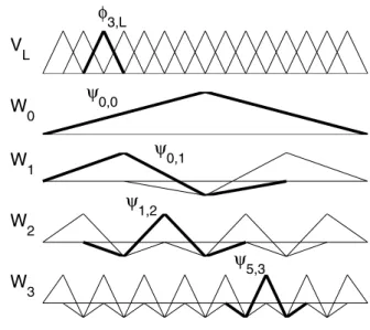
Fig. 1 Schematic of single-scale spaceVLand its decomposition into multiscale wavelet spacesW
single-scale basesΦL; for details see [36,44,94]. Denoting byWLthe span ofL,
the spacesVL+1admit a splitting
VL+1=WL⊕VL, L >0. (4.17)
Each wavelet spaceWLcan be thought of as describing the increment of information
when refining the finite element approximation fromVLtoVL+1. Furthermore, (4.17)
implies that for anyL >0 the finite element spaceVL can be written as a direct
multilevel sum of the wavelet spacesW, < L. Thus, anyuL∈VL=VN has the
representation uL= L−1 =0 j∈∇ dj,ψj,,
with suitable coefficientsdj,∈R. Figure1 illustrates the decomposition of the
fi-nite element spaceVL,L=4, spanned by continuous, piecewise linear (nodal) basis
functionsφi,Linto its increment spacesW,=0, . . . ,3, spanned by waveletsψj,.
In the multidimensional setting we obtain multivariate wavelet basis functions by using tensor products. The finite element spacesVLcan then be characterized by
VL=span
ψj1,1(x1)· · ·ψjd,d(xd):1, . . . , d≤L, ji∈ ∇i
.
Since these multivariate wavelet bases consist of products of one-dimensional wave-lets, they form hierarchical bases as in [61]. Thus, the spacesVLcan be replaced by
sparse tensor product spaces
ˆ VL=span ψj1,1(x1)· · ·ψjd,d(xd):1+ · · · +d≤L, ji∈ ∇i .
In [29,96] it is shown that, under certain smoothness assumptions on the solutionuof (4.12), the sparse tensor product spaces preserve the approximation properties of the full tensor product spaces while there holdsNˆ :=dimVˆL=O(N|logN|d−1)Nd.
Therefore, the complexity of the finite element stiffness matrix can be reduced to O(Nˆ2)instead of originallyO(N2d)non-zero entries.
Furthermore, wavelet basis functions give rise to certain cancelation properties and norm equivalences as illustrated in e.g. [21,36]. One therefore obtains sharp es-timates for the entries of the corresponding stiffness matrix, cf. [91,101]. Herewith a priori compression schemes can be defined that further reduce the complexity of the stiffness matrix. The compression exploits the fact that the position of large en-tries in the stiffness matrix arising from a model with jumps resembles the structure of a Black–Scholes stiffness matrix. The remaining entries can a priori be proved to be negligible. Therefore, the compression scheme (asymptotically) reduces the com-plexity of a model with jumps to that of the Black–Scholes model.
Combining the compression scheme with the sparse tensor product spaces results in a computational complexity ofO(N )ˆ instead of the originalO(N2d). It is proved that these wavelet schemes preserve stability and convergence of the classical finite element schemes, cf. [101–103].
Since the convergence of finite element methods has been studied intensively for many decades, sophisticated numerical analysis is available here. For example, in [50,101] it is shown that when using piecewise polynomial basis functions of degree p≥1, the finite element scheme described above converges at rate p+1 inx (provided sufficient smoothness of the solutionuof (4.4)). In particular, employing a piecewise linear basis as illustrated in Fig.1one obtains a second order scheme.
American options Similarly to the variational formulation for European contracts, for finite element implementation the partial integro-differential inequality (4.8) is reformulated into the corresponding variational inequality
Findu(τ,·)∈Kg˜τ:= v∈D(E):v≥ ˜gτa.e. such that ∂u ∂τv−u D(E)∗,D(E)
+E(u, v−u)≤0 a.e. in[0, T], for allv∈Kg˜τ,
withg˜τ given by (4.9).
Choosing finite dimensional subspacesVN ⊂V, as above, to discretize in space
and applying theθ-scheme defined in (4.16) withθ=1 to discretize in time leads to a sequence of matrix linear complementary problems (LCPs)
Givenu0, findum∈K:=v∈RdimVN:v≥ ˜g
t
such that for allv∈K, (4.18)
v−um+1(M+tA)um+1≥v−um+1Mum, m=0, . . . , M−1, with M, A as in (4.15) and whereu0denotes the coefficient vector ofu0. As already
described in (3.3) this discretization can be interpreted as approximating the value of the American option by a sequence of Bermudan option values.
For a large numberN of degrees of freedom, standard solution methods like pro-jected SOR [43] for the matrix LCP (4.18) are not suitable, since their rate of conver-gence depends onN. The wavelet-based solution algorithm suggested in [90] relies on a fixed point iteration where in each iteration step aVL-projectionPK onto the
convex coneK has to be realized. Due to norm equivalences of the wavelet basis, the outer fixed point iteration convergences at a rate independent of the number of degrees of freedom. The projectionPK is based on a wavelet generalization of the
classical Cryer algorithm [43].
5 Comparison
So far we have presented the setup and general methodology of the major numerical schemes for multidimensional Lévy models. In this final section we explain the main differences and problem-dependent advantages of these methods.
Admissible exotic contracts The applicability of the different numerical methods to exotic contracts in Lévy models is essentially subject to the same challenges as in the classical Black–Scholes model.
As we have already seen in the above sections, nowadays American contracts can be handled more or less efficiently by all described methods. For Monte Carlo however this was long thought to be an impossible task, since it is based on simulation forward in time. In mesh-based methods one employs backward time stepping. With this, the efficient pricing of American contracts is straightforward. Therefore, Monte Carlo schemes are still considered inferior to mesh-based methods when applied to American contracts.
Contracts with discontinuous payoffs such as digital options do not pose any addi-tional challenges for the finite element method, since it solves the variaaddi-tional problem (4.12), which isL2-based. Under certain conditions, however, discontinuous payoffs can result in a decreased rate of convergence for Monte Carlo methods; for details see e.g. [25].
Pricing of barrier options can be handled very easily with a PIDE-based approach, since one simply has to restrict the price-space domain of the discretization to that of the barrier and impose suitable boundary conditions. Here, very complex multidimen-sional barriers can be handled instantly. If the barrier is monitored continuously, pric-ing barrier options is somewhat more complicated for Monte Carlo methods, since we simulate forward in time and one cannot see what happens in between sampling dates. Therefore, straightforward Monte Carlo methods overestimate the prices of knock-out options and underestimate those of knock-in contracts. Correction tech-niques have been considered for several years now; see e.g. [8,28,106]. In the case where the barrier is monitored at discrete days (which is common in practice) one may choose the sampling dates to coincide with the observation dates and hence the bias in the Monte Carlo estimates vanishes. For Fourier methods the Wiener–Hopf factorization can be used; see e.g. [19].
Monte Carlo methods are easily applied to path-dependent derivatives such as Asian or lookback options, since sample paths are simulated forward in time and
the history at each time step is known. One only has to take into account that, as for barrier options, Monte Carlo methods might result in biased estimates if the con-tract is monitored continuously. Since mesh-based methods solve backward in time, they are intrinsically not well suited for path-dependent options. However, several methods have been introduced to provide PIDE-based tools for such contracts. For example, to price Asian options one may introduce an additional variable, i.e., in-crease the problem dimension, to handle the averaging of the underlying’s prices; see e.g. [119,123].
For all numerical methods, a continuously paid dividendq can simply be handled by changing the interest rater→r−q. If the dividend is paid at discrete points in time it can still be handled easily by Monte Carlo methods, since one is proceeding forward in time and payment of a dividend results in an immediate decrease of the underlying’s value. For Fourier and PIDE-based techniques the situation of discretely paid dividends is usually more complicated, since one needs to enforce additional no-arbitrage conditions; see e.g. [122].
Admissible market models Monte Carlo methods are applicable to any Lévy process Xas long as there is an efficient way of simulating its trajectories. Furthermore, the simulation techniques illustrated in Sect.2 provide a very general framework for Monte Carlo simulations applicable to more exotic models. Such simulations can however be rather involved for general multidimensional models. They have to be considered separately for each model.
In contrast to constructing a new simulation scheme for each process, PIDE-based methods provide a standard approach whenever the PIDE (4.4) admits a unique solu-tion and the Lévy measureνofX is available in a suitable form, i.e., if the density or tail integrals ofν are known explicitly. These requirements have been proved for all major one-dimensional models (see [40, 91]) and multidimensional Lévy cop-ula models (see [50,104]). One major advantage of the PIDE-based methods is that changing the market model only amounts to changing the stiffness matrix A in (4.15) and (4.16). The matrix A needs to be assembled only once for each model and can be re-used for different payoffs. PIDE-based methods are hence well suited for the analysis of model risk.
As long as the characteristic function is known (see [114] for an overview) Fourier methods using the fast Fourier transformation provide a very efficient standardized approach in moderate dimensions. Except for driving processes with independent marginals or subordinated Brownian motion, however, the characteristic function is generally not known in Lévy models of dimensiond >1.
Implementation It is well known that in the Black–Scholes setting one advantage of the Monte Carlo method is its intuitive and rather simple implementation. In fact for the one-dimensional Black–Scholes model also Fourier, finite difference and classical finite element methods can be implemented by straightforward standard techniques. A great amount of fundamental literature is available in this case; see e.g. [2,22,
115]. However, for (multidimensional) Lévy models more work is required for all methods. Even though the convergence rate of the Monte Carlo method is dimension-independent, its implementation in general requires special considerations for differ-ent techniques; see e.g. [117] for multidimensional simulation based on copulas.
As illustrated in the previous sections, all naive grid-based techniques such as standard Fourier and PIDE methods suffer from an exponential growth of complexity with the dimension. Applying sparse grids (cf. [29,50]) or the so-called multigrid technique (cf. [17,105]) to overcome this issue requires the implementation of a non-trivial data structure to handle the degrees of freedom efficiently. Furthermore, being the most general grid-based method, the implementation of wavelet-based finite elements requires additional handling of the compression techniques. For implemen-tation details see [124].
Model sensitivities and Greeks Calculating price sensitivities (e.g. the Greeks) is a central modeling and computational task for risk management and hedging. We distinguish two classes: Sensitivities of the priceV in (1.2) to variations of a model parameter, like the Greek Vega∂σV; and sensitivities ofV to variations of the state
space such as the Greek Delta∂SV. Mesh-based methods are known to be well suited
for the fast and accurate calculation of sensitivities whereas Monte Carlo methods are facing a certain challenge in this respect.
For PIDE-based methods, for instance, suppose the market model and hence the operatorA=ABS+AJ in (4.4) depends on some model parameter η. We want to
calculate the sensitivity of the solutionuof (4.4) with respect toη. To this end, write u(η0)for a fixed realizationη0of ηin order to emphasize the dependence ofuon
η0in (4.4). Then, as shown in [66], the derivativeu(δη)˜ ofuwith respect toη, i.e., ˜
u(δη):=lims→0+ 1s(u(η0+sδη)−u(η0)),is the solution of the PIDE
∂u(δη)˜
∂τ +A(η0)u(δη)˜ = −DηAu(η0), u(δη)(0,˜ ·)=0 inR
d,
whereDηAis the derivative ofAwith respect toη. Therefore, the derivative of u
with respect to η can be obtained as a solution of the same PIDE as the price u itself, where now the right hand side depends onu. Thus, sensitivities with respect to model parameters can be calculated with the same computational effort as the price itself. Furthermore, it is shown in [66] that all computed sensitivities converge with the same rate as the original priceu. For sensitivities with respect to a variation of the state space, a finite difference-like differentiation procedure is presented in [66] which allows to obtain the sensitivities from the finite element forward price with the same convergence rate but without additional work.
Using a similar approach, also Fourier methods are capable of calculating sensitiv-ities with respect to state space variation efficiently; see e.g. [4] for some numerical examples.
For Monte Carlo methods the computing time required for the calculation of sensi-tivities can be significantly greater than the time needed to calculate the prices them-selves (to the same accuracy). For example, suppose one wants to estimate the Delta ∂SV (S). Then, one can compute a Monte Carlo estimator forV (0, S+δ)for some
small perturbationδ. With this, the Delta∂SV (S) may then be approximated by a
forward finite difference estimator(V (0, S+δ)−V (0, S))/δ. In the Black–Scholes setting, it is proved in [60] that the best possible convergence rate for such an approx-imation isN−1/4 if the simulations of the two estimators are drawn independently