Durham Research Online
Deposited in DRO:
13 February 2018
Version of attached le:
Accepted Version
Peer-review status of attached le:
Peer-reviewed
Citation for published item:
Fan, L. and Coombs, W.M. and Augarde, C.E. (2018) 'The point collocation method with a local maximum entropy approach.', Computers and structures., 201 . pp. 1-14.
Further information on publisher's website:
https://doi.org/10.1016/j.compstruc.2018.02.008Publisher's copyright statement: c
2018 This manuscript version is made available under the CC-BY-NC-ND 4.0 license
http://creativecommons.org/licenses/by-nc-nd/4.0/
Use policy
The full-text may be used and/or reproduced, and given to third parties in any format or medium, without prior permission or charge, for personal research or study, educational, or not-for-prot purposes provided that:
• a full bibliographic reference is made to the original source • alinkis made to the metadata record in DRO
• the full-text is not changed in any way
The full-text must not be sold in any format or medium without the formal permission of the copyright holders. Please consult thefull DRO policyfor further details.
The point collocation method with a local maximum entropy
approach
Lei Fan∗, William M. Coombs, Charles E. Augarde
Department of Engineering, Durham University, Lower Mountjoy, South Road, Durham, DH1 3LE, UK
Abstract
Meshless methods have long been a topic of interest in computational modelling in solid mechanics and are broadly divided into weak and strong form-based approaches. The need for numerical integration in the former remains a challenge often met by using a background mesh or complex stabilised nodal approaches. It is only strong form-based point collocation methods (PCMs) which dispense with meshing and integration entirely, and for this reason PCMs remain of interest. In this paper, a new point collocation method is developed which is based on maximum entropy basis functions which bring benefits in terms of accuracy and efficiency. These basis functions possess non-negativity and a weak Kronecker delta property which decreases the errors on boundaries to im-prove overall accuracy of solutions. After a discussion of implementation issues in the new method, numerical examples are presented, including 1D and 2D problems with linear elasticity and Poisson PDEs, on both convex and non-convex domains to show the performance. Comparisons of con-vergence properties with respect to accuracy and computational cost (both CPU time and floating point operations) are made with an existing method, the reproducing kernel collocation method (RKCM), to show the effectiveness of the MEPCM. In all examples, higher order convergence rates are obtained using the developed method with increasingly reduced computational effort for higher levels of accuracy due to the fundamental advantages.
Keywords: Point collocation; local maximum entropy; reproducing kernel particle; solid mechanics.
∗Corresponding author. Tel.:+44 0 787 432 6770. Email address: [email protected](Lei Fan )
1. Introduction
Computational solid mechanics has been dominated by methods based on weak forms for decades, the prime examples being the finite element method (FEM) and the boundary element method (BEM). Many of the difficulties met in using these weak form methods relate to the need for the problem domain to be discretized into a mesh; the generation of the mesh may itself be a ma-5
jor computational problem in 3D, while the performance of a mesh during a non-linear analysis can deteriorate due to distortion. Meshless weak form-based methods, developed since the 1990s, have been seen as a potential solution to this problem (for a comprehensive review, refer to [1]) and include the element-free Galerkin method (EFGM) [2, 3], the Meshless Local Petrov-Galerkin method [4] and reproducing kernel particle methods (RKPMs) [5]. These weak-form based mesh-10
less methods have been successfuly used to model problems involving large deformations [6], crack propagation [7, 8, 9, 10] and non-linear materials [11, 12]. Despite many positive aspects such as improved accuracy, weak-form based meshless methods have yet to rival finite elements in commer-cial codes largely due to their computational cost. In addition, some meshless methods have been criticised for not actually being truly meshless as a background grid is needed for integration. To 15
counter this criticism, direct nodal integration has been developed (e.g. [13]) and some of the initial issues with instability and low accuracy have been addressed, such as in the stabilized conforming approach in [14].
Strong form-based meshless methods based on point collocation offer the possibility of mesh-free methods with low computational cost and have in the past been labelled as “truly meshless” 20
[15, 16, 17, 18, 19]. They are straightforward to implement and remove entirely the complexities associated with domain integration [20, 21]. These methods discretize a problem domain into collocation (or “data”) points at which the PDE is approximated using basis functions associated with a different set of points (the source points or “centres”). Boundary conditions are imposed directly on boundary points and a linear system is derived in which the field variable values at source 25
points are the initial solution. An early example of this type of method is due to Kansa [15, 16] who employed radial basis functions (multiquadrics) and in later work, a radial basis collocation method was used to solve singularity [22], and higher order problems [23]. More recently, other meshless collocation methods have been proposed such as schemes with the moving least squares basis for solutions to the incompressible Navier-Stokes (NS) equations in the velocity-pressure formulation 30
and multiple complex-geometry problems in 2D [25]. However, the condition number of the discrete system formed using radial basis function-based collocation was found to be large and additional approaches [26] have been developed to address this ill-conditioning problem. Alternative strong form collocation frameworks have been used to solve problems defined by PDEs using basis functions 35
obtained by the reproducing kernal approximation [27], where the method is generally referred to as the reproducing kernel collocation method (RKCM). RK-based methods automatically satisfy consistency requirements (similar to completeness in finite elements) assuring algebraic convergence rates [28, 29]. While isogeometric methods are usually associated with finite elements, they have made an appearance in collocation methods, first in [30], the aim being to exploit the smoothness 40
properties of NURBS-based basis functions. Different methods are proposed for the generation of optimal locations for collocation points in these methods in [31] and the computational efficiency of these methods is compared with Galerkin methods in [32].
It is important to note that in strong form point collocation methods (PCMs), higher deriva-tives of the basis functions are required than would typically be the case, for the same problem, in 45
a weak form-based method such as the EFGM. Although approximation schemes such as moving least squares (MLS) and reproducing kernels are smooth, the analytical determination of higher derivatives required for PDEs such as elasticity are complex, and their step-by-step calculation is time-consuming. Basis functions derived using the standard RKPM require the inversion of mo-ment matrices (as do equivalent MLS-based functions). This inversion feature complicates matters 50
when calculating basis function derivatives to first and second order especially in multidimensional problems, increasing the computational cost. Evidence of this can be found in [33, 34] and to address it, some novel formulations have been devised such as a gradient RKPM [35] where the calculations of the basis function derivatives are simplified, differential reproducing kernel interpo-lation (DRK) [36, 37] and a fast MLS approach [38] in which novel efficient algorithms are used to 55
enhance the efficiency of the derivative calculations. Another source of computational cost comes from the observation that for optimal convergence more collocation points than source points are required, forming an overdetermined system [35, 21] which must be solved in, say, a least squares sense rather than directly. Despite these shortcomings, the RKCM is straightforward to implement and has been an important tool for the analysis of engineering problems [39, 40]. However, numer-60
ical results sometimes suffer from instability and accuracy issues. A key contributor to these errors is in the imposition of essential boundary conditions [41], as is the case with MLS and RK-based
meshless methods of all types.
In this paper, we tackle the latter source of error by making use of maximum-entropy (max-ent) basis functions. These are derived from classical information theory [42] and the max-ent principle 65
[43]. Two key characteristics of max-ent basis functions are non-negativity and the satisfaction of the weak Kronecker-delta property on the boundaries. The former property makes the approximation schemes non-negative (convex) [44] and the max-ent basis functions smoother in contrast with other basis functions with negative values. The latter facilitates the imposition of essential boundary conditions accurately because the Kronecher-delta property on the boundary points makes the 70
essential boundary fully satisfied. In this case “weak” means that the max-ent basis functions for points inside the domain do not possess the Kronecker-delta property [45]. Max-ent basis functions with compact support are derived using weight functions [46] in which the first and second order reproducing conditions are viewed as constraints. The resulting approximations retain the same order of reproducing conditions, namely the first and second order max-ent basis functions [44, 47]. 75
Reviews of weak form-based meshless methods using max-ent basis functions can be found in [48, 49, 50, 51]. Max-ent basis functions are also used to couple the FEM and the EFGM in [52]. With the satisfaction of a weak Kronecker-delta property in max-ent basis functions, the imposition of essential boundary conditions can be carried out directly. There remain some issues with the imposition of Neumann boundary conditions, however, because the Lagrange multiplier in 80
the expression of the first max-ent basis function derivatives blow up for points on the Neumann boundary conditions which makes the first derivative values indeterminate [53]. This is an open problem beyond the scope of this paper. As indicated above, max-ent approximation has only been used to date for weak form-based meshless methods and in this work, local max-ent basis functions are used in a simple PCM. Considerable computational efficiency is demonstrated for the presented 85
method as compared to a PCM based on RK basis functions.
The structure of this paper is as follows. Section 2 provides a brief review of the basic theory of PCMs, the expressions for local max-ent basis functions and their derivatives. Implementation issues associated with the max-ent PCMs are presented in Section 3. In Section 4, the proposed method is applied to some numerical examples to validate the approach. Final remarks are collected 90
2. Background
2.1. Review of point collocation methods
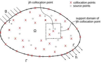
The theoretical background now presented is based on two-dimensional spatial domains but it is straightforward to modify for other dimensionalities. Consider a two-dimensional problem domain Ω bounded by boundary Γ (Γ = Γu∩Γt) as shown in Figure 1. The collocation points and source
Figure 1: A problem domain with boundary conditions in PCMs.
points (numberingNcandNsrespectively) are distributed in the domain Ω and on the boundary Γ. The collocation points are distributed to enforce the governing PDE and corresponding boundary conditions which are satisfied at each collocation point. The surrounding source points, which fall in the local support domain of each collocation point, are used for the construction of the basis functions and determine the approximation of the solution over the domain. The governing PDE and the two types of boundary conditions are described as
Lu=fb inΩ, (1a)
Luu=g onΓuand Ltu=h onΓt, (1b)
collocation points,g is the prescribed value on Dirichlet (essential) boundaries Γu and hdenotes the known traction on Neumann (natural) boundaries Γt. To implement the PCM one imposes the appropriate condition from Eqn (1) at each collocation point, leading to a discrete set ofNc equations which are in block matrix form
K11 K12 · · · K1Ns K21 K22 · · · K2Ns · · · · KNc1 KNc2 · · · KNcNs u1 u2 · · · uNs = f1 f2 · · · fNc . (2)
In Eqn (2), for the 2D elasticity case, eachKijis a 2×2 matrix with non-zero terms where collocation
pointihas source point j in its support. Vectors uj andfi are both 2×1. Entries in the Kij are
95
the appropriate differential operator applied to basis function values at each of thej source points in the support domain of the collocation point.
The size of the coefficient matrix in Eqn (2) is 2Nc×2Ns in 2D and whenNc =Ns a square system is formed that has a unique solution. However, whenNc > Ns (which is usually the case for reasons mentioned above) an over-determined system is obtained and a suitable solver (e.g. the least squares method) is employed to obtain the source point values. The field variable at any point can be evaluated by uh(x) = Ns∗ X j=1 φjuj, (3)
whereuh(x) is an approximation of the solution at any point,Ns∗ is the number of source points in support at the point andφj is the basis function associated with thejth source point.
2.2. Generation of basis functions using max-ent schemes
100
In this paper, a max-ent scheme [42] is used instead of MLS and RK methods to construct the basis functions. MLS and RK basis functions are employed in most early strong form-based meshless approaches but they are not strictly positive and do not possess the Kronecker-delta property. Additional effort is therefore required to impose Dirichlet boundary conditions and to keep the polynomial interpolants passing through collocation point values [54]. Max-ent basis functions are 105
strictly valid on convex domains (but function well on non-convex domains in many cases [55, 56]) and, importantly, possess the Kronecker-delta property on the boundaries, which facilities the direct
imposition of the essential boundary conditions and, as will be shown, leads to greater accuracy for a given discretization.
The maximum entropy idea arises from probability theory where a set of mutually independent events{A1, A2, ..., An}with unknown probabilities{p1, p2, ..., pn}, respectively, are considered. The
least biased probability distribution can be obtained by maximizing the informational entropyP(·) (the specific description of uncertainty) as
maximizeP(A1, A2, ..., An) =P(p1, p2, ..., pn) =− n X a=1 palogpa . (4)
If one replaces the probabilities by basis functions in a given defined domain then it is easy to see that the partition of unity property is obtained. The basis functions are obtained by combining the max-ent constraint expressed in Eqn (4) with the required linear reproducing conditions [46] and a weight functionwi to give compact support, i.e. maximising
P(φ, w) =− Ns∗ X i=1 φilog φi wi (5)
subject to (in the 1D case)
Ns∗ X i=1 φi= 1 and Ns∗ X i=1 φixi =x. (6)
The local max-ent basis functions derived this way can be written as
φi(x) =Zi Z (7) where Zi=wie−λi(xi−x) (8) and Z= Ns∗ X i=1 Zi, (9)
and Ns∗ is the number of source points in the support domain at each collocation point and λ
found via a Newton process [47] as
λ(x) =arg min logZ(x, λ). (10)
A detailed explanation of max-ent basis functions and their implementation can be found in [57]. The choice of weight function is to some extent arbitrary since there is no rigorous mathematical proof available at the moment to judge which type of weight function is better than another. In the problems covered in this study, the highest order required are second derivatives so an appropriate choice here for the the weight function is a cubic spline
w(r) = 2 3−4r 2+ 4r3 0< r≤ 1 2 4 3−4r+ 4r 2−4 3r 3 1 2 < r≤1 0 r >1 , (11) where r= kx−xik dm , (12)
is the normalized radius of the support domain anddmis the size of the domain of support at each collocation point, which is a user-defined parameter here taken as
dm=dmaxdx. (13)
where the scaling parameter dmax is typically 2.0−4.0 [58] and dx is the distance between the 110
collocation point and the nearest source point in its support domain. Sufficient source points are required in the domain to avoid matrix singularity problems, and the accuracy of the approximation at any point also depends on the scaling parameterdmax.
As indicated above, PCMs usually require expressions for derivatives of higher order than re-quired for weak form-based methods. The first derivatives of the max-ent basis functions [57] can be expressed as ∇φi=φi n (xi−x)T[H−1−H−1 Ns∗ X k=1 φk wk (xk−x)⊗ ∇wk] + ∇wi wi − Ns∗ X j=1 φj ∇wj wj o (14)
whereHis the Hessian matrix given by H= Ns∗ X k=1 (xk−x)⊗(xk−x)⊗φk, (15)
where ⊗ is the dyadic product of two vectors, for example, for any two vectors x⊗y = xyT. Similarly the second derivatives of the max-ent basis functions are
115 ∇∇φi = ∇φi⊗ ∇φi φi + φi n −H−1+ (xi−x)· ∇H−1+ h Ns∗ X k=1 φk wk (xk−x)⊗ ∇wk iT H−1o − φi n (xi−x)· ∇H−1 h Ns∗ X k=1 φk wk (xk−x)⊗ ∇wk i + h(xi−x)TH−1 i · ∇ Ns∗ X k=1 φk wk (xk−x)⊗ ∇wk o + φi n ∇∇wi wi − N∗ s X j=1 ∇wj wj ⊗ ∇φj− N∗ s X j=1 φj∇∇wj wj o (16)
The derivation of this second derivative is given in Appendix A.
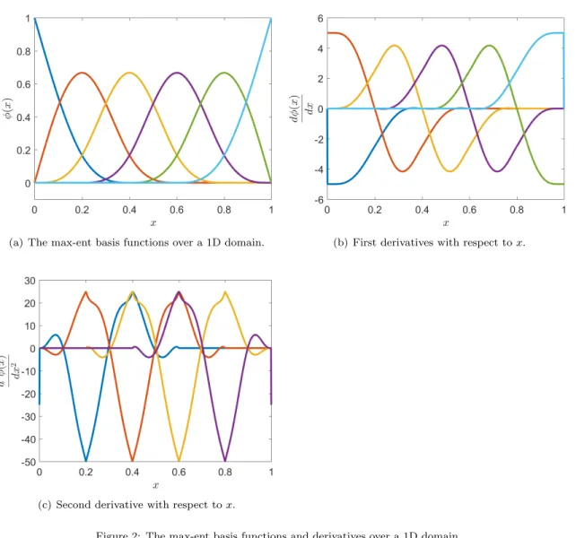
In Figure 2(a), the max-ent basis functions are plotted over a 1D domain, where 6 points are located at x = 0,0.2,0.4, . . . ,1.0. It can be seen that the max-ent basis functions possess non-negativity at all points and the weak Kronecker-delta property at the two boundary points which allows direct imposition of the essential boundary conditions. The first and the second derivatives of 120
the max-ent basis functions at each point in the domain are shown in Figures 2(b) and 2(c). Of note is the fact that the second derivatives of the max-ent basis functions are sensitive to the position of the points and distributing the collocation points and source points at the same positions may lead to serious defects with the numerical results because of the obtained values of basis function second derivatives. This will be discussed in the following section.
(a) The max-ent basis functions over a 1D domain. (b) First derivatives with respect tox.
(c) Second derivative with respect tox.
3. Implementation issues
3.1. A max-ent point collocation method (MEPCM)
In this section, some implementation issues associated with the proposed strong form point collo-cation approach (called the MEPCM from here on) will be discussed. The differential operators needed for the numerical examples in the following section are given here, all of which are for 2D spatial domains. The differential operators for a 2D Poisson problem are
∂2u ∂x2 + ∂2u ∂y2 =fb in Ω, (17a) u=g on Γu and ∂u ∂x+ ∂u ∂y =h on Γt. (17b)
noting that the field variableuis a scalar. For the MEPCM the differential operators which appear in Eqn (1) for the Poisson problem are therefore
L = ∂ 2 ∂x2 + ∂2 ∂y2, (18a) Lu= 1 and Lt= ∂ ∂x + ∂ ∂y. (18b)
For linear elasticity with small deformations the required differential operators are more compli-cated. Consider an elastic solid in 2D with material properties of Young’s modulus,Eand Poisson’s ratioν, with the domain Ω and boundary Γ (Γ = Γu∪Γt). Taking σ as the Cauchy stress tensor andfb as the body force, the equilibrium equation is
∇ ·σ=fb in Ω. (19)
Using the standard relation between strain and small displacements, and the constitutive law be-tween Cauchy stress and strain with the assumption of plane strain the first differential operator in Eqn (1) is L = E(1−ν) (1 +ν)(1−2ν) ∂2 ∂x2 + 1−2ν 2(1−ν) ∂2 ∂y2 1 2(1−ν) ∂2 ∂x∂y 1 2(1−ν) ∂2 ∂x∂y ∂2 ∂y2 + 1−2ν 2(1−ν) ∂2 ∂x2 . (20)
Along the Dirichlet boundary Γu, the boundary condition is given as
u=g. (21)
whereg are prescribed displacements, the relevant differential operatorLu is
Lu= 1 0 0 1 . (22)
The Neumann boundary condition is described as
σ·n=h, (23)
where nis the unit normal vector to the Neumann boundary and his the applied traction. The final differential operatorLtis given as
Lt= E(1−ν) (1 +ν)(1−2ν) ∂ ∂xnx+ 1−2ν 2(1−ν) ∂ ∂yny ν 1−ν ∂ ∂ynx+ 1−2ν 2(1−ν) ∂ ∂xny 1−2ν 2(1−ν) ∂ ∂ynx+ ν 1−ν ∂ ∂xny 1−2ν 2(1−ν) ∂ ∂xnx+ ∂ ∂yny . (24)
Substituting these differential operators into Eqn (1), the expanded form of the linear system is
Lu11 Lu12 · · · Lu1Ns Lu21 Lu22 · · · Lu1Ns · · · · LuNg1 LuNg2 · · · LuNg Ns Lt11 Lt12 · · · Lt1Ns Lt21 Lt22 · · · Lt2Ns · · · · LtNh1 LtNh2 · · · LtNhNs L11 L12 · · · L1Ns L21 L22 · · · L2Ns · · · · LNd1 LNd2 · · · LNdNs u1 u2 · · · uNs = g1 g2 · · · gNg h1 h2 · · · hNh fb1 fb2 · · · fbNd , (25)
whereNg,NhandNd are the numbers of collocation points at Dirichlet and Neumann boundaries and in the problem domain respectively (Ng+Nh+Nd =Nc). In this section, the explicit forms of operators for both 1D and 2D problems have been obtained and they will be next used to form 130
the strong form-based final linear systems.
3.2. The generation of collocation and source points
In previous papers on PCMs, there are examples of the use of regular and random distributions of points being used [59]. In this paper, we define a parameterαp as the ratio of Nc and Ns where
αp≥1. If the positions of collocation points coincide with source points, there are defects at these 135
coincident points in the second derivatives; the second derivative values at these coincident positions become very close to zero which is inconsistent with the analytical values and which then has an effect on the accuracy of the results. The smoothed second derivatives of the basis functions can be obtained as shown in Figure 2(c) when collocation points and source points are distributed at different positions. The reason for this can be seen by examining the second derivatives of the basis 140
functions where both(xi−x) and∇φiare zero when the points are coincident. In order to calculate the second derivatives of the max-ent basis functions properly, and to ensure the consequent stability of the solutions in the MEPCM, any superposition of points should be avoided andαp should be greater than 1. In the following examples, collocation and source points are distributed at different positions and the number of collocation points is one greater than the number of source points in 145
two directions.
4. Numerical examples
In this section, some simple numerical examples are used to demonstrate the efficiency and accuracy of the proposed MEPCM. In order to study the performance of the Kronecker-delta property on the boundary points, only essential boundary conditions are considered in the following examples. As mentioned above, there are issues in imposing Neumann boundary conditions which will not be considered in this paper although some additional constraints (conditions) could be employed in the calculations and different distributions of source points and collocation points may be devised that avoid the instability [53]. All examples presented have exact solutions so that clear error norms can be calculated to show convergence rates and computational performance. In the results presented
below the L2 error norm is used to assess error (being an appropriate measure for the types of
problems considered as discussed in [31]) and is evaluated as
e= ||u h−ue|| 2 ||ue|| 2 , (26)
whereuhdenotes the approximation to the field variable anduethe exact solution (scalar or vector). In the following examples, plots of L2 norms of relative error in the primary variable of solution
versus degrees of freedom are employed to demonstrate the rate of convergence of the method. The 150
efficiency of the proposed method will be shown compared to the RKCM. The detailed source of the RKCM formulations used in this paper can be found in [17].
4.1. 1D bar problem
The first problem is a 1D linear elastic bar of unit length fixed at a pointx= 0 and subjected to a body forcex. For a 1D problem, the linear system is set up so that the collocation points at the two ends satisfy the displacement boundary conditions and all collocation points inside the domain are then set to satisfy the governing equations. The analytical solutions for the displacement and stress field of this 1D bar problem are
u(x) = 1 E 1 2x− x3 6 and σ(x) =1−x 2 2 , (27)
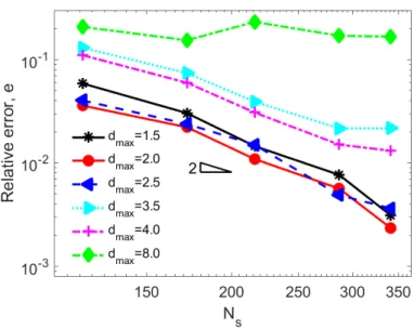
where here, E = 1.0. The unit length bar is discretized by a uniform distribution of collocation points with source points located between each pair of collocation points as shown in Figure 3. The 155
figure also shows sizes of the support domains for two different values of dmax. To demonstrate the effect of the choice ofdmaxon accuracy, the problem has been solved using the MEPCM with a range of values of this parameter, for varying discretizations (Ns values), and the results are plotted in Figure 4. In analyses with dmax = 1.5,2.0,2.5 each collocation point has two source points in support, however the accuracy and convergence properties differ between analyses due 160
to the the effect ofdm in Eqn (13) on the weighting functions embedded in the basis functions in Eqn (11). In this problem the optimum dmax is around 2.0 with close to quadratic convergence characteristics for all three analyses. When dmax is increased to 3.5, 4 and 8 the accuracy and rate of convergence deteriorate, likely due to the loss of locality of the approximation (as seen in MLS as it moves towards LS). It is particularly noticeable that the convergence rate fordmax= 8.0 165
Figure 3: A portion of the 1D bar with different sizes of support domain.
is very poor. From this discussion, it clearly remains difficult to predicta priori optimum values ofdmax although as a linear basis is used to construct the max-ent basis functions, the minimum number of source points in support is 2, which provides a lower bound value fordmax. As discussed in Section 3, source points and collocation points should not be distributed at the same positions. When analyses are carried out with coincident points, theL2 norms of displacements are recorded 170
as 0.4929, 0.4936, 0.4942, 0.4943, 0.4936, 0.7581 withNc=Ns=119, 172, 287, 341, 1000, 2000. It is clear theL2 norms do not converge using coincident source points and collocation points.
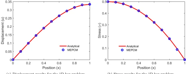
Figures 5(a) and 5(b) compare the MEPCM results from the “best” choice of dmax(= 2.0), with Ns = 200 and Nc = 201, with the analytical solution, showing close agreement (note that for clarity only 11 MEPCM results have been plotted from the 201 total values). The absolute 175
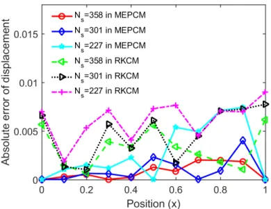
displacement errors at 11 selected collocation points using the MEPCM and the RKCM are shown in Figure 6 for different refinements. It is clear that the boundary conditions can always be imposed accurately in the MEPCM due to the Kronecker-delta property at boundaries of the max-ent basis functions. While in the RKCM, the displacement errors on two edge points are greater than 0.005 which has a major effect on the totalL2 norm of displacement error for the whole problem. Since 180
the problem is non-symmetric, it is reasonable that the errors at two ends using the RKCM are different. The convergence rates using the two methods are shown in Figure 7 in whichNsdenotes
(a) Displacement results for the 1D bar problem. (b) Stress results for the 1D bar problem. Figure 5: 1D bar problem predictions compared to the analytical solution.
Figure 6: The displacement errors for the 1D bar problem with differentNs.
in the case of the MEPCM as compared to the RKCM. In PCMs, errors can be attributed to
Figure 7: Error convergence rate for the 1D bar problem.
boundary errors and domain errors. For the RKCM, the combination of the two effects mentioned 185
Figure 8: Convergence rate of strain energy for the 1D bar problem.
reduced leading to better convergence rates. In Figure 7, the errors at boundary points and in the domain are split out and theL2norm of relative error in the domain for refinements are presented.
In the MEPCM, the convergence rates for the whole problem and for the domain alone match because of the accurate imposition of the boundary conditions. Using the RKCM, the L2 norm 190
for the problem domain alone is smaller than the L2 norm for the whole problem and keeps the
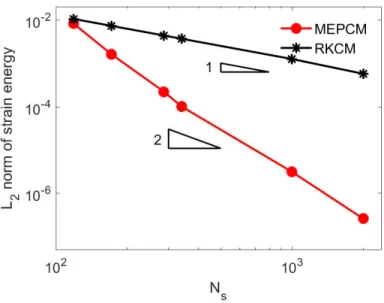
same convergence rate as the whole problem. In Figure 8, the L2 norms of strain energy using
both the MEPCM and the RKCM are compared. Comparing Figure 7 and 8, a similar trend is obtained for the L2 norm of displacement and strain energy. This is a clear demonstration
of the major improvement the max-ent approach gives to the MEPCM in terms of reducing the 195
error associated with imposing the boundary conditions. For the 1D bar problem, comparing accuracy and convergence using the MEPCM and the weak-form based formulation in [57], both are better in the weak-form based method. With “strong” and “weak” form-based methods, the fundamental difference lies the approximation. In strong formulations, all provided information located at the discrete collocation points. All connectivities between points are avoided to decrease 200
the complexities. However the weak form approximation is an average value over an integral domain which is likely to be richer than a collocation approach with the same number of points. In this case, unlike in [57], a high number of collocation points and source points are distributed in the
whole domain and on the boundaries using the MEPCM to study the convergence performance. The information at each collocation point only represents the collocation point itself rather than the 205
average value over its integral domain. In the comparison between the strong-form based methods (the MEPCM and the RKCM) and the weak-form based method in [57], the MEPCM and the RKCM have lower convergence rates.
Computational cost is clearly of great importance for numerical methods applied to challenging real world problems in terms of reducing the error associated with imposing the boundary condi-210
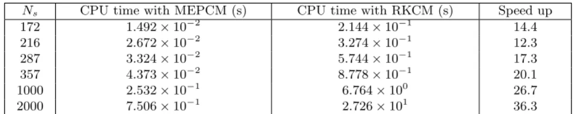
tions. Both the MEPCM and the RKCM programs in this paper run in MATLAB R2015b using the Intel(R) Core(TM) i7-4790 CPU @ 3.60 GHZ. Table 1 gives CPU times for both methods for selected analyses, varying the discretization. The results show that for a given discretization, the MEPCM leads to lower CPU times than the RKCM in all cases, and from the results discussed above concerned with convergence, it can be concluded that the MEPCM gives greater accuracy 215
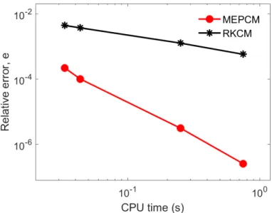
in a lower CPU time. Further support for this point can be shown by plotting error against CPU time as in Figure 9 where the advantage of the MEPCM is obvious. The computational cost of the
Figure 9: Convergence of displacement error with CPU time.
two methods is principally concentrated in the construction of the basis functions and derivatives, and in the solution of the linear system. Both max-ent PCM and RKCM have similar overheads
Ns CPU time with MEPCM (s) CPU time with RKCM (s) Speed up 172 1.492×10⁻² 2.144×10⁻¹ 14.4 216 2.672×10⁻² 3.274×10⁻¹ 12.3 287 3.324×10⁻² 5.744×10⁻¹ 17.3 357 4.373×10⁻² 8.778×10⁻¹ 20.1 1000 2.532×10⁻¹ 6.764×100 26.7 2000 7.506×10⁻¹ 2.726×101 36.3
Table 1: CPU times for the MEPCM and RKCM in the 1D bar problem.
the RKCM, the inversion of the moment matrix and the calculation of the derivatives step by step are both complicated and time-consuming. The chain rule is used to derive the second derivatives of RKPM basis functions and the second derivatives of all terms in the RKPM formulation are required which is costly especially for the second derivatives of the inverse of the moment matrix. However, these calculations are totally avoided with max-ent basis functions, and the only poten-225
tial issue is the determination of the Lagrange multipliers λi by the Newton process because the derivatives of the max-ent basis functions are derived analytically. In this elasticity example on which the proposed MEPCM has been tested to date, the max-ent schemes have better accuracy for a given discretisation than those based on RK methods.
Another useful metric in comparisons of numerical algorithms is floating point operations (flops). 230
Ideally one should be able to make clear comparisons of methods, such as between the MEPCM and the IGA methods in [31]. In some cases it is possible to break down a complex algorithm to provide neat expressions for the order of flop counts related to the discretization (e.g. the number of elements in the IGA methods), dimensionality and order of basis (e.g. Table 2 in [31]). Both MEPCM and RKCM form the linear system of equations at collocation points in the same way 235
as the IGA-C method of [31] so we expect flop counts for those operations to be similar here. However, attempting to go further with the MEPCM and RKCM methods, encounters problems in that there is no clear link between the underlying basis (which is linear here) and the order of the computed basis functions developed via the max-ent procedure (for MEPCM at least) which is undefined. Instead we present results to indicate trends as regards flop counts based on numerical 240
experiments.
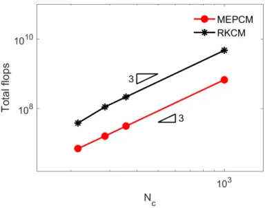
The total flops required for instances of the 1D problem, with different discretizations, are plotted in Figure 10. The figure shows that for the same number of collocation points, the flop count using the MEPCM is smaller than the RKCM. For this 1D problem, the total cost (if taken
proportional to flop count) for both MEPCM and RKCM isO(N3
c). It is hard to determine the role 245
of the dimensionality here and, for the reasons outlined above, not possible to include the order of a basis. In any case, comparisons between the IGA methods and the methods presented here are not possible with overall flop counts as those data are not presented in [31].
Figure 10: Total flops for analysis againstNc.
Maintaining interest in flop counts but now focussing on comparison of the MEPCM with the RKCM it is instructive to consider the cost of forming the basis functions in each. In the formation 250
of the max-ent basis functions, the flops per Newton iteration are the same for each collocation point in the same discretization although the number of iterations is not known in advance. The cost of constructing max-ent basis functions with varyingdmax is shown in Figure 11(a) in which the gradients of all the lines are close to 2 for differentdmax. The costs of constructing the max-ent and RKPM basis functions and derivatives are shown in Figure 11(b) where it is clear that the flop 255
counts for max-ent basis functions are less than the RKPM basis functions. It is also observed that the cost of calculating RKPM basis functions derivatives is more expensive than the max-ent basis functions derivatives because some variables calculated in the max-ent basis functions can be reused in the calculation of the max-ent derivatives. The cost of calculating the max-ent and RKPM basis functions in terms of the number of collocation points is seen to beO(N2
c). Switching to a 2D 260
(a) Flops of max-ent basis functions with differentdmax. (b) Flops of the basis functions and derivatives. Figure 11: Computational cost of constructing the basis functions and derivatives 1D problem.
Figure 11(b) for 1D and indicates the same relation for 2D as in 1D problem, implying that the basis function formation is not controlled by dimensionality. A further plot of flops against the reciprocal of distancehbetween two nearest collocation points for a regular distribution (in Figure 12(b)) gives gradients close to 4. As for the 1D problem, the flop count in terms ofNc is equivalent 265
to the flops in terms of 1h considering the proportional relation betweenNc and h1 in 1D. Therefore, the cost for constructing the max-ent and RKPM basis functions is conjectured to be O((1h)2d) wheredis the dimension of the physical problem. Finally it is clear that in all cases, the MEPCM is better than the RKCM.
4.2. 2D Poisson problem
270
The second example is a 2D Poisson problem with Dirichlet boundary conditions on a unit square domain. The governing equation is
(a) Flops of the basis functions and derivatives. (b) Flops of the basis functions and derivatives against 1/h. Figure 12: Computational cost in a 2D domain.
with the following Dirichlet boundary conditions
ux=0=y2 (29a)
ux=1= 1 +y2 (29b)
uy=0=x2 (29c)
uy=1=x2+ 1, (29d)
where the analytical solution is
u(x, y) =x2+y2,Ω∈(0,1)×(0,1). (30)
The collocation and source points are distributed in thexandy directions as described above and the scaling parameter of the support domaindmaxfor each collocation point is 2.0. Note that for a 2D Poisson problem, there is a single degree of freedom in the field variable at each collocation and also that the PDE contains no mixed derivatives, which simplifies the formation of the differential operator, as compared to elasticity. For this example, four different refinements were used (Ns=121, 275
Nc=144;Ns=441,Nc=484;Ns=1681,Nc=1764;Ns=2601,Nc=2704) andNs1/2 denotes degrees of freedom since the approximation to the field variable is a scalar at each collocation point in this
2D Poisson problem. Figure 13 shows convergence rates for the MEPCM and the RKCM for this problem, in which the MEPCM clearly performs better than the RKCM. The differential operators in 2D Poisson problems are simple andxandycomponents are independent without the coupling 280
effect which simplifies the implementation of the governing equation and reduces the relative error. Table 2 gives the computational times of the MEPCM and the RKCM analyses for this problem,
Figure 13: Error convergence rate for the 2D Poisson problem.
and again, the advantage of the former is clear. The corresponding ratios for CPU time vary from 2.7 (Ns = 121) to 10.8 (Ns= 2601). Compared with the 1D bar problem, these simulations take longer since the calculation of basis functions and the derivatives in two directions are required and 285
the linear solver will also be consuming more CPU time than the 1D problem, despite the change in PDE. The speed up is lower in the first example which may also be explained by the discretization. In a 2D domain, the distribution of points is known to have an effect on the iteration times in the calculation of the Lagrange multipliersλi and hence the overall computational time. Although this speed up is not as significant as seen in the 1D bar problem, it is nevertheless the case that the 290
MEPCM is more efficient than the RKCM for this problem and that the speed up increases with refinement.
Ns CPU time with MEPCM (s) CPU time with RKCM (s) Speed up
121 5.467×10⁻² 1.476×10⁻¹ 2.7 441 2.290×10⁻¹ 7.755×10⁻¹ 3.4
1681 2.100×100 1.329×101 6.3
2601 6.295×100 6.794×101 10.8
Table 2: CPU times of the MEPCM and RKCM analyses of the 2D Poisson problem.
4.3. A 2D elasticity problem: a confined square domain
The third example is a linear elastic unit square domain, subjected to Dirichlet boundary conditions (rollers on three sides and a prescribed displacement on the fourth) as shown in Figure 14. The purpose of this numerical example is to study the performance of the elasticity problem with convex and symmetric geometry and essential boundary conditions using the MEPCM. The analytical
Figure 14: An elasticity problem: a confined square domain subjected to a displacementv= 1 in theydirection.
solution for the displacement field for this problem is simply
u= 0 and v= 1−ν
2
E y , (31)
For 2D linear elasticity, the differential operators are stated above, in Eqns (20), (22) and (24) where the field variable is the 2D displacement vector. The material properties used are Young’s modulus 295
used to plot the convergence rates in Figure 15. In 2D elasticity problems, (2×N s)1/2 denotes
degrees of freedom given that the approximation of the field variable is a 2×1 vector. The results
Figure 15: Error convergence rate for the 2D elasticity problem: a confined square domain.
again demonstrate that, for a given level of discretization, the error in the MEPCM is less than 300
that in the RKCM. In addition, the convergence rate in the MEPCM is better. In this example, the differential operators for elasticity problems are more complicated than for the 2D Poisson problem. Another feature in this 2D elasticity problem is that the mixed second derivatives of the basis functions ∂x∂y∂2φ are required in the differential operators thusxandy directions are coupled. In this example, the geometry and boundary conditions are symmetric and the body force for this 305
elasticity problem is zero which simplifies the implementation. The CPU times for solutions using both methods are given in Table 3 and again there appear to be clear benefits using the MEPCM. The speed up increases with an increasing number of source and collocation points. At the same time, however, the overall computational time in this 2D elasticity problem is longer than for the previous 2D Poisson problem, for similar discretizations. The explanation for this is the need for 310
calculation of mixed derivatives of max-ent basis functions, assembly of the larger final coefficient matrix and the least squares solver for the over-determined system in this example, all of which take more time than the 2D Poisson problem.
Ns CPU time with MEPCM (s) CPU time with RKCM (s) Speed up
121 8.200×10⁻² 2.010×10⁻¹ 2.5
441 3.392×10⁻¹ 1.176×100 3.5
1681 3.150×100 2.553×101 8.1
2601 9.099×100 8.560×101 9.4
Table 3: CPU times for analyses using the MEPCM and the RKCM in a 2D elasticity problem: a confined square domain.
4.4. An infinite plate with a circular hole
The final example is another classic elasticity problem: an infinite plate with a circular hole with a far field traction p = 10 in the x direction. This numerical example is included to study the performance of the max-ent basis functions in a non-convex problem domain. Due to symmetry, the upper right quarter of the infinite plate, with b = 4, is taken for analysis as shown in Figure 16(a). Displacement boundary conditions are imposed at the collocation points on the four edges
(a) The problem model. (b) The discretization of points.
Figure 16: A portion of the infinite plate with a circular hole with a far field tractionp= 10 in thexdirection.
and the rest of the collocation points in the domain are required to satisfy the equilibrium equations. This problem has been widely used for validation in the past and has an analytical solution [60]
which can be expressed as u=10a 8G nr a(κ+ 1) cosθ+ 2a r [(1 +κ) cosθ+ cos(3θ)]− 2a3 r3 cos(3θ) o (32a) v=10a 8G nr a(κ−3) sinθ+ 2a r [(1−κ) sinθ+ sin(3θ)]− 2a3 r3 sin(3θ) o (32b)
whereGis the shear modulus
G= E
2(1 +ν) (33)
andκis the Kolosov constant
κ= 3−4ν plane strain 3−ν 1+ν plane stress. (34)
r and θ are the polar coordinates as defined in Figure 16(a). Here, the problem is solved with 315
the plane stress condition and E=100000, ν=0.3. In this example the domain and boundaries are not as regular as in the previous examples and the influence of the points’ positions is more noticeable. The (non-convex) problem domain and corresponding boundaries are discretized by 117 source points and 130 collocation points, as shown in Figure 16(b). In order to obtain the second derivatives of the max-ent basis functions, the source points are distributed at different positions 320
to the collocation points except on the four edges, since collocation points on four edges satisfy the displacement boundary conditions and the second derivatives are not required. The singularity problem (highlighted above) has to be avoided by adjusting the numbers and positions of points. Since both the collocation points and source points in this example are distributed non-uniformly, the distances between the collocation points and the source points in support are different. dmaxis 325
therefore adjusted to guarantee sufficient source points in the support domain of each collocation point. This also has an effect on the iteration process for the Lagrange multipliers required in the max-ent basis functions, and for these combined reasons in these analyses, the scaling parameter for the support domain is set to 3.5 which is higher than used in the previous numerical examples. The displacement solutions in Eqn 32 are applied on the boundaries as shown in Figure 16(a) so 330
the displacement inside the domain should converge to the analytical solution of the displacement. The approximation of displacements in thexcomponent andy component are compared with the theoretical solutions in Figure 17 which shows contour plots of the error in these two quantities. As expected, errors on the Dirichlet boundary are very low, and the most significant source of
error is linked to strain gradients in the domain interior, and around the circular hole because of 335
the stress concentration. Comparing the errors in the xand y directions, the maximum value of the xcomponent displacement error is higher than the y component linked to the fact that the far field stress is in x direction. The example also shows that the MEPCM works for this non-convex geometry on the displacement boundary conditions however, on the circular edge the weak Kronecker-delta property is lost.
340
To study the convergence properties, the problem was solved with different discretizations using both the MEPCM and the RKCM. It is clear from the results shown in Figure 18 that the accuracy for a given discretization and rate of convergence of the MEPCM is higher than the equivalent RKCM. With an increasingNc, the convergence using RKCM degrades while the proposed method shows good performance in this irregular geometry. Compared with a regular domain problem (e.g. 345
Example 3 above) varying the number of source points for each collocation point in this example generates different basis functions which has an effect on the value of L2 norm of displacement
errors and the bandwidth of the final coefficient matrix. This elastic plate with a circular hole problem has also been studied in [31] and the errorL2 norms using the IGA-C with varying order
of basis functions demonstrated. It was observed in [31] that the convergence rate using the IGA-C 350
with the second and third order basis function was close to 2. However Figure 18 shows a higher rate of convergence using the MEPCM plotted in terms of degrees of freedom, i.e. delivering a rate of convergence equivalent to higher than third order IGA-C. However, as indicated above the major differences in the basis functions and the discretizations probably invalidates a direct an reliable comparison without further study. Table 4 compares the computational times for analyses 355
using the MEPCM with the RKCM for this problem. As can be seen, when the number of degrees of freedom is small, the speed up using the two methods is 1.9 , and the speed up increases as the discretizations get finer. As stated above, varying the number of source points in support at collocation points results from the non-uniform distribution of source points and collocation points in the geometry, and increases the computational burden in both the MEPCM and the RKCM as 360
compared to previous two 2D examples. However, the speed up is not seen to increase as fast as in other two 2D examples as the discretizations get finer. This appears to be due to the non-uniform distribution of points which has more effect on the MEPCM than the RKCM. In this example, the percentage of computational time used in calculating the max-ent basis functions and their derivatives is larger than the previous two 2D. Using the MEPCM improves the computational
(a)x- component displacement error. (b)y- component displacement error. Figure 17: Displacement errors for the infinite plate with a circular hole problem.
efficiency but the effect caused by non-uniform distribution of points cannot be ignored and may be a significant issue for real world geometries, although that investigation is beyond the scope of this paper. In all cases studied to date however, an increased speed up can be seen with refinement when comparing the MEPCM and the RKCM.
Ns CPU time with MEPCM (s) CPU time with RKCM (s) Speed up
117 2.060×10⁻¹ 3.845×10⁻¹ 1.9
426 9.996×10⁻¹ 3.530×100 3.5
1681 8.009×100 3.085×101 3.9
2601 2.072×101 1.166×10² 5.6
Table 4: The CPU time of the MEPCM and RKCM in an infinite plate with a circular hole problem.
5. Conclusions 370
This paper has presented for the first time a point collocation method based on maximum entropy basis functions. These functions have two properties that make them ideal for use with point collocation methods: (i) non-negativity and (ii) a weak Kronecker delta for convex domains. Both of these properties improve the convergence rate of the method, in particular the later removes errors associated with the imposition of Dirichlet boundary conditions which have been shown to 375
limit the convergence rate of other point collocation methods. The performance of the proposed method was explored using four numerical examples which included 1D and 2D problems with linear elasticity and Poisson PDEs on both convex and non-convex domains. In all cases the proposed max-ent point collocation method (MEPCM) showed lower errors with higher rates of convergence compared to an existing RKCM. The MEPCM also had an increasingly lower computational cost, 380
with speed-ups of over 20 times for 1D problems and 10 times for 2D elasticity solutions on convex domains. A numerical study of cost in terms of flop counts further confirms that the MEPCM is more efficient than the RKCM and the proposed approach has been compared to the IGA-C of [31] for one problem solved in both this and that paper. The key improvement of the MEPCM over the RKCM is that for the same number of degrees of freedom, the computational time in calculating 385
the second derivatives of the basis functions is reduced. The performance of max-ent basis functions on non-convex domains with non-uniform point distributions was also investigated and, although lower speed gains were realised, the method still outperformed the RKCM on all simulations in terms of errors and CPU time.
6. Acknowledgements 390
This work has been sponsored by the China Scholarship Council (CSC) and the Department of Engineering, Durham University, UK.
Appendix A. Derivation of 2nd derivatives of a local max-ent basis functions
The expression of the local max-ent basis functions are
φi= Zi Z = wiefi(x,λ) PNs∗ j=1wjefj(x,λ) , (A.1) where fi(x, λ) =−λ·(xi−x) (A.2)
andλis the function of x. The gradient ofZi andZ are written as
∇Zi=∇wiefi+wiefi∇fi, (A.3) ∇∇Zi=∇∇wiefi+ 2∇wiefi∇fi+wiefi(∇fi)2+wiefi∇∇fi, (A.4) and ∇Z= Ns∗ X j=1 ∇wjefj + Ns∗ X j=1 wjefj∇fj, (A.5) ∇∇Z = Ns∗ X j=1 ∇∇wjefj + 2∇wjefj∇fj+wjefj(∇fj)2+wjefj∇∇fj , (A.6)
where the gradient offi(x, λ) is
∇fi= ∂fi ∂x + ∂fi ∂λDλ=λ−(xi−x)Dλ, (A.7) ∇∇fi=Dλ+ 2(Dλ)2, (A.8)
Definer(x, λ) is a function onxandλas r(x, λ) = N∗ s X j=1 −φj(xj−x) (A.9)
andr(x, λ) is exactly zero because of the reproducing conditions.
∇r(x, λ) = ∂r ∂x+ ∂r ∂λDλ= 0, (A.10) where ∂r ∂x = 1− n X j=1 φj(xj−x) ∇wj wj (A.11) and J(x, λ) = ∂r ∂λ = Ns∗ X j=1 φj(x, λ)(xj−x)⊗(xj−x)−r(x, λ)⊗r(x, λ). (A.12) ThenDλis solved as Dλ=−J−1+J−1 Ns∗ X j=1 φj(xj−x) ∇wj wj (A.13)
The second derivatives of the basis function is
∇∇φi= ∇∇Zi Z −2 ∇Zi∇Z Z2 − Zi∇∇Z Z2 + 2Zi(∇Z)2 Z3 . (A.14)
Substitute the Equation (A.3)-(A.6) into Equation (A.14) then the expression of the second deriva-tives of the basis functions are obtained. The second partial derivaderiva-tives respect to x and y are 395
shown in Figure 19.
References
[1] J.-S. Chen, M. Hillman, S.-W. Chi, Meshfree methods: Progress made after 20 years, Journal of Engineering Mechanics 143 (4) (2017) 04017001.
[2] T. Belytschko, Y. Y. Lu, L. Gu, Element-free Galerkin methods, International Journal for 400
(a) Second partial derivatives with respect toxat (0.5,0.5).(b) Second partial derivatives with respect toyat (0.5,0.5).
(c) Cross partial derivatives with respect to x and y at (0.5,0.5)
[3] Y. Lu, T. Belytschko, L. Gu, A new implementation of the element free Galerkin method, Computer Methods in Applied Mechanics and Engineering 113 (3-4) (1994) 397–414.
[4] S. Atluri, T. Zhu, The meshless local Petrov-Galerkin (MLPG) approach for soloving problem in elasto-statics, Computational Mechanics 25 (2000) 169–179.
405
[5] W. K. Liu, S. Jun, Y. F. Zhang, Reproducing kernel particle methods, International Journal for Numerical Methods in Fluids 20 (8-9) (1995) 1081–1106.
[6] J.-S. Chen, C. Pan, C.-T. Wu, Large deformation analysis of rubber based on a reproducing kernel particle method, Computational Mechanics 19 (3) (1997) 211–227.
[7] X. Zhuang, C. Augarde, K. Mathisen, Fracture modeling using meshless methods and level sets 410
in 3D: framework and modeling, International Journal for Numerical Methods in Engineering 92 (11) (2012) 969–998.
[8] X. Zhuang, Y. Cai, C. Augarde, A meshless sub-region radial point interpolation method for accurate calculation of crack tip fields, Theoretical and Applied Fracture Mechanics 69 (2014) 118–125.
415
[9] X. Zhuang, H. Zhu, C. Augarde, An improved meshless shepard and least squares method pos-sessing the delta property and requiring no singular weight function, Computational Mechanics 53 (2) (2014) 343–357.
[10] W. Ai, C. E. Augarde, An adaptive cracking particle method for 2D crack propagation, Inter-national Journal for Numerical Methods in Engineering 108 (13) (2016) 1626–1648.
420
[11] J.-S. Chen, C. Pan, C.-T. Wu, W. K. Liu, Reproducing kernel particle methods for large deformation analysis of non-linear structures, Computer Methods in Applied Mechanics and Engineering 139 (1) (1996) 195–227.
[12] B. Rao, S. Rahman, An enriched meshless method for non-linear fracture mechanics, Interna-tional Journal for Numerical Methods in Engineering 59 (2) (2004) 197–223.
425
[13] J.-S. Chen, C.-T. Wu, S. Yoon, Y. You, A stabilized conforming nodal integration for Galerkin mesh-free methods, International Journal for Numerical Methods in Engineering 50 (2) (2001)
[14] M. Hillman, J.-S. Chen, Nodally integrated implicit gradient reproducing kernel particle method for convection dominated problems, Computer Methods in Applied Mechanics and 430
Engineering 299 (2016) 381–400.
[15] E. J. Kansa, Multiquadrics: A scattered data approximation scheme with applications to com-putational fluid-dynamics: I surface approximations and partial derivative estimates, Comput-ers & Mathematics with Applications 19 (8-9) (1990) 127–145.
[16] E. J. Kansa, Multiquadrics: A scattered data approximation scheme with applications to com-435
putational fluid-dynamics: II solutions to parabolic, hyperbolic and elliptic partial differential equations, Computers & Mathematics with Applications 19 (8) (1990) 147–161.
[17] N. Aluru, A point collocation method based on reproducing kernel approximations, Interna-tional Journal for Numerical Methods in Engineering 47 (6) (2000) 1083–1121.
[18] X. Zhang, K. Z. Song, M. W. Lu, X. Liu, Meshless methods based on collocation with radial 440
basis functions, Computational Mechanics 26 (4) (2000) 333–343.
[19] X. Zhang, X.-H. Liu, K.-Z. Song, M.-W. Lu, Least-squares collocation meshless method, In-ternational Journal for Numerical Methods in Engineering 51 (9) (2001) 1089–1100.
[20] S.-H. Lee, Y.-C. Yoon, Meshfree point collocation method for elasticity and crack problems, International Journal for Numerical Methods in Engineering 61 (1) (2004) 22–48.
445
[21] H. Hu, J. Chen, W. Hu, Weighted radial basis collocation method for boundary value problems, International Journal for Numerical Methods in Engineering 69 (13) (2007) 2736–2757. [22] H.-Y. Hu, Z.-C. Li, A. H.-D. Cheng, Radial basis collocation methods for elliptic boundary
value problems, Computers & Mathematics with Applications 50 (1-2) (2005) 289–320. [23] J. Li, Mixed methods for fourth-order elliptic and parabolic problems using radial basis func-450
tions, Advances in Computational Mathematics 23 (1) (2005) 21–30.
[24] G. Bourantas, V. C. Loukopoulos, A meshless scheme for incompressible fluid flow using a velocity–pressure correction method, Computers & Fluids 88 (2013) 189–199.
[25] G. C. Bourantas, B. L. Cheeseman, R. Ramaswamy, I. F. Sbalzarini, Using DC PSE operator discretization in Eulerian meshless collocation methods improves their robustness in complex 455
geometries, Computers & Fluids 136 (2016) 285–300.
[26] E. Kansa, Y. Hon, Circumventing the ill-conditioning problem with multiquadric radial basis functions: applications to elliptic partial differential equations, Computers & Mathematics with Applications 39 (7-8) (2000) 123–137.
[27] N. Aluru, G. Li, Finite cloud method: a true meshless technique based on a fixed reproducing 460
kernel approximation, International Journal for Numerical Methods in Engineering 50 (10) (2001) 2373–2410.
[28] W. Han, X. Meng, Error analysis of the reproducing kernel particle method, Computer Methods in Applied Mechanics and Engineering 190 (46) (2001) 6157–6181.
[29] J. M. Melenk, I. Babuˇska, The partition of unity finite element method: basic theory and 465
applications, Computer Methods in Applied Mechanics and Engineering 139 (1-4) (1996) 289– 314.
[30] F. Auricchio, L. Beir˜ao Da Veiga, T. Hughes, A. Reali, G. Sangalli, Isogeometric collocation methods, Mathematical Models and Methods in Applied Sciences 20 (11) (2010) 2075–2107. [31] C. Anitescu, Y. Jia, Y. J. Zhang, T. Rabczuk, An isogeometric collocation method using 470
superconvergent points, Computer Methods in Applied Mechanics and Engineering 284 (2015) 1073–1097.
[32] D. Schillinger, J. A. Evans, A. Reali, M. A. Scott, T. J. Hughes, Isogeometric collocation: Cost comparison with Galerkin methods and extension to adaptive hierarchical NURBS discretiza-tions, Computer Methods in Applied Mechanics and Engineering 267 (2013) 170–232.
475
[33] H.-Y. Hu, C.-K. Lai, J.-S. Chen, A study on convergence and complexity of reproducing kernel collocation method, National Science Council Tunghai University Endowment Fund for Academic Advancement Mathematics Research Promotion Center (2009) 189.
[34] H.-Y. Hu, J.-S. Chen, W. Hu, Error analysis of collocation method based on reproducing kernel approximation, Numerical Methods for Partial Differential Equations 27 (3) (2011) 554–580.
[35] S.-W. Chi, J.-S. Chen, H.-Y. Hu, J. P. Yang, A gradient reproducing kernel collocation method for boundary value problems, International Journal for Numerical Methods in Engineering 93 (13) (2013) 1381–1402.
[36] Y.-M. Wang, S.-M. Chen, C.-P. Wu, A meshless collocation method based on the differential reproducing kernel interpolation, Computational Mechanics 45 (6) (2010) 585–606.
485
[37] C.-P. Wu, K.-H. Chiu, Y.-M. Wang, A differential reproducing kernel particle method for the analysis of multilayered elastic and piezoelectric plates, CMES: Computer Modeling in Engineering & Sciences 27 (3) (2008) 163–186.
[38] D. W. Kim, Y. Kim, Point collocation methods using the fast moving least-square reproducing kernel approximation, International Journal for Numerical Methods in Engineering 56 (10) 490
(2003) 1445–1464.
[39] H. Wang, Q.-H. Qin, A meshless method for generalized linear or nonlinear poisson-type prob-lems, Engineering Analysis with Boundary Elements 30 (6) (2006) 515–521.
[40] G. Li, N. Aluru, Linear, nonlinear and mixed-regime analysis of electrostatic mems, Sensors and Actuators A: Physical 91 (3) (2001) 278–291.
495
[41] G. Li, G. H. Paulino, N. Aluru, Coupling of the mesh-free finite cloud method with the bound-ary element method: a collocation approach, Computer Methods in Applied Mechanics and Engineering 192 (20) (2003) 2355–2375.
[42] C. E. Shannon, A mathematical theory of communication, ACM SIGMOBILE Mobile Com-puting and Communications Review 5 (1) (2001) 3–55.
500
[43] E. T. Jaynes, Information theory and statistical mechanics, Physical Review 106 (4) (1957) 620.
[44] C. J. Cyron, M. Arroyo, M. Ortiz, Smooth, second order, non-negative meshfree approximants selected by maximum entropy, International Journal for Numerical Methods in Engineering 79 (13) (2009) 1605–1632.
505
[45] J.-S. Chen, H.-P. Wang, New boundary condition treatments in meshfree computation of con-tact problems, Computer Methods in Applied Mechanics and Engineering 187 (3-4) (2000) 441–468.
[46] M. Arroyo, M. Ortiz, Local maximum-entropy approximation schemes: a seamless bridge between finite elements and meshfree methods, International Journal for Numerical Methods 510
in Engineering 65 (13) (2006) 2167–2202.
[47] A. Rosolen, D. Mill´an, M. Arroyo, Second-order convex maximum entropy approximants with applications to high-order pde, International Journal for Numerical Methods in Engineering 94 (2) (2013) 150–182.
[48] D. Gonz´alez, E. Cueto, M. Doblar´e, A higher order method based on local maximum entropy 515
approximation, International Journal for Numerical Methods in Engineering 83 (6) (2010) 741–764.
[49] A. Ortiz, M. Puso, N. Sukumar, Maximum-entropy meshfree method for compressible and near-incompressible elasticity, Computer Methods in Applied Mechanics and Engineering 199 (25) (2010) 1859–1871.
520
[50] A. Ortiz, M. Puso, N. Sukumar, Maximum-entropy meshfree method for incompressible media problems, Finite Elements in Analysis and Design 47 (6) (2011) 572–585.
[51] D. Mill´an, A. Rosolen, M. Arroyo, Thin shell analysis from scattered points with maximum-entropy approximants, International Journal for Numerical Methods in Engineering 85 (6) (2011) 723–751.
525
[52] Z. Ullah, W. Coombs, C. Augarde, An adaptive finite element/meshless coupled method based on local maximum entropy shape functions for linear and nonlinear problems, Computer Meth-ods in Applied Mechanics and Engineering 267 (2013) 111–132.
[53] F. Greco, N. Sukumar, Derivatives of maximum-entropy basis functions on the boundary: Theory and computations, International Journal for Numerical Methods in Engineering 94 (12) 530
(2013) 1123–1149.
[54] S. Fern´andez-M´endez, A. Huerta, Imposing essential boundary conditions in mesh-free meth-ods, Computer Methods in Applied Mechanics and Engineering 193 (12) (2004) 1257–1275. [55] N. Sukumar, Construction of polygonal interpolants: a maximum entropy approach,
[56] A. Rosolen, D. Mill´an, M. Arroyo Balaguer, On the optimum support size in meshfree methods: a variational adaptivity approach with maximum-entropy approximants, International Journal for Numerical Methods in Engineering 82 (7) (2010) 868–895.
[57] Z. Ullah, Nonlinear solid mechanics analysis using the parallel selective element-free Galerkin method, Ph.D. thesis, Durham University (2013).
540
[58] J. Dolbow, T. Belytschko, An introduction to programming the meshless Element Free Galerkin method, Archives of Computational Methods in Engineering 5 (3) (1998) 207–241.
[59] T. Liszka, An interpolation method for an irregular net of nodes, International Journal for Numerical Methods in Engineering 20 (9) (1984) 1599–1612.
[60] S. P. Timoshenko, J. N. Goodier, Theory of elasticity, McGraw-Hill New York, 1970. 545