Master of Science Thesis
IMPROVING SPARSITY
IN ONLINE KERNEL
MODELS
Helena Orihuela Salvatierra
Advisor: Oriol Pujol Vila
A major research project like this is never the work of anyone alone. The contributions of many different people, in their different ways, have made this possible. I would like to extend my appreciation especially to the fol-lowing.
Dr. Oriol Pujol Vila, for making this research possible. His support, guid-ance, advice throughout the research project, as well as his pain-staking effort in proof reading the drafts, are greatly appreciated. Indeed, without his guidance, I would not be able to finish this thesis. Thanks Oriol.
This work has been developed in the REMEDI project context framework, that is supported by the RecerCaixa Program. I would like to thank them, because without their financially support this work will not be possible.
I would like to thank my parents for their unconditional support. In par-ticular, the patience and understanding shown by my mum, dad and sister during the last year is greatly appreciated. I know, at times, my temper is particularly trying.
Last but not least, I would like to thank to my friends for their support and consideration with me and their trustfulness in me. In special to Rebeca, Carlos, Daniela, Veronica, and Sonja. To David L. D. for being a light in my life and their patience and support in hard moments. And finally to Oscar and David for their help with the experiment equipment.
1 Introduction 1
1.1 Definitions . . . 1
1.2 Large-scale learning . . . 3
1.3 Approaches to online learning . . . 4
1.4 Problems addressed . . . 4 1.5 Contributions . . . 5 1.6 Layout . . . 5 2 Background theory 7 2.1 Introduction . . . 7 2.1.1 Notation . . . 8
2.2 Support Vector Machines . . . 9
2.2.1 The Primal optimization problem . . . 12
2.3 Kernels . . . 13
2.3.1 Reproducing Kernel Hilbert Spaces . . . 14
2.3.2 The kernel trick . . . 14
2.3.3 Kernel functions . . . 16
2.4 Loss function . . . 17 2.4.1 0-1 loss . . . 17 2.4.2 Absolute loss . . . 18 2.4.3 Hinge loss . . . 18 2.4.4 Square loss . . . 18 3 Online learning 20 3.1 Introduction . . . 20 3.2 Perceptron . . . 20
3.3 Stochastic sub-gradient descend method . . . 22
3.4 Kernel machine algorithms . . . 23
3.4.1 NORMA . . . 23
3.4.2 PEGASOS . . . 26
4 Support Vector Reduction 29 4.1 Introduction . . . 29
4.2 Separable case approximation . . . 30
5 POLSCA 32 5.1 Introduction . . . 32
5.2 Primal OnLine Sub-gradient Case Approximation Algorithm 33 6 Experiments and results 36 6.1 Introduction . . . 36
6.3 Performance measures . . . 38
6.3.1 Baseline model: CVX optimization . . . 39
6.4 Parameters setting . . . 40
6.4.1 Kernel selection . . . 40
6.4.2 Grid search . . . 40
6.4.3 Cross Validation . . . 41
6.4.4 Training and Test . . . 41
6.5 Results . . . 42
6.5.1 Baseline experiment . . . 42
6.5.2 UCI medium-scale experiments . . . 45
6.5.3 Quasi-Large scale experiments . . . 46
Introduction
1.1
Definitions
Machine learning is a field of artificial intelligence focus on the study of systems that can learn from data. The main concern of machine learning systems lies on the concepts of representation and generalization. Represen-tation of the data refers to functions that model the data instances. Other-wise generalization is the property of correctly predicting unseen data [4].
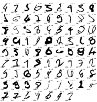
Moreover, there exist different problems in pattern recognition based in the input data and the output expectations. expectations, for example, hand-written digits recognition, as illustrated in Fig. 1.1. Every digit correspond to a 28x28 pixel image. A set of images is labeled by an expert and serves as input to the recognition system. The goal of the problem is tho build a model based on the input data; such that given a new image as input the model is capable of producing a label (0,1, . . . ,9) as output.
Applications such as the example mentioned before, are supervised learning problems because they try to predict labels based on correctly annotated input data pairs, formed by the example and its corresponding label. Rec-ognizing handwritten digits is a example of classification problems, because the goal is to find a label from a finite and discrete set of categorical labels. If the output goal consist in a set of one or more continuous variables, we are talking of regression problems, e.g. having the living areas in m2 and the prices ineof the houses of Barcelona, Catalonia; we would like to know
Figure 1.1: Hand written problem
the prices of other houses in Barcelona as a function of the size of the living areas.
Unsupervised learning is another important field of machine learning, where the goal is to find a hidden structure in unlabeled data. An example is, when the target of a problem is to discover groups inside the input data, based on similarities, this is known as clustering.
Finally, reinforcement learning is the field concerned about how intelligent agents ought to interact with an environment to maximizing some kind of notion of reward. This kind of problems has the target of maximize the reward based in a set of trial and errors.
In supervised learning literature, you will find that each example is a pair of observation and its label. The key idea is to learn a relationship between the observations and their respective labels. Some typical examples are recognizing handwritten digits and email spam classification. Thus, when we have a big volume of input data we start to talk about large-scale systems.
The use of effective machine learning algorithms is really important in in-telligent systems that process large volume of information. Due to the large
volumes of data, conventional supervised learning methods cannot handle such kind of problems, because we cannot store all the data in memory.
1.2
Large-scale learning
We define a learning problem as large-scale, if its training set cannot be stored in a modern computer memory [16]. Furthermore, a deeper definition of large scale learning problem is where the main computational constraint, is the amount of time available rather than the number of examples [6].
An example of these kind of problems is, ad-click data for search engines. When most search engines produce results for a query, they also display a number of (hopefully) relevant ads. When the user clicks on an ad sponsor, the search engine receives some commission from the ad sponsor. This means that to price the ad reasonably, the search company needs to have a good estimate of whether, for a given query, an ad is likely to be clicked or not. One way of to formulate this, as a learning problem is to have training examples consisting of an ad and its corresponding search query, and a label denoting whether or not the ad was clicked. We would like to learn a classifier that tell us given an ad when is likely to be clicked if it were generated for a given query [18].
We call a learning process as online learning when the process is updated one-by-one without re-training using all the learning data when a new learning data becomes available [14].Thereby, online learning has become in the last years an important matter. We would like to address this problem in a specific way, comparing some of the existing algorithms with a new propose made by us.
Kernel based methods have been successfully applied in conventional learn-ing better known as batch settlearn-ing and lastly have been modified to be able to handle online learning. There exist different kinds of online algorithms for example, the kernel perceptron of Freund et al., forgetron method of Dekelet al., subgradient methods [10], etc. Precisely, we focus in this docu-ment on stochastic subgradient descend methods for solving non-separable large-scale problems.
1.3
Approaches to online learning
The batch learning architecture defines that the entire training set has to be available since the beginning of the process. For large data sets this is not a good approach because of memory capacity problems. However the online setting allows the training set to arrive in a stream and like any stream cannot be revisited after it is processed. Some advantages of this approach are:
• It handles very large training sets, because it does not access an ex-ample more than once.
• It adapts to changes in population as time goes on.
1.4
Problems addressed
Online kernel based methods are a very popular method for data modeling and prediction because of their simplicity and good performance on many real-world problems. Many algorithms have been inspired by the Rosenblat perceptron algorithm [11] for finding a separating hyperplane, because is a online learning algorithm for linear classifiers. SVMs are a extension of the original perceptron, incorporating the notion of margin to the learning and prediction process. The kernel trick make SVMs more suitable to work with non-linear data and deal with high dimensional data. The goal of a support vector machines, is to discover the ”most important” training points also called support vectors. Nonetheless, one notable limitation of kernel-based methods is their computational complexity, because the amount of memory that they require to store the support vectors grows linearly with the number of observations, demonstrated in [28]. Thus, for large problems, this number can be large on training and testing. This depend directly of the loss function used but clearly is not satisfactory for genuine online applications.
Typically, the training time grows super linearly with the number of observa-tions. Incremental updates tries to overcome this problem but they cannot ensure a number of updates per iteration. This made them computationally expensive, since they require a matrix multiplication on every update. The methods used here based on kernels exhibit good empirical performance in practice over large-scale scenarios. The most common approach is based on
stochastic gradient descent algorithms which perform perceptron-like up-dates for classification. We have chosen the most popular methods of the state-of-the-art of online learning. However, the performance of online algo-rithms after n observations, is expected to achieved the same as in a batch setting, based in this affirmation for medium-scale problems make sense a comparison with batch algorithms.
1.5
Contributions
In this thesis we present a comparative framework of online kernel based algorithms that deal effectively with addressed problems. They are repre-sentative of the state-of-the-art of online algorithms such us NORMA [26] and PEGASOS [23]. But, it has been previously commented an important limitation of this kind of methods, their computational complexity due to the amount of memory that they require to store the support vectors. There-fore, we devise an online algorithm that improves sparsity property of the actual methods, without losing the generalization ability. To achieve this goal the algorithm proposed employs a deletion process, this can be seen as a revisiting of the support vectors after each update. Making this adjustment, the algorithm allow us to modify standard online proof techniques, so as to provide a bound on the total number of examples the algorithms keeps.
Clearly, our goal is that our method achieves a good reduction in the number of support vectors, while yielding test error rates comparable to the other state-of-the-art online algorithms.
1.6
Layout
This thesis is organized as follows:
Chapter 2 provides background, preliminary theory, notation and formula-tions that are useful when discussing about online kernel-based algorithms.
Chapter 3 present a survey of the state-of-the-art of online learning algo-rithms, describing sub-gradient descend solvers for the optimization prob-lem. NORMA and PEGASOS are explained in detail, their formulation and related approaches.
Chapter 4 introduce the concepts of support vector reduction and the im-plementation of a method denominated SCA for batch settings.
Chapter 5 describe deeply the derivation of the algorithm proposed by us, denominated POLSCA; the formulation and their approaches.
Chapter 6 shows the experimental framework, explaining the methodology followed for the implementation of the algorithms and the analysis of the results.
In chapter 7, we give the general conclusions and personal comments, as well as possible future research work.
Background theory
2.1
Introduction
The main objective of machine learning is the extraction of information from data, from which decisions are made. As we mentioned in Chapter one, we are going to focus on supervised online learning, this chapter has to be seen as a background of concepts, preliminary theory, notation and formulations of the pattern recognition methods.
Supervised learning [18] involves analyzing a given set of labeled observa-tions(the training set) so as to predict the labels of unlabeled future data(the test data). Indeed, the goal is to learn a function that describes the rela-tionship between observation an their labels.
Moreover, in the last years we can observe the growing volume of data, we just have to observe internet where everyday there is more and more information. The online learning approach is necessary in situations where the data arrive in a infinite stream, this is the key idea to use this approach with large-scale data sets. Medium-size problems can be addressed as online learning, providing the data in a streaming way.
Support vector machines are a very popular method used for classification problems inside pattern recognition. They are a subset of a broader number of algorithms known as kernel-based methods.
The classification process involves input data(observation) x and a output decision y. This process can be expressed as in Equation (2.1).
y=f(x) (2.1)
As we are performing binary classification, the pattern recognition algorithm can be considered as a functional mapping of the input data to the output data, if x ∈ Rd and y ∈ {−1,+1} then f : Rd → {−1,+1}. The goal of the pattern recognition algorithms is to determine the value ofyas close as possible to the true value. Given a input data, the classification algorithm will determine the class were the data belongs to, i.e. {−1,+1}.
Some of those kernel methods are the kernel perceptron and a modified version of the perceptron better know as support vector machines. We are going to explain in detail those concepts in the next sections.
2.1.1 Notation
The mathematical notation used throughout this document is described in this section. We represent scalar variables byitalicized lowercase letters and vectors byboldlowercase letters. When we refer to a component of a vector, round bracketing is used. For example,z(i) represents the ith dimension of the vectorz; also can be used the subscripting.
The data used as input for the process is defined in two groups the training set and the test set.
Training set
This set is used for training the algorithms, and find a model that represent the relationship between the observed data and their respective labels. The training set is defined as a set of training examplesS ={(x1, y1), . . . ,(xn, yn)},
where each pair represents:
• xi ∈Rdis a feature vector of dimension d.
Figure 2.1: The Geometrical formulation of SVMs
Test set
The test set is defined as a set of new examples S = (x1, y1), . . .(xn, yn),
that are going to be classified using the model. The new labels ∈ {−1,+1}
are going to be used assess the power of the classification model.
2.2
Support Vector Machines
Support Vector Machines or better called SVMs are a popular method for binary classification, that can be extended to multiclass problems. This method could be seen as an extended version of the perceptron because a perceptron tries to find a hyperplane that separates two classes. SVMs extend this concept trying to find the ”best” hyperplane in the sense of the one that has the maximum margin to the elements of the classes it separates. This definition makes an SVM more reliable, finding an hyperplane that is far away from either classes is considered to be better than any other hyperplane because it generalizes better in front of new data.
In Vapnik et al [8], they follow the idea that an SVM maps the input vector into some high dimensional feature spaceRD, whereD >> dthrough some
non-linear mapping as a RBF kernel; then, in this space a linear decision function is constructed with special properties such that high generalization is ensured.
In order to construct an SVM classifier two problems are to be addressed, one conceptual and one technical. The conceptual problem is how to find a separating hyperplane in a huge dimensional feature space so that it gen-eralizes well; and the technical problem is how to computationally treat such high dimensional spaces. The conceptual problem was solved with the concept of optimal hyperplanes for sepparable cases. Where an optimal hyperplane is defined as the linear decision function with maximal margin between the vectors of two classes. As we observe on figure 2.1, to construct the optimal hyperplane only a small amount of training examples is needed. These examples are called support vectors. This was bound by the concept that if the optimal hyperplane can be constructed by support vectors the generalization ability will be high even in a infinite dimensional space.
Let
wopt·x+bopt= 0 (2.2)
be the optimal hyperplane in feature space. Then, it has been demonstrated that the weights wopt for the optimal hyperplane can be written as some linear combination of n support vectors. This property will be exploited when introducing the kernels and referred as Representer’s theorem.
wopt = n
X
i=1
αixi (2.3)
Then the linear decision function is defined by
f(x) =sign n X i=1 αixi·x+bopt ! (2.4)
Where xi ·x is the dot product between supports xi and the vector x in
feature space.
Nevertheless, even if the conceptual problem has been solved, the technical problem is unsolved. In Vapnik [8] it was shown that instead of making a non-linear transformation of the input vectors followed by dot-products in the feature space; one can first compare two vectors in a input space and
then making a non-linear transformation of the results. This has been solved with the introduction of kernel, for more details see section 2.3.2.
We start the formulation of the SVM by solving the problem of separating non-overlapping classes. This first derivation is also known as hard mar-gin SVM. Afterwards we will relax the non-separable constraint and intro-duce the concept of soft-margin. This allows the treatment of non-separable classes.
Following equation (2.2) that denotes a vectorw commonly referred as the normal of the classification hyperplane and b as a bias. First, we consider the case of a linear separable problem. Thus, there exist a vector w and a bias b such that the equations (2.5) and (2.6) are valid for all the samples in the training set.
w·xi+b≥1 if yi = 1 (2.5) w·xi+b≤ −1 if yi =−1 (2.6)
We rewrite both inequalities as
yi(w·xi+b)≥1, for i= 1,2, . . . , m (2.7)
The distance between the margin and the boundary is 1/kwk, and the dis-tance between margins is 2/kwk as we see in figure 2.1, where w is the unit vectorw/kwk. In the separable case we try to maximize the distance between the margins. Then, the problem can be expressed as
max 2
kwk (2.8)
∀(xi, yi)∈S, yi(w·xi+b)≥1
Equation (2.8) can be easily rewritten as a minimization problem as follows,
min 1
2kwk
2 (2.9)
subject to
yi(w·xi+b)≥1 for i= 1,2, . . . m
Because real data is usually noisy and non-separable without error, then the hard condition has to be relaxed by allowing some examples to be miss-classified minimizing the number of errors. This case is known as the soft margin SVM.
The task now becomes to find a hyperplane with a good trade-off between the training loss and the margin. Also, a large margin leads to good gener-alization of the training set whereas small margins can lead to overfitting. So, we introduce the concept of slack variables, because they soften the hard margin constraints. min 1 2kwk 2+C m X i=1 ξi (2.10) subject to yi(w·xi+b)≥1−ξi ξi≥0 i= 1, . . . , m
The ξi allow the violations of the hard margin constraints, enabling that
some examples lie next to the margin or be missclassified . Moreover, with the addition of the factor P
ξi to the minimization function, we penalize those violations and with C > 0 control the trade-off between the margin size and the amount of slack data.
Support vectors
Up till this point we explained the background theory of SVM, that is a predictor with ”sparse” representation, the so-called support vectors. This vectors influence on the final classification model. Yet, they affect to the computational complexity because they grow up on number with the training examples.
2.2.1 The Primal optimization problem
Most of the books about SVM concentrate in the dual optimization prob-lem [8]. The reader could have the misconception that the dual form is the only way to train a SVM. Primal optimization of linear SVM has been stud-ied in Keerthi and Decoste, and we can find studies about the nonlinear case insub-gradient descend solvers for the optimization problem, their formula-tion and their approaches [7]. As they show, both optimizaformula-tion problems are equivalent. And, when the goal is to find the approximate solution, primal optimization is superior. Based on this affirmations we are going to
optimize the primal formulation of the karnel-based algorithms used on the experimental framework. The primal SVM optimization problem is defined as: min w∈Rd λ 2kwk 2+C n X i=1 ξi (2.11) under constraints yi(w·xi+b)≥1−ξi, ξi ≥0 (2.12)
Rewriting as an unconstrained the SVM optimization problem we obtain:
min w,λ λ 2kwk 2+C n X i=1 `(yi, w·xi+b) (2.13)
where`is a loss function.
2.3
Kernels
The classic formulation of SVM can be generalized considering kernels in a reproducing kernel Hilbert space. Considering non-linear SVMs with a kernel functionk and an associated Reproducing Kernel Hilbert SpaceH.
min f∈H,λ λ 2kfk 2 H + n X i=1 `(yi, f(xi)) (2.14)
Here we can observe the change of variable introducing the regularization parameterλ= 1/C. Because we can control the estimation-approximation trade off by choosingλinstead ofC. We do not use the offsetbfor simplicity.
Kernels-based methods has been successfully used in many batch settings. Researching work in the field of online kernel based methods have been developed, e.g. the kernel perceptron-like updating method by [26], the nonlinear support vector machine solver developed by Shalev-Shwartz et al.[24] or the Relevance vector machine developed by Bishopet al.
In this section we discuss the mathematical framework on which kernel meth-ods are build. First we have some basic definitions:
Definition 1. Kernel, is a continuous function κ:χ×χ→R. A kernel is called positive definite if for any data set{x}N
i=1∈χit satisfies the condition N
X
i,j=1
αiαjκ(xi,xj)≤0,∀αi ∈R (2.15)
Definition 2. Kernel matrix, for a given data set S of N points, theN×N
matrixKwithKij =κ(xi,xj) is called the kernel matrix or Gran matrix of κ with respect to the data set.
2.3.1 Reproducing Kernel Hilbert Spaces
A Reproducing Kernel Hilbert Space (RKHS) is a Hilbert space H with a reproducing kernel whose span is dense in H. LetX be a data set and H be a Hilbert space of functions X. We say that H is a RKHS if for everyx in
X there exist a unique kernel κ(x,·) of H with the followings properties:
1. κ(x,y) =hκ(x,·), κ(·,y)iH wherex,y∈X.
2. The reproducing property,hf, κ(x,·)iH =f(x) wherex∈X, f ∈H.
3. Allf ∈Hare linear combinations of kernel functions. In other words, H is the closure of the span of allκ(x,·) withx∈X.
4. The inner product induces a norm off inH. In other words,kfk2 H =
hf, fiH.
5. Asφ:R→ Rd,φ(·) ={φi}∞i=1 be an orthonormal sequence such that
he closure of its span is equal to H, then,κ(x,y) =P∞
k=1φk(x)φk(y) = φ(x)Tφ(y) if only ifκ is positive definite. Whereφ(·) denotes a map mapping from the input space into a feature space(Mercer’s theorem).
2.3.2 The kernel trick
Until now we have seen how a feature map can be constructed from a kernel. The duality between positive definite kernels and features spaces mentioned in the section 2.3.1 gives rise to the property called the ”kernel trick”: ”Given an algorithm that is formulated in terms of a positive definite kernelκ, one
can construct an alternative algorithm by replacing κ by another positive definite kernelκ0 [4]. This can be directly exploited in the dual formulation of the SVM, for two main reasons [7],
• The duality theory provides a convenient way to deal with the con-straints.
• The dual optimization problem can be written in terms of dot prod-ucts, thereby making it possible to use the kernel functions.
The dual formulation can be expressed in terms of Lagrange multipliersβi
as, max β 1 2 N X i,j=1
yiyjκ(xi, xj)βiβj+
N X j= βj (2.16) subject to N X i=1 βiyi= 0 0≥βi ≤c, i= 1, . . . , N
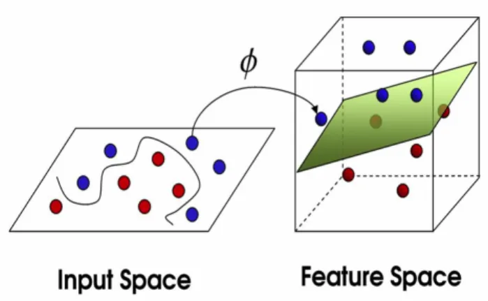
As usually most of the classification problems have high dimensional non-linear features. This property allow us to move on to higher-dimensional spaces, where the features can be linearly separable obtaining a solution that will be a nonlinear function of the input data as we observe on figure 2.2. In other words, if we have an algorithm with a kernel as the inner product in the input space; we can replace that kernel by another(usually nonlinear), obtaining a equivalent performance by the new algorithm.
Though the use of kernels in the dual is straight-forward, they can also be used in the primal, as Chapelle et al. [7] affirm that dual and primal have strong connections. Therefore, they demonstrated that primal and dual optimal values are the same, i.e. that the duality gap is zero. The conclu-sion from their analysis is that even though primal and dual optimization are equivalent, both in terms of the solution and time complexity, when it comes toapproximate solution, primal optimization is superior because it is more focused on minimizing what we are interested in: the primal objective function.
Figure 2.2: Kernel trick
2.3.3 Kernel functions
In this section we describe the most common used kernel functions. As we have seen before the kernel functions represent an inner product in some feature space.
• Polynomial kernel. This kernel is obtained as
κ(x,x0) = (hx,x0i+c)d (2.17)
wherec is a non-negative constant, d∈N is the order of the polyno-mial.
• Linear Kernel. Is a special case of the polynomial with d= 1
κ(x,x0) =hx,x0i=xTx0 (2.18)
• Gaussian kernel. Or Radial basis function(RBF) kernel, is a com-monly used kernel function. It is calculated as
κ(x,x0) =exp −kx−x 0k2 2σ2 (2.19)
Whereσ >0, is a scaling constant . This is the most popular function in used in the optimization problem of support vector machines.
The RBF kernel spans an infinite dimensional space. However, this does not suppose a computational problem, because the kernel trick allow us to perform the scalar product between two points in the infinite-dimensional space by calculating the kernel function of the data in the input space.
2.4
Loss function
The loss function is a measure of empirical error, where the error is generated by the training process. Parameter estimation for online kernel learning task as classification can be formulated as a loss function over a training set.The loss function quantifies the amount by which the prediction deviates from the actual values. Indeed, an ideal loss function has the following properties.
• It has to be convex for easy optimization, that means that has a unique optimum and that if we drawn a line between two points of the func-tion, this line does not cross the function.
• It is robust, it copes with outliers.
• It gives sparse solutions, in the primal domain that means that all the features are not needed to specify the decision boundary; in the dual domain means that not all samples are required to specify the optimal solution.
There exist different loss function types, some of them are explained here.
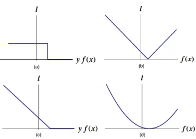
2.4.1 0-1 loss
As we observe on the figure 2.3, the 0-1 loss function does not penalize if the data point is correct labeled, but if not gives a penalization value of 1, always.
`(y, f(x)) = (y =6 f(x))0−1 (2.20)
It is not convex, is robust because the error doesn’t grows. It is sparse but has an ambiguous optimum.
2.4.2 Absolute loss
It is described as follows:
`(y, f(x)) =|y−f(x)| (2.21)
Absolute loss function is applicable to regression problems just like square loss, and it avoids the problem of weighting outliers too strongly by scaling the loss only linearly instead of quadratic by the error amount.
2.4.3 Hinge loss
The hinge loss function is illustrated in figure xx and formulate by equation (2.22).
`(y, f(x)) =max(0,1−yf(x)) (2.22)
It works well for the purposes in SVMs as a classifier, since the more you violate the margin, the higher the penalty is. However, hinge loss is not well-suited for regression-based problems as a result of its one-sided error. Luckily, various other loss functions are more suitable for regression. More-over, it is sparse, because specifies the classifier in terms of small faction of the training set.
2.4.4 Square loss
Square loss is one such function that is well-suited for the purpose of regres-sion problems. Is formulated as follows:
`(y, f(x)) = (y−f(x))2 (2.23)
However, it suffers from one critical flaw: outliers in the data (isolated points that are far from the desired target function) are punished very heavily by the squaring of the error. As a result, data must be filtered for outliers first, or else the fit from this loss function may not be desirable.
Online learning
3.1
Introduction
This chapter will introduce three existing approaches to solving the primal formulation optimization problem. First, we formulate the perceptron and extend to kernel-perceptron and SVMs methods. The state-of-the-art in Online learning has a bunch of solvers, we would like to focus on stochastic subgradient descend solvers for the regularized Hinge loss formulation of the Risk minimization and the soft margin SVMs. For construct the comparative framework we have selected two algorithms that present a good performance, and we will propose a new one.
Subgradient based methods have the advantage of being significantly sim-pler than other methods. We introduce some important concepts before the introduction of the algorithms. Then, we present the implementation pro-cedures of the algorithms PEGASOS and NORMA, and the theory behind them.
3.2
Perceptron
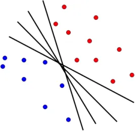
Rosenblatt’s perceptron algorithm [11] is the first and most simple algorithm for online machine learning. The training procedure says that a perceptron has associated a weightvector w= [w1, w2, . . . wd]. Each perceptron has a
Figure 3.1: The perceptron divide the space using an hyperplane thresholdθ. The output is +1 if w·x > θ −1, ifw·x < θ
The special case ofw·x=θwill always be regarded as “wrong”. This case helps to defines a hyperplane of dimensiond−1 as in the figure 3.1.
Some problems or limitations of the perceptrons are:
• Sometimes the data is not separable by an hyperplane.
• Classes can be separable by more than one hyperplane and not all of them are equally good.
• Most rules for training a perceptron stop as soon as there are no miss-classified points. As a result, the chosen hyperplane will have a poor generalization of unseen data.
The perceptron algorithm can be extended to use kernels, in this setting we are dealing with kernel perceptron algorithms as NORMA [26] or ALMA [12]. This extension allow them to manage some of the limitations that they have, now they can deal with data set non-linearly separable. NORMA is a good
example of this kind of algorithms, we are going to formulate, analyze and implement it.
3.3
Stochastic sub-gradient descend method
This method, iteratively search for the optimum of a function. It starts with a random point, finds the best search direction, computes the new point and repeats these steps until it converges.
In the previous chapter, we defined how is formulated the minimization problems for classification. Gradient based methods works well with large scale classification and regression problems of high dimension feature space, making it suitable for our goal.
The method of gradient descent is based on the concept of the gradient. The gradient of a function∇Φ at a point defines the direction along which the function grows faster. If we defined the optimization as a function Φ(w), then −∇Φ points to the greatest decrease; so, the equation (3.1) describe the update an estimatedwt that in a iterative scenario finds the minima of
Φ.
wt+1=wt−ηt∇Φ(wt) (3.1)
Where, ηt is the learning rate, which determine how far we move in the
direction of the gradient. This is a important parameter because, if its too small the convergence is slow, and if it is too large then we can overshoot and miss the minimum.
Stochastic gradient descend unlike gradient descent that uses all the entire training set to compute the gradient, find the gradient with respect to a single randomly chosen sample. This is suitable for online scenarios for two important reasons; its significantly quicker than gradient descent for large data sets, and it minimizes the generalization error quicker than gradient descent.
wt+1=wt−ηt∇Φi(t)(wt) (3.2)
Where i(t) is an index choose randomly from (1,2, . . . k). With a single example we are obtaining an approximation to the true gradient; therefore, we are not longer guaranteed to move in the direction of the greatest descent.
Gradient descent and stochastic gradient descent assume that Φ is a differ-entiable function of w, then ∇Φ is always well defined. Besides, if we wish to solve the optimization problem described in (2.14), this assumes that `
and the regularization termr are differentiable, which does not always hold. As ` and r are convex functions, even if they are not differentiable, they can be lower bounded at any point by asubgradient. The subgradient∂(w) consist of all vectors that are lower bounds to the function atw.
∂Φ(w) ={v∈Rd: (∀w0)f(w0)≥f(w) +v·(w0−w)} (3.3)
The update equation of the stochastic gradient descent becomes:
wt+1 =wt−ηt k
X
i=1
∂Φi(t)(wt) (3.4)
3.4
Kernel machine algorithms
We have seen the theory of kernel machines in the former chapter. Now we are going to derive some of the most popular kernel machine methods, that uses stochastic subgradient descent to solve the optimization problem.
3.4.1 NORMA
The Naive Online Risk Minimization Algorithm by Kivinen et al. [26] has introduced as a efficient method for classification, novelty detection and regression using stochastic subgradient descent with respect to an instanta-neous risk function as en equation (3.8). The goal is tho find a function f, such as describe a relationship between the observations and their labels. In batch learning, it is usually assumed that the data are drawn independently from some distributionP overX xY. Moreover, the generalized loss func-tion is described as `{x, y, f(x)}, and the expected risk of the function f is defined in equation (3.5) as a measure of quality off.
R[f, P] :=E(x,y)∼P[`(x, y, f(x))] (3.5)
instead of equation (3.5), collected k observation and label pairs. Remp[f] := 1 k k X t=1 (`(x, y, f(x))) (3.6)
However, minimizing equation (3.6) could lead to overfitting; normally occur when complex functions model the training data but do not generalize well new data, that means that have poor predictive power. One way of avoid this is introduce a penalization to complex function, then instead of minimize the empirical risk we are going to minimize the regularized risk (3.7).
Rreg[f] :=Rreg,λ[f] :=Rreg[f] +λ 2kfk
2
H (3.7)
Where λ > 0 allows the amount of complexity been chosen appropriately for each problem, and kfk2
H measure the complexity in a possible infinite
dimensional Reproducing Kernel Hilbert Space(RKHS). Therefore, as we are interested in online algorithms, where you get one-by-one example; we define a instantaneous approximation ofRreg,λ, the instantaneous regularized risk on a single example(x, y) is formulated as
Rinst[f,x, y] :=Rinst,λ[f,x, y] :=Rreg,λ[f,(x, y)] (3.8) NORMA is a stochastic gradient descend method perform respect to the instantaneous risk. The general idea of the update is expressed as,
ft+1 ←ft−ηt
∂(Rinst[f])
∂f (3.9)
Kivinen suggest that the value of the learning rate ηt has to bigger than
zero and often constantηt=η.-Its value is going to be adapted using cross-validation, because offer great results but is a computationally expensive. There no exist a lot of literature about this subject, Vishwanathanet al.[21] suggest an algorithm referred as Stochastic Meta-Descend (SMD) but re-quires more computational effort.
ft+1 :=ft−η∂fRinst,λ[f, xt, yt]f=ft, fi∈H (3.10) ft+1 :=ft−η∂f λ 2 kfk 2 H + 1 n n X i=1 `(f(xi), yi) ! ft+1 :=ft−η λ 2∂fkfk 2 H + 1 n∂f n X i=1 `(f(xi), yi) !
Like we are treating one example by one example, we can eliminate theP
of the loss function and his coefficient:
ft+1=ft−η∂f λ 2kfk 2 H +`(f(xi), yi)
in order to evaluate the gradient, note that the evaluation functional f 7→
f(xi) is given by the reproducing property in RKHS:
hf, k(x,·)ih =f(x) for x∈X
and therefore
∂f`(f(xt), yt) =`0(f(xt), yt)k(xt,·)
Since∂fkfk2H = 2f based on the affirmation in [26], the update becomes:
ft+1=ft−ληft−η`0(f(xt), yt)k(xt,·)) (3.11) ft+1= (1−λη)ft−η`0(f(xt), yt)k(xt,·))
By the representer theorem we can express as
t−1 X i=1 αik(xi,·) +αtk(xt,·) = (1−ηλ) t−1 X i=1 αik(xi,·)−η`0(f(xt), yt)k(xt,·)
Then we obtain finally:
αi = (1−ηλ)αi for i < t (3.12)
αt=−η`0(f(xt), yt) for i=t (3.13)
The loss function used for the classification problem is the Hinge Loss that satisfied the formulation (2.22). Then equation (3.13) become
αt=ηyt1[ytft(xt)−1≤0] (3.14)
Data: (xi, yi)∈S Result: Model initialize; Buffer, SV = 0; m= 0, f0= 0; while t < τ do
At time t, take sample and label pair (xt, yt) ;
if ytft(x)≤ρ m=m+ 1; α(m)←ηyt; StorextinSV; fori←1. . . m−1 do α{i} ← {1−ηλ} α(i); end Discardxt, yt; end
Algorithm 1:Naive Online Risk Minimization Algorithm
Speedups and truncation
There are several ways of speeding up the algorithm proposed by Kivinen
et al. Instead of updating all old coefficientsαi, i= 1,2, . . . , t−1, one could simply cache the power series 1,(1−λη),(1−λη)2, . . .. A mayor problem with (3.12) and (3.13) is that the kernel expansion at time t contains t
terms. As the computational complexity grows linearly with the size of the expansion. The regularization parameter helps here, because after τ
iteration the coefficients αi will be reduced to (1−λη)ταi.Hence, we can
drop small terms and incur in a little error. This methods are going to be applied in the implementation time, dropping all the terms that have a weight <1e−8.
3.4.2 PEGASOS
In this section we describe the primal estimated sub-gradient solver better known as PEGASOS, for solving the optimization problem given by the equation (2.14).
It is closely related with NORMA, because both are based on SGD methods, but PEGASOS augment a subgradient projection. The algorithm uses a
subset of k training examples, where k is supplied by the user and represent the size of the minibatch on the training data. The algorithms proceed as follows: at each iteration, a random subset of k training examples is chosen; then it computes a approximate subgradient function evaluated on these k examples, updating the weight vector values. Subsequently, the vector is projected onto a L2 ball of radius 1/
√
λ. This is made because it can be proven that the optimal solution always lies inside this ball [23], projecting it brings it only closer to the optimal solution.
The general idea is that the method starts with a random starting point, finds the best search direction, computes the new point and repeats until it converges. An important property about PEGASOS [18], is that it con-verges to theρ-approximate solution in ˜O(d/λρ) iterations, where d is the maximum number of non-zero features in each example. This differ from theO{1/ρ2} convergence of NORMA.
When k=1, PEGASOS is just a SGD method with a projection step, that make it very similar to NORMA. More exactly, there is a couple of important distinctions. First,after each gradient-based update, the learning rate is decayed by ηt = 1/λt, when λ is the regularization parameter. Second, the projection of the weight vector involves that kwk ≤ 1/√λ; this step, ensures a feasible and very aggressive decrease in the learning rate, in that still possible to bound the number of iterations by O(1/ρ).
Nevertheless, when k=m it is nothing but a sub-gradient projection this present it as a gradient descend algorithm with a improved convergence rate.
The algorithm perform two-step update as follows. First, we scale xt by
(1−ηtλ) and for all the examples that belongs to the minibatch we add
thexthe vector yηt
k x. They denote the vectorwt+12. This step can also be
written as wt+1 2 =wt −ηt∇t where ∇t=λwt− 1 k k X i=1 yx
Last, we set wt+1 as a projection ofwt+1
2 on to the set
B={w:kwk ≤1/√λ} (3.15)
Indeed,wt+1 is obtaining by scalingw1/2 by min{1,1/(
√
λkwt+1 2
k) as they show the optimal solution is in the setB. In other words, we are projecting onto the setB as we only get closer to the optimum.
As we are using the single randomly selected example case and not the minibatch setting, the algorithm stays as is described on algorithm 2.
Data: (xi, yi)∈S Result: Model initialize; DatasetS; τ,λ; b←0; fort←1,2, . . . τ do
Pick a random example xi, yi; Setηt←1/(λt); if yifi(xi)≤1 α←(1−ηtλ)α+ηtyixi; b←b+ηtyi; else α←(1−ηtλ)α; end
Algorithm 2:Primal Estimated sub-GrAdient SOlver
Convergence of pegasos
Due to the aggresive decay of the learning rate, the probability of converge and the computational time required by the algorithm make it successfully in the last few years.
Support Vector Reduction
4.1
Introduction
The algorithms presented until now, are kernel-based solvers on optimization problems. Their goal is to seek a relative complex function that maximizes the margin, modeling the training data without overfitting them. A very important parameter is the number of support vectors. As we mention previously this parameter bounds the computational and memory efficiency, because they determine the expansion of the kernel machine [8].
Due to the kernel trick, we can now work in huge dimensional feature spaces without having to perform calculations explicitly in this space as we men-tioned in chapter 2. Hence, the representer theorem introduced by Kimel-dorf and Wahba, implies that the number of support vectors grow up linearly with the number of the training examples in the training set demonstrated in [28].
Besides, we have to scale the problems described above to an online scenario, where the training data is see it as a infinity stream. The time complexity required to perform kernel machine algorithms grows linearly with time, in this scheme can be seen that grows without bound. Then, is necessary to explore some methods that allow us reduce the number of support vectors.
Several methods have been proposed to help the number of support vectors, Tran et al. apply clustering techniques to reduce support vectors, Argawal
et al.[27] present us a technique based on span distances. Downset al.[29] present an algorithm that eliminates support vectors linearly dependent on the other support vectors.
The separable case approximation proposed by Geebelen et al. [9] propose that made the training set separable, by first removing missclasified exam-ples or by swapping their labels, and then, solve the problem with that mod-ified training data. This algorithm is closely related with Bottou [6] work based on cross-training technique; where they first, categorize the training samples depending on their weights, train a SVM for every subset and com-bine the results in a model, breaking the linear dependency between the number of support vectors and the training samples.
4.2
Separable case approximation
In Geebelen et al. is discussed that the separable case approximation al-gorithm (SCA), improves the sparsity of SVM classifiers. The goal of the sparse approximation problem is to approximate the SVM classifier defined by w and b by a sparse SVM classifier defined by w0 and b0, such as the approximate classification model has the performance as similar as possible to the original model.
We define ˆy(x) and ˆy0(x), as the label of a observation according with the original and the approximating classifier respectively. SCA propose to mod-ify the training set by flipping or removing the missclasified examples. Then the approximation problem becomes a classification problem over a modified training set. In both cases, the modified training set is separable because the non-pruned solution separates it. This separability only holds when the SVM classifier used to solve the approximation has the same kernel as the original classifier. They exploit this separability to gain sparsity. The algorithm 3 describes SCA deeply.
Data: (xi, yi)∈S
Result: SVM-solution for the separable case Given a SVM model solutionf(x);
forj←1 to nSV do if yf(x)≤0
Flip the label ofxj,yj=−yj; or;
Discardxj,S0=S− {xj};
end
Given S0, findf0(x);
Algorithm 3:SCA algorithm
The final support vectors lies close to the original separating hyperplane. It is demonstrated that the SVM classifier for the separable case, will generally not find more support vectors than d+1, where d is the dimensionality of the feature space. This algorithm present a upper bound, due to all support vectors lie on one of two parallel hyperplanes in the feature space. Moreover, the degrees of freedom for choosing two parallel hyperplanes in a d-dimensional space is equals to d+1. If exist circumstances as linear dependency between p or less training data points, this upper bound can be exceeded.
In the practical work of Geebelen, it is described that the number of support vectors reduces drastically; the support vectors of the pruned solutions lie close to the decision boundary of the non-pruned solution, then the training set accuracy does not decrease after the pruning, as expected. This work has been developed under the batch learning scheme.
POLSCA
5.1
Introduction
After explained some of the most used kernel machine solvers for classifica-tion and their drawbacks, we would like to propose a new algorithm that solves the problems addressed by online learning and improves the sparsity of other methods as PEGASOS or NORMA.
Our idea is improve the performance of PEGASOS trying to reduce the number of support vectors, dealing in this way with the computational com-plexity addressed problem. At the same time we require that our proposed algorithm do not afford a loss in accuracy. This means that the accuracy has to be close to PEGASOS or NORMA, as minimum. Then, our proposed approach is an algorithm that improves the performance of PEGASOS by applying SCA in some way that allow us to reduce the number of support vectors with minimum loss in accuracy.
Another issue is the computational time cost, we are not allowed to take more time than NORMA as minimum, because is demonstrated in former chapters that PEGASOS is faster than NORMA. Then, once we have de-fined our goals and requirements, we propose a method denominated Primal Online Sub-gradient Algorithm (POLSCA).
5.2
Primal OnLine Sub-gradient Case
Approxima-tion Algorithm
The algorithm proposed here tries to overcome the sparsity of the algorithms described in former chapters. Our proposal starts with the analysis of four categories of samples found on the SVM optimization problem, we have categorized them as,
• Subset A: 1−ε ≤ yif(x) = 1 +ε, are the ordinary support vectors
because they lie next to or in the margins hyperplanes, whereεallow a relaxation tolerance on the margin conditions to classify points.
• Subset B: ε≤ yif(x) ≤ 1−ε, examples that lies in this interval are denominated margin errors because they include the vectors between the decision boundary and the margins that are well classified.
• Subset C:yif(x)<0 , are the missclassified examples, in soft margin svm this are allowed and affect to the decision boundary.
• Subset D: yif(x) > 1 +ε, are the well classified examples that does
not play any role on the optimization problem. Their deletion will not affect the model.
The key idea of POLSCA is to merge the idea behind SCA inside the online learnig process of PEGASOS, so we are going to based on the PEGASOS al-gorithm as starting point. Then our initial alal-gorithm proposition is detailed in 4.
Data: S, τ, SV, α, b
Result: SVM-model approximate solution ˆfibased on SV, α, b
fort←1 toτ do
Pick a random example xi, yi;
if yf(x)≤1then updateSV, α, b; else updateα; end end
CheckSV subset for deletion;
forj←1 to nSV do
Choose a xj, yj;
if yf(xj)< threshold then
Delete selectedxj from SV, wherej= 0, . . . , z;
end end
Algorithm 4:General algorithm proposed
Initially the threshold was set to zero as SCA proposed, but this was observe as an aggressive deletion step. At the beginning the algorithm is away to converge. Then, we looked for a threshold value that allow us not so aggressive behavior. So, we proposed a ς threshold value that allow us to relax the deletion step. This value proceed in a progressive updating with the iterations.
The updating of theςis controlled for another variable denoted asϕ. Indeed, we cannot delete all the support vectors that satisfied the threshold condition of the deletion step, because could give us the case that all the support vectors are deleted. So, to avoid this problem we add a controlling step that let us keep a minimum number of support vectors.
Accordingly, after each update step of POLSCA, we are going to verify the belonging of the support vectors to the above defined subsets. The deletion step will start with a smooth condition allowing to eliminate random vectors from the support vectors founded until the moment.
yif(x)< ς (5.1)
where ς =min e1−eϕ/t,0, and ϕ can have the value of (τ, τ /2, τ /3, . . .) depending on the speed that we want to bound the support vectors to the subset A and B. The key idea is to arrive after some number of iterations
to the condition where missclassified examples are not allowed.
This deletion condition that tends to eliminate missclassified examples, will improve the sparsity of the algorithm against NORMA and PEGASOS. The algorith is detailed in Algorithm 5. Based on the optimization problem, we define the update-step for POLSCA based on
wt+1=wt−ηt∂f λ 2wt− 1 k k X i=1 yκ !
An the alpha vector is update as follows
α= (1−ηtλ)α+ηtyiκ(x,·) (5.2) Data: (xi, yi)∈S Result: Model Initialize; DatasetS; Buffer, SV = 0; τ,λ, ϕ; b←0; fort←1,2, . . . τ do
Pick a random example xi, yi;
ηt←1/(λt); ς =min e1−eϕt,0; if yifi(xi)<1 α←(1−ηtλ)α+ηtyiκ(x,·); b←b+ηtyi; StorextinSV; else α←(1−ηtλ)α; forj ←1,2, . . . mdo
Choose a support vector samplexj, yj fromSV;
if yjfj(xi)< ς andm > minimum deletexj, yj fromSV;
end end
Algorithm 5:Primal Online Sub-gradient Case Approximation
Experiments and results
6.1
Introduction
In this section the protocol, databases, performance measurements and pa-rameter settings are described alongside the experiments conducted and re-sults achieved.
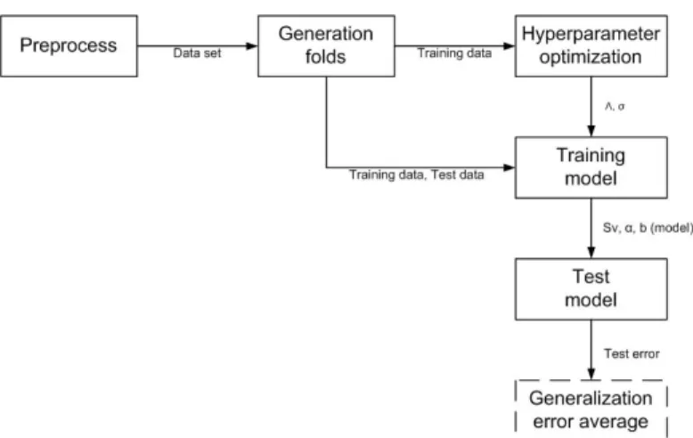
The experiments were conduced, first on baseline experiment with a toy data set. Then, with high dimensional features space using popular medium-scale databases from UCI [2]. In each step, were followed the protocol illustrated on figure 6.1 and were verified the ability of POLSCA, our proposed algo-rithm in front of PEGASOS and NORMA. All of them alongside with a batch solver for medium problems implemented using CVX package soft-ware, to track the generalization error of every algorithm.
All experiments usually follow a protocol, proposed by the author. In this thesis will not be in a different way.
Fist of all, we are going to divide the experiments as
• Baseline experiment.
• UCI experiments.
• Quasi-large scale experiments.
6.2
Databases
Our baseline experiment is based on a toy problem described on table 6.1. It is a synthetic database formed by two normal distribution of data points, with a medium of 5 and 10; and a variance of 2 and 2.5 respectively. It is a 2-dimensional problem, making easy to illustrate the behavior of POLSCA in front of other algorithms. The data set is composed of 500 samples distributed in two classes of 250 each one, represented an ideal balanced problem.
Database Examples Features
Toy problem 500 2
Table 6.1: Toy data set
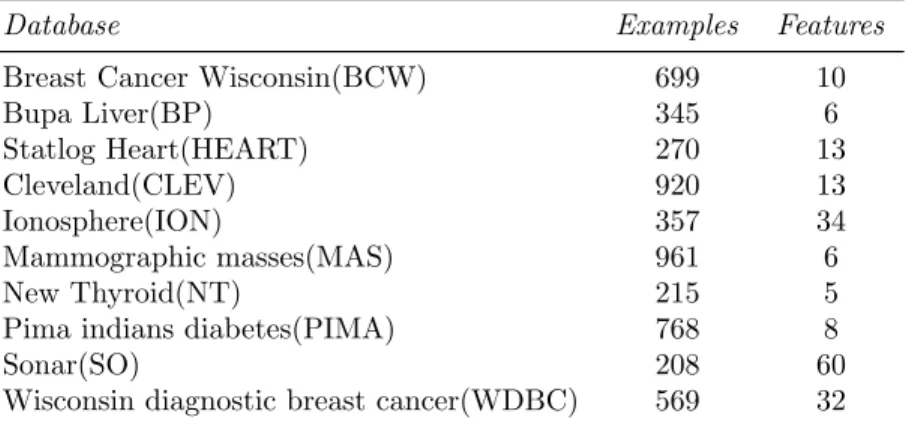
The next table 6.2, describes the selected medium-scale data sets used for the denominated UCI experiments, some of them are multiclass problem, then we are going to use the one-against-all policy, because we are going to work with binary classifiers. These data sets can be downloaded from the UCI website [2].
Database Examples Features
Breast Cancer Wisconsin(BCW) 699 10
Bupa Liver(BP) 345 6 Statlog Heart(HEART) 270 13 Cleveland(CLEV) 920 13 Ionosphere(ION) 357 34 Mammographic masses(MAS) 961 6 New Thyroid(NT) 215 5
Pima indians diabetes(PIMA) 768 8
Sonar(SO) 208 60
Wisconsin diagnostic breast cancer(WDBC) 569 32
Table 6.2: UCI databases
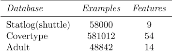
Finally, the quasi-large scale experiments are selected from UCI large-scale data sets. We have choose three data sets for the comparative framework as we observe in 6.3.
Database Examples Features Statlog(shuttle) 58000 9 Covertype 581012 54
Adult 48842 14
Table 6.3: UCI quasi-large scale databases
All the databases has been preprocessed before use them, detecting missing values and replacing them by the average value of that feature. Then dis-cretizing the categorical and continuous features. Next, choosing a policy for instance selection that in our case will be random selection. Finally, for this experimental framework we are going to used a very common method based on equation (6.1) to Normalize the data set.
v0= v−v
maxv−minv
(6.1)
wherev is the old feature,v0 is the new one andv is the mean of vectorv.
6.3
Performance measures
Performance measures quantitatively tell us something important about the behavior of POLSCA and the methodology that process them. They are a tool to help us understand, manage, and improve our proposed algorithm.
Consequently, the methodology that our comparative process follow in gen-eral lines is:
• Pre-process the data.
• Select the kernel to use.
• Select the best hyperparameters (cross-validation with grid search).
• Train the model with the best hyperparameters and test (using cross-validation).
Figure 6.1: Flow chart of the methodology.
The efficiency of POLSCA will be determined by the number of support vectors, the accuracy and the time complexity. The accuracy particularly is going to be measured making a comparative with the baseline model for the baseline and medium-scale experiments. The baseline model is based on a batch optimization implementation using a software package denominated CVX. All of the implementations are made over the MATLAB framework.
6.3.1 Baseline model: CVX optimization
Since the optimization problem described former is convex, then it can be optimized using a standard convex optimization package as CVX [1]. Many convex optimization problems can be solved by several off-the-shell software packages including CVX, Sedumi, CPLEX, MOSEK, etc. This allow you, once you identify the convex optimization problem, you can solve it without implement the algorithm yourself.
This has been selected as a baseline, as CVX works in a batch setting, we cannot use it with large-scale databases.
CVX is a free MATLAB-based software package for solving generic convex optimzation problems; it can solve a wide variety of convex optimization problems such as LP, QP, QCQP, SDP, etc. Indeed, the binary optimization problem using non-linear kernels is going to be implemented on this package.
6.4
Parameters setting
The parameter setting scheme, needs that initially we choose a kernel for the implementation of the algorithms, we are going to select the same for all the algorithms in this way we are making more balanced the comparative scenario.
6.4.1 Kernel selection
One of the important advantages of using SVMs or kernel perceptrons meth-ods, as we have seen on Chapter 3, is their ability to incorporate and con-struct non-linear predictors using kernels thanks to the kernel trick.
As we are working with non-linear and high dimensional problems, we choose the Radial Basis Function kernel. Therefore, is a standard and very popular kernel, so we have decided for this after try others, because their approach is helpful for the experimental framework.
The kernel parameterσtogether with the regularization parameterλare de-nominated hyperparameters. The optimization of them achieves two steps, first we have to define the interval for the grid search. Once this has done we have to realize a training and test process based on cross validation to select the best hyperparameters. This process is made over the training set.
6.4.2 Grid search
Hyperparameter optimization is an important matter, with this we ensure that the model is not over-fitting the data. As we do not know the best values for hyperparameters we can based on different criteria like random search, grid search or heuristic based methods to find them.
We use grid search because is an exhaustive hyperparameter search, even if the computational time is more than others, it offers the security that we are looking all the space of possible values ofλandσ. Specifying the hyper-parameter space interval where grid search is going to be build. The grid search is going to be constructed over exponentially sequences. Therefore, the interval for λvalue with good performance is found inside the interval (10−5,10−4...105), andσ in (2−5,2−4, . . . ,25).
Hence, once we have defined the interval for values ofλandσ, then we have to use 5-fold-cross-validation to find the best hyperparameters. The best pair is that one presenting the best average accuracy after cross-validation in the training set.
6.4.3 Cross Validation
We use k-fold-cross-validation in the training set to find the best hyperpa-rameters. The literature about this says that we have to divide the set in k-folds, one set is going to be use to test and the others to train. Using grid search and cross-validation we are able to find the best hyperparameters in the grid search space for ours 4 algorithms(CVX, NORMA, PEGASOS and POLSCA).
It is found that more than one pair of parameters works well, then we decided to pick up the first one. Once the cross-validation step for hyperparameter optimization is done, the next step is to take them them and train a model ant test it to obtain the generalization error. Thereupon, we do 10-fold to obtain a average generalization error that allow us to obtain a average accuracy of every algorithm.
6.4.4 Training and Test
Subsequently, after the hyperparameter optimization step for NORMA, PE-GASOS, and POLSCA; with the results we should train a model for the different algorithms. Therefore, once the best hyper-parameters are chosen. The next step is to train the models, the most common technique is k-fold cross-validation, we use it to find the generalization error of every model.
Once we have the generalization error of the models we can compare those results with the baseline algorithm and between them. We start with the toy experiment following with the medium-scale and finally the large-scale UCI experiments.
6.5
Results
Here, we are going to describe the results obtained after the implementations following the methodology for processing input data. In our experiments we compare CVX, NORMA, PEGASOS y POLSCA using the datasets provided in the section 6.2.
6.5.1 Baseline experiment
As we said before, the baseline experiment is a balanced problem with quasi-ideal conditions, that help to measure the performance using the described in section 6.3. Therefore, is very useful as an illustrative base case to observe the performance of the algorithms and compare their behavior.
CVX NORMA PEGASOS POLSCA
SV Acc(%) SV Acc(%) SV Acc(%) SV Acc(%) Toy 450 94.60 1350 93.60 307.4 94.60 290.4 94.40
Table 6.4: Number of support vectors and accuracy
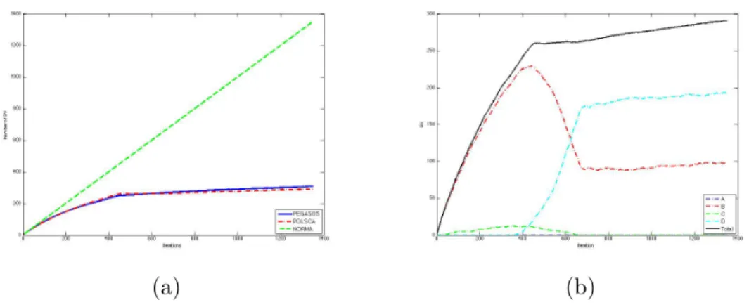
We have defined theτ equal of ten times the size of the data set to observe if the performance improve with iterations. As we observe in the figure 6.4 after the 400th iteration POLSCA starts to reduce the support vectors in comparison with PEGASOS and NORMA has a linear behavior.
Therefore, we are dealing with a medium size data set and present a re-duction around of 8% of the support vectors and a loss on accuracy about 0.2%. Accordingly with the expectations this means that POLSCA has a good behavior and we can continue to the next experiments. Accordingly, the requirements were fulfilled, because POLSCA present a reduction of support vectors with respect to the state-of-the-arts methods as NORMA or PEGASOS.
Figure 6.4, in (a) shows the behavior of the different algorithms, with a similar tendency. In b, we observe different subsets that affect the total number of support vectors in POLSCA, the more representative subset is B, that are the support vectors that lies between the margin and the boundary of the model. Moreover, this allow us to explain the POLSCA approach,
(a) (b)
Figure 6.2: (a) SV distribution for algorithms, (b) SV subset distribution for POLSCA
eliminating missclassfied examples without losing accuracy respect to PE-GASOS or even CVX. Then, we observe that after some iterations the subset C disappear.
Figure 6.3: Deviation of SV
Figure 6.3, shows how POLSCA present an improvement than PEGASOS relate to the deviation of the number of support vector with the iterations. As the deviation represents how much variate or scatter is the data related to their mean, POLSCA present a ”better” behavior related to PEGASOS.
be-(a) (b)
(c) (d)
Figure 6.4: Comparative between the different algorithms for every subset
cause involve the support vectors that are on the margin. We can observe how the subset B for POLSCA starts to decrease after some iterations, but PEGASOS continue increasing with moderate behavior.
Moreover, the subset C once are detected all the misclassified examples in POLSCA they are deleted, with PEGASOS they remains constant. Still up now, NORMA increases the number of support vectors in all subsets due to we do not apply any truncation method.
The accuracy of the algorithms for this case are similar, specially after some iterations. We can derive the comment that PEGASOS and POLSCA need a certain number of iterations to calibrate; in the figure 6.4 we see that POLSCA is more constant once has passed this calibrated phase.
6.5.2 UCI medium-scale experiments
Our second experiment involves real UCI medium-scale data sets, all the experiments were carried out by splitting the data sets in subsets due to the use of cross-validation. Indeed in table 6.5, we have the final average accuracy results after the cross validation.
CVX NORMA PEGASOS POLSCA
SV Acc(%) SV Acc(%) SV Acc(%) SV Acc(%) BCW 342 97.20 3150 95.80 36 96.38 33 96.81 BP 308 70.60 1540 58.79 157.4 60.31 103.7 59.09 HEART 243 84.07 1215 77.04 177.6 77.04 176.2 77.09 CLEV 829 74.40 4145 72.89 313.78 73.75 286 73.38 ION 317 91.66 1585 85.00 225.7 83.24 186.2 82.94 MAS 842 83.67 4330 81.89 73.2 81.50 56.1 81.26 NT 194 93.34 970 91.00 108.7 93.00 108.5 92.38 PIMA 692 77.63 3460 74.87 481.1 75.79 314.7 74.08 SO 183 90.80 940 86.00 177.8 83.00 184.3 85.50 WDBC 513 98.40 2565 96.25 460 96.42 406.5 95.89
Table 6.5: Number of support vectors and accuracy results to medium scale experiments
Table 6.5 gives a general vision about the behavior of POLSCA, over differ-ent data sets, after this results we can affirm that POLSCA has a confiddiffer-ent behavior, in 9 of 10 experiments the requirements are fulfilled related to the number of support vectors. One of them reports the best behavior of POLSCA, this happen with thePimadata set where the number of support vectors is reduced about a 35% with respect to PEGASOS and the accuracy is reduced by 1.7%. The accuracy in those cases is closed to the PEGASOS values. In the only case that this does not happen and POLSCA present an average number of support vectors larger than PEGASOS the accuracy is better.
The figures from 6.5 illustrated the most representative data set from table 6.5. The behavior allow us to continue with quasi-large scale experiments with confident. Due that POLSCA is going to be tried in the most demon-strative scenario, with large-scale data sets.
(a) (b)
(c) (d)
Figure 6.5: Support vector vs. Iterations of the most representative UCI data sets
6.5.3 Quasi-Large scale experiments
Finally, we apply our algorithm to large scale problems. The UCI Statlog Shuttle dataset, the Cover Type and the Adult data sets are the selected ones for the experiments. They have more than 45000 examples that made them suitable for try our proposed algorithm. In this phase, CVX is not implemented anymore because the computational cost is too huge for the RAM memory, made them infeasible to compute.
NORMA PEGASOS POLSCA SV Acc(%) SV Acc(%) SV Acc(%) SHUTTLE 34801 98.03 594.4 93.86 460.2 97.21 COVER TYPE 96809 72.28 9039.6 70.37 7152.4 70.39 ADULT 48534 81.19 10578.4 81.32 6909.2 80.38
Table 6.6: Number of support vectors and accuracy for large-scale data sets
Table 6.6 present the results of the experiments, we can generalize that POLSCA in online scenarios has a good trade-off between accuracy and the number of support vectors; this can be observe over the larger experiment were POLSCA obtain a reduction of 20.9% without any loss instead a 0.02% of improvement related with PEGASOS and a loss around 2% approximately against NORMA. The computational time increase due to the grid search for hyperparameter optimization, to reduce the cost of this stage we have decided to use just the 70% of every data set respectively.
(a) (b)
Figure 6.6: Quasi Large scale experiment results where (a) and (b) refers to Shuttle database results, (a) the number of support vector of PEGASOS in the left and POLSCA in the right, and (b) The accuracy starting with NORMA, in the middle PEGASOS and in the right side POLSCA.
Figures 6.6 shows in (a) and (b) how POLSCA has an approximate reduction about the 35% in the Statlog Shuttle data set. Therefore, with Cover Type POLSCA present a reduction of 22,5% with a loss in accuracy of 0.02% illustrated in figure 6.7. Finally, the Adult data set experiment has present a reduction about of 21% with a loss around 2% observed in the figure 6.8. In other words, we can affirm that POLSCA is efficient based on the performance measures imposed by the hypothesis of this thesis.
(a) (b)
Figure 6.7: (a) and (b) refers to Cover Type database results, (a) the number of support vector of PEGASOS in the left and POLSCA in the right, and (b) The accuracy starting with NORMA, in the middle PEGASOS and in the right side POLSCA.
(a) (b)
Figure 6.8: (a) and (b) refers to Adult database results, (a) the number of support vector of PEGASOS in the left and POLSCA in the right, and (b) The accuracy starting with NORMA, in the middle PEGASOS and in the right side POLSCA.
Discussion and Conclusions
In this thesis, background theory about the online kernel-based algorithms and their use for online learning is presented. The analysis of the state-of-the-art methods highlights an important drawback in many kernel online learning algorithms. This is the large memory storage needed due to the amount of support vectors generated. We study the SCA approach for re-ducing support vectors in the batch learning case and propose its adaptation to the online scenario.
POLSCA is the algorithm proposed for solving the addressed problems that online learning presents. The proposed algorithm is constructed by merging the concepts of Primal formulation of the optimization problem, online learn-ing with stochastic subgradient descent solver(PEGASOS) and the support vector reduction method SCA.
The proposed algorithm is compared in three scenarios: a toy problem, small problems from the UCI and quasi-large-scale problems. In the moderate size scenarios, the algorithm is compared against a CVX batch implementation of SVM, NORMA and PEGASOS. In the quasi-large scale data sets only NORMA and PEGASOS are capable of producing a solution.
As a result, POLSCA displays a reduction on the number of SVs with minor loss in accuracy (if any). The method is simple and easily replicable. Com-pared to NORMA, the algorithm drastically reduces the number of SVs. On the other hand, when compared to PEGASOS the range of reduction varies between a 1−40%.