JOURNAL OF APPLIED
GEOSPATIAL INFORMATION
Vol 4 No 2 2020
http://jurnal.polibatam.ac.id/index.php/JAGI ISSN Online: 2579-3608Fariz and Nurhidayati / JAGI Vol 4 No 2/2020 390
Mapping Land Coverage in the Kapuas Watershed Using
Machine Learning in Google Earth Engine
Trida Ridho Fariz
1, Ely Nurhidayati
2,*1 Graduate School, Universitas Gajah Mada, Yogayakarta, Indonesia 2 Urban and Regional Planning, Universitas Tanjungpura, Pontianak, Indonesia
* Corresponding author email::[email protected]
Received:July 29, 2020 Accepted: August 07, 2020 Published: August 11, 2020
Copyright © 2020 by author(s) and Scientific Research Publishing Inc.
Abstract
Land coverage information is essential data in the management of watersheds. The challenge in providing land coverage information in the Kapuas watershed is the cloud cover and its significant area coverage, thus requiring a large image scene. The presence of a cloud-based spatial data processing platform that is Google Earth Engine (GEE) can be answered these challenges. Therefore this study aims to map land coverage in the Kapuas watershed using machine learning-based classification on GEE. The process of mapping land coverage in the Kapuas watershed requires about ten scenes of Landsat 8 satellite imagery. The selected year is 2019, with mapped land coverage classes consisting of water bodies, vegetation, non-vegetated (barren land), and built-up area. Machine learning that tested included CART, Random Forest, GMO Max Entropy, SVM Voting, and SVM Margin. The results of this study indicate that the best machine learning in mapping land coverage in the Kapuas watershed is GMO Max Entropy, then CART. This research still has many limitations, especially mapped the covering land classes. So that research needs to be developed with more detailed land coverage classes, more diverse and multi-time input data.
Keywords: Land coverage, Supervised classification, Machine learning, Google Earth Engine
1. Introduction
A watershed is an area bounded by altitudes such as a mountain ridge that flows and a gathering place for rainwater. The watershed ecosystem divided into three interrelated parts, namely upstream, middle, and downstream. The condition of land coverage in the upstream watershed will have an ecological impact on the downstream, so that watershed management is essential and multidimensional (Effendi, 2008). In watershed management, the main aspects that need to control are the conditions of land coverage, soil, water, and humans (Setyowati et al., 2012). These conditions predict that the covering land information plays a vital role in watershed management because it is also useful in hydrological studies such as peak discharge calculations and run-off coefficients (Poongothai et al., 2014).
Mapping land coverage was done by interpreting images both manually and automatically. One of the challenges of mapping land coverage within the watershed area is its large area, for example, the Kapuas watershed in West Kalimantan Province, which has an area of about 102,931.84 Square kilometers (Km2). Besides, cloud cover is also a
challenge in mapping land coverage in the Kapuas watershed based on research from Gastellu-Etchegorry (1988), the probability of obtaining images with a cloud cover of less than 30 % of Landsat and SPOT is very low, especially for the area of West Kalimantan Province only has a probability of 7%.
The presence of a platform called Google Earth Engine (GEE) can be a solution in responding to the challenges of mapping land coverage for large areas such as the Kapuas watershed. Based on Tamiminia et al. (2020), GEE has advantages such as vast data access and cloud-based data processing, so that the process of geo-big data analysis and visualization can be done without using a supercomputer. GEE also has several machine learning methods for image analysis, such as random forest, CART, and so on.
The use of machine learning in mapping land coverage is often done, but the selection of models and critical steps is usually often ignored (Shih et al., 2019). The study comparing the ability of machine learning in mapping land coverage is essential because each machine learning has a different approach so that the level of accuracy is also different Open Access
(Talukdar et al., 2020). Therefore, the purpose of this study is to map land coverage in the Kapuas watershed using machine learning available at GEE to find out the best machine learning in mapping land coverage in the Kapuas watershed. The Kapuas watershed is the largest in West Kalimantan Province, and its included in the 15 priority watersheds that were targeted by the RPJM year 2015-2019 (Government of the Republic of Indonesia, 2015).
2. Methodology 2.1 Research Sites
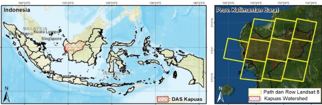
The location of the study was the Kapuas watershed in West Kalimantan Province (Figure 1). Kapuas watershed is the largest watershed on the island of Kalimantan, with an area of approximately 99129.78 Km2 or 70 % of the areas of West Kalimantan Province. This research requires about 10
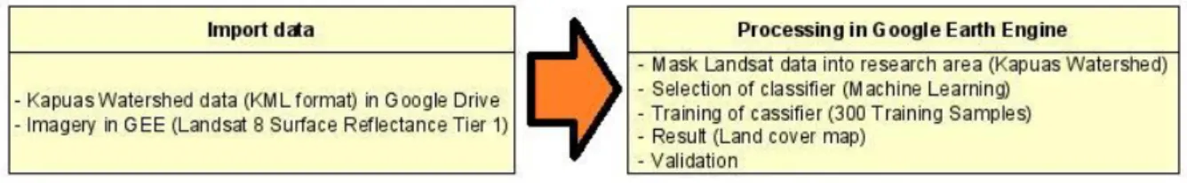
Landsat 8 satellite imagery scenes. The Landsat 8 satellite imagery data used in the study is recording 2019 and from USGS Landsat 8 Surface Reflectance Tier 1. Landsat 8 USGS Surface Reflectance Tier 1 imagery is ready to use because orthorectified and reflective calibration has processed.
GEE has accessed through this website www.earthengine.google.com. Before you can use GEE services, we asked to register first, and the results of the registration will be reviewed first by Google. After the registration and review process is complete, we can use GEE services such as satellite image processing through the code editor through this website www.code.earthengine.google.com. Through this code editor, we can analyze, create spatial data prototypes, and visualize them using JavaScript. This study uses a script compiled by Levick et al. (2019) and Farda (2020). In general, the step in this research is shown in Figure 2.
Fig. 1. Research Sites 2.2 Machine Learning Algorithm
Machine learning is one of the applications of artificial intelligence. The primary ability of machine learning is to handle high-dimensional data such as remote sensing data and map it into several classes with complex characteristics (Maxwell et al., 2018).
GEE provides a lot of machine learning, namely Fast Naive Bayes, CART (Classification and Regression Tree), Random Forests, GMO Max Entropy, Perceptron (Multi-Class Perceptron), Winnow, Pegasos (Primal Estimated Sub-Graded Sectors for SVM), IKPamir (Intersection Kernel) Passive Aggressive Method for Information Retrieval, SVM), Voting SVM and Margin SVM (Farda, 2017;
Shelestov et al., 2017). But this research does not use all available machine learning. The machine learning used in this study is logic-based machine learning (CART, Random Forest, GMO Max Entropy) and Support Vector Machine (Voting SVM, Margin SVM). The machine learning from GEE, which is most commonly used sequentially, is random forest and CART (based on logic) and then SVM (Tamiminia et al., 2020). Besides, the study of Farda (2017) shows that machine learning based on logic and SVM has better accuracy compared to perceptron-based (Winnow, Perceptron) and statistic-based (Fast Naïve Bayes).
Tabel 1. The combination of bands tested in this study.
Combination 1 Combination 2 Combination 3 Combination 4
Band 1 (Coastal) Band 2 (Blue) Band 3 (Green) Band 4 (Red) Band 5 (NIR) Band 6 (SWIR-1) Band 7 (SWIR-2) Band 10 (TIR-1) Band 11 (TIR-2) Band 2 (Blue) Band 3 (Green) Band 4 (Red) Band 5 (NIR) Band 6 (SWIR-1) Band 7 (SWIR-2) Band 1 (Coastal) Band 2 (Blue) Band 3 (Green) Band 4 (Red) Band 5 (NIR) Band 6 (SWIR-1) Band 7 (SWIR-2) Band 2 (Blue) Band 3 (Green) Band 4 (Red) Band 5 (NIR) Band 6 (SWIR-1) Band 7 (SWIR-2) Band 10 (TIR-1) Band 11 (TIR-2)
392 Fariz and Nurhidayati / JAGI Vol 4 No 2/2020 Fig. 2. Workflow of research method
In addition to comparing machine learning, this study also examined the combination of bands used (Table 1). Hu & Hu (2019) used all bands (except panchromatic and cirrus bands) on Landsat 8 satellite imagery to map land coverage while Shelevtov et al. (2017) and Kamal et al. (2020) only used bands 2 to band 7. Therefore we assume it is necessary to also compare the best band combinations for mapping ground cover using machine learning.
2.3 Research Sample
Land coverage mapped in this study only consists of 4 classes, namely water bodies, vegetation cover, open land, and land built or hardened. This land coverage class is the first order from a land coverage class based on spectral dimensions based on Danoedoro (2006).
Several classification processes using machine learning, several classification samples (training samples) are needed. The classification samples used in this study were 300 sample points. According to the classification sample, a test sample also taken to test the accuracy of the classification results. The
number of test sample points in this study was 200 points. This number refers to Congalton (2001) and Story & Congalton (1986), which states that the minimum sample size is 50 samples per class of land coverage.
3. Results and Discussions
3.1 Mapping land coverage using GEE machine learning
The stage of land coverage mapping with GEE begins by calling Landsat 8 satellite imagery from the USGS Landsat 8 Surface Reflectance Tier 1 collection. The challenge of land coverage mapping in the Kapuas watershed is that there is so much cloud cover that the satellite imagery used must go through the process of cloud masking and cloud shadow masking. Next is to do an image reducer using a median to reduce the collection of images by calculating the median of all image pixel values in a specific period. This function is useful for obtaining cloud-free images in 2019, high reflectance values, and shadows (Figure 3).
Fig. 3. The appearance of Landsat 8 satellite imagery before (A) and after (B) cloud masking and median processes Land coverage maps were tested for accuracy
using 200 test samples. The accuracy test results show that machine learning that was tested in this study has an accuracy above 0.85 in each combination. This might be due to the number of mapped land coverage classes that are still very common. The best accuracy in this study was obtained from GMO Max Entropy machine learning in combination 1. If viewed only based on the type of machine learning, then the GMO Max Entropy
machine learning has the best accuracy in this study followed by CART then SVM Voting. Suppose seen only based on the combination of the bands used, the combination of 3 consisting of band 1 (coastal) to band 7 (SWIR-2), which has the best accuracy in this study. This band combination is in line with the combination of bands 1 to band 7 in Landsat imagery, which has the best accuracy in discriminating land coverage class (Yu et al. 2019).
Table 2. The results of accuracy testing of land coverage mapping using machine learning.
All machine learning that was tested in this study did have an accuracy above 0.80, but if it is paid close attention, there are still misclassifications such as bodies of water classified as open land and open land classified as built-up (Figure 4). This is because the two objects have the same spectral appearance. Land coverage mapping with by variety detailed class in the Kapuas watershed will be challenging because of some objects such as rice fields, moor, oil palm plantations, and industrial forestry (HTI) have the same spectral appearance. Agricultural land has a
spectral appearance that varies depending on time, such as the planting period in the fields. So to get the results of mapping with good accuracy is by visual interpretation, although it will take a long time. Another solution is to use several other approaches, such as Geographic-Object-Based Image Analysis (GEOBIA). GEOBIA classifies land coverage classes not only by spectral but also object associations, although GEOBIA does not promise to provide high accuracy mapping of complex land coverages such as wetlands (Farda et al., 2016).
Fig. 4. The appearance of Landsat 8 satellite imagery before (A) and after (B) cloud masking and median processes
The accuracy test method used in this study can also be said to be too general. This makes the results of the mapping seem to have high accuracy. Mapping accuracy test results using kappa calculations have many shortcomings because they are only based on the randomness of the allocation and the randomness of the distribution (Pontius Jr & Millones, 2011). This makes Estes (1992) state that the accuracy of the test results has not answered which parts are accurate and which parts are less accurate (Danoedoro, 2012). 3.2 Conditions of land coverage in the Kapuas watershed
Mapping land coverage using GEE is far more efficient than the conventional method that starts with downloading satellite images and then processing them in GIS software. In addition, the cloud-based GEE platform facilitates extensive data processing,
such as the Kapuas watershed, which requires approximately 10 Landsat 8 image scenes.
Table 3. Land coverage class area.
Class Area (Km2)
Built-up area 206.46
Vegetation 93724.33
Water bodies 1592.88
Non-vegetated Area (barren land) 2917.05
No Data 689.05
Total 99129.78
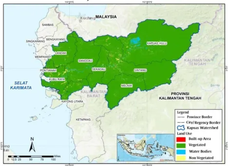
The map of land coverage in the Kapuas watershed in this study uses GMO Max Entropy machine learning and combination 1. The most extensive land coverage class is vegetation cover with an area of 9372.33 Km2 (Table 3). In addition there
Machine learning Overall Acuracy Average
Combination 1 Combination 2 Combination 3 Combination 4
Random Forest 0.90 0.89 0.93 0.88 0.90
GMO Max entropy 0.98 0.97 0.97 0.98 0.97
CART 0.90 0.96 0.95 0.90 0.93
SVM Voting 0.93 0.90 0.93 0.90 0.91
SVM Margin 0.89 0.87 0.89 0.87 0.87
394 Fariz and Nurhidayati / JAGI Vol 4 No 2/2020 are also no data classes with an area of 689.05 Km2.
No data is the appearance of cloud masking images. The large amount of cloud cover at the study site
causes the appearance of clouds even though the selected image has been reduced using a median.
Fig. 5. Map of land coverage in the Kapuas watershed On the map of land coverage in the Kapuas
watershed (Figure 4), it is seen that in the upstream area of the Kapuas watershed (which is administratively located in the Kapuas Hulu Regency) is still dominated by vegetation land coverage classes. Although dominated by vegetation land coverage, this land coverage map cannot yet indicate the criticality of the watershed because the land coverage class is still common. Therefore, it is necessary to map land coverage in the Kapuas watershed with more specific land coverage classes, which divide vegetation cover into agricultural and non-agricultural land. It indicates the criticality of the Kapuas watershed because almost all critical watersheds have the same problem, namely changes in land coverage in the upstream and areas along the river banks (Setyowati et al., 2019).
This study still has many shortcomings, such as a period that is only one time. This research developed using more diverse input data such as image transformation and more detailed land coverage classes such as Hu & Hu (2019) and Farda (2017). In addition, it is also necessary to test the hyperparameter between machine learning, such as the study of Shih et al. (2019).
4. Conclusions
GEE, with the machine learning, that it provides, can process images quickly even though the scope of the area is vast. This will certainly facilitate the process of inventory information on land coverage in the Kapuas watershed, which has a vast area and a lot of cloud cover. The results of this study indicate that the best machine learning in mapping land coverage in the Kapuas watershed is GMO Max Entropy, then CART. The combination of bands that have the highest accuracy is a combination of bands 1 to band 7.
This research still has many limitations, especially mapped land coverage classes. So that research needs to be developed with more detailed land coverage classes, more diverse and multi-time input data.
References
Congalton, R. G. (2001). Accuracy assessment and validation of remotely sensed and other spatial information. International Journal of Wildland Fire, 10(4), 321-328.
Danoedoro, P. (2006). Versatile Land-use Information for Local Planning in Indonesia. Disertasi. Centre for Remote Sensing and Spatial Information Science (CRSSIS). School of Geography, Planning and Architecture. The University of Queensland. Danoedoro, P. (2012). Pengantar penginderaan jauh
digital. Yogyakarta: Penerbit Andi
Effendi, E. (2008). Kajian Model Pengelolaan Daerah Aliran Sungai (DAS) Terpadu. Direktorat Kehutanan dan Konservasi Sumberdaya Air, Badan Perencanaan Pembangunan Nasional. Jakarta.
Estes J. (1992). Remote sensing and GIS Integration: Research Needs, Status and Trends. ITC Journal (3)
Farda, N. M. (2017). Multi-temporal land use mapping of coastal wetlands area using machine learning in Google earth engine. IOP Conference Series: Earth and Environmental Science (Vol. 98, No. 1, p. 012042). IOP Publishing.
Farda, N. M. (2020). Image classification – Machine
learning. Accessed from
code.earthengine.google.com/?accept_repo=u sers/farda/EE03 at 9 July 2020
Farda, N. M., Danoedoro, P., Harjoko, A. (2016). Image mining in remote sensing for coastal wetlands mapping: from pixel based to object based approach. IOP Conference Series: Earth and Environmental Science (Vol. 47, No. 1, p. 012002). IOP Publishing.
Gastellu-Etchegorry, J. P. (1988). Predictive models for remotely-sensed data acquisition in Indonesia. International Journal of Remote Sensing, 9(7), 1277-1294.
Hu, Y., & Hu, Y. (2019). Land cover changes and their driving mechanisms in Central Asia from 2001 to 2017 supported by Google Earth Engine. Remote Sensing, 11(5), 554.
Kamal, M., Farda, N. M., Jamaluddin, I., Parela, A., Wikantika, K., Prasetyo, L. B., & Irawan, B. (2020). A preliminary study on machine learning and google earth engine for mangrove mapping. IOP Conference Series: Earth and Environmental Science (Vol. 500, No. 1, p. 012038). IOP Publishing.
Levick, S. R., Bae, S., Guderle, M., Singh, J., Luck, L. 2019. Introduction to remote sensing of the
environment. Accessed from
geospatialecology.com at 14 July 2020 Maxwell, A. E., Warner, T. A., & Fang, F. (2018).
Implementation of machine-learning classification in remote sensing: An applied review. International Journal of Remote Sensing, 39(9), 2784-2817.
Pemerintah Republik Indonesia. 2015. Peraturan Presiden Republik Indonesia Nomor 2 Tahun 2015 tentang Rencana Pembangunan Jangka
Menengah Nasional Tahun 2015 – 2019.
Sekretariat Negara: Jakarta
Pontius Jr, R. G., Millones, M. (2011). Death to Kappa: birth of quantity disagreement and allocation disagreement for accuracy assessment. International Journal of Remote Sensing, 32(15), 4407-4429.
Poongothai, S., Sridhar, N., & Shourie, R. A. (2014). Change detection of land use/land cover of a watershed using remote sensing and GIS. Inter. J. Engg. Adv., Tech, 3(6), 226-230. Setyowati, D. L., Amin, M., Suharini, E., & Pigawati,
B. (2012). Model Agrokonservasi Untuk Perencanaan Pengelolaan Das Garang Hulu. TATALOKA, 14(2), 131-141.
Setyowati, D. L., Arsal, T., Hardati, P., & Prabowo, K. Z. (2019). Morphoconservation analysis on Kali Garang as a river conservation effort. In IOP Conference Series: Earth and Environmental Science (Vol. 243, No. 1, p. 012007). IOP Publishing.
Shelestov, A., Lavreniuk, M., Kussul, N., Novikov, A., & Skakun, S. (2017). Exploring Google Earth Engine platform for big data processing: Classification of multi-temporal satellite imagery for crop mapping. frontiers in Earth Science, 5, 17.
Shih, H. C., Stow, D. A., & Tsai, Y. H. (2019). Guidance on and comparison of machine learning classifiers for Landsat-based land cover and land use mapping. International Journal of Remote Sensing, 40(4), 1248-1274. Story, M., & Congalton, R. G. (1986). Accuracy
assessment: a user’s
perspective. Photogrammetric Engineering and remote sensing, 52(3), 397-399.
Talukdar, S., Singha, P., Mahato, S., Pal, S., Liou, Y. A., & Rahman, A. (2020). Use Land-Cover Classification by Machine Learning Classifiers for Satellite Observations—A Review. Remote Sensing, 12(7), 1135. Tamiminia, H., Salehi, B., Mahdianpari, M.,
Quackenbush, L., Adeli, S., & Brisco, B. (2020). Google Earth Engine for geo-big data applications: A meta-analysis and systematic review. ISPRS Journal of Photogrammetry and Remote Sensing, 164, 152-170.
Yu, Z., Di, L., Yang, R., Tang, J., Lin, L., Zhang, C., ... & Sun, Z. (2019). Selection of Landsat 8 OLI Band Combinations for Land Use and Land Cover Classification. In 2019 8th International Conference on Agro-Geoinformatics (Agro-Geoinformatics) (pp. 1-5). IEEE.