ISSN 1440-771X
Australia
Department of Econometrics and Business Statistics
http://www.buseco.monash.edu.au/depts/ebs/pubs/wpapers/
May 2010
Do Jumps Matter? Forecasting Multivariate
Realized Volatility allowing for Common Jumps∗
Do Jumps Matter? Forecasting Multivariate
Realized Volatility allowing for Common Jumps
∗
Yin Liao
School of Economics
Australian National University
Australia
Heather M. Anderson and Farshid Vahid
Department of Econometrics and Business Statistics
Monash University
Australia
†May 2010
Abstract
Realized volatility of stock returns is often decomposed into two dis-tinct components that are attributed to continuous price variation and jumps. This paper proposes a tobit multivariate factor model for the jumps coupled with a standard multivariate factor model for the continu-ous sample path to jointly forecast volatility in three Chinese Mainland stocks. Out of sample forecast analysis shows that separate multivariate factor models for the two volatility processes outperform a single mul-tivariate factor model of realized volatility, and that a single mulmul-tivariate factor model of realized volatility outperforms univariate models.
Keywords: Realized Volatility, Bipower Variation, Jumps, Common Factors, Forecasting
JEL classification: C13, C32, C52, C53, G17, G32
∗We thank Jeff McGill, Bruce Mizrach, Adrian Pagan, Tom Smith and participants of
the ANU School of Economics Brown Bag Seminar Series, the Financial Integrity Research Network Time Series workshop and the Chicago-London workshop on Financial Markets for useful comments and suggestions. We also acknowledgefinancial assistance from the Aus-tralian Research Council, for Discovery Grants # DP0449995 and #DP0665710.
†E-mail: [email protected], [email protected], [email protected]
1
Introduction
Recent literature on the second moment of an asset’s price has focussed on realized volatility as a measure of volatility in returns. Increased interest in this measure of volatility is due to new advances in theory that show that realized volatility can provide a consistent estimate of integrated volatility in a standard continuous time diffusion model of (the logarithm of) an asset’s price. Further, the fact that realized volatility is particularly easy to calculate has also contributed to its rise in popularity. Given the need for frequent and timely volatility forecasts when pricing and managing the risks associated with holding portfolios, there is now a large and growing literature that attempts to model and then forecast realized volatility1. With the growth of this literature has come recognition of the role that jumps can play in the price processes for assets, and their consequent role in the generation of volatility.
The standard continuous-time jump diffusion models assume that the dy-namic characteristics of jumps are quite different from those of the continuous portion of the price process, but in practice the jumps are usually ignored or simply removed when building forecasting models of volatility. Recent excep-tions can be found in work undertaken by Andersen, Bollerslev and Huang (2007) and Lanne (2007), who show that volatility forecasting can benefit from separately modeling and forecasting the two variation sources. These empirical findings are not surprising, given that the assumptions imposed on the jumps and the continuous portions of price imply that one should expect each compon-ent to play a differcompon-ent role in forecasting. Most empirical studies that separate realized volatility into continuous and jump componentsfind that the volatility due to the continuous component of the price process is very persistent, whereas the jump component is essentially serially uncorrelated. Nevertheless, Andersen at al (2007)find that the time between jumps is predictable, and Lanne (2007) finds persistence in the size of the jump volatility components in his data set.
The above cited work develops forecasting models that are useful in univari-ate settings, and extensions that can forecast volatility in multivariunivari-ate settings are potentially useful, especially sincefinancial phenomena are inherently mul-tivariate. Factor models provide an attractive starting point given their strong theoretical basis in the finance literature, and they provide parsimony when modeling comovement in large data sets. Recent work by Anderson and Vahid (2007) and Marcucci (2008) shows that factor models can be useful for modeling and forecasting the continuous components of volatility in large sets of stock re-turns. Further, there is now a developing literature due to Bollerslev, Law and Tauchin (2008), Jacod and Todorov (2009) and others, who test for and find evidence of co-jumps. This suggests that factor models of jumps have empirical relevance, and lays open the possibility that they might have forecasting po-tential. One objective of this paper is to explicitly model the volatility arising from jumps in a multivariate framework, and then to examine whether a factor model of the jump process can contribute to forecasts of realized volatility.
The theory relating to the decomposition of realized volatility into continu-ous and jump components has now been well developed in a series of papers by Barndorff-Nielsen and Shephard (2002a, 2002b, 2004, 2006), although the measurement of jumps is problematic in practice. The most straightforward way to measure jumps is to subtract bi-power variation (defined below) from realized volatility, but this procedure often leads to theoretically incorrect negat-ive measures of jumps. These negatnegat-ive measures are set back to zero to partially correct for this measurement error, with the result that the "corrected" jump measure contains zeros. The presence of these zeros is, however, consistent with the intuition that jumps need not occur during all time periods. Indeed, some studies take the view that jumps should only occur occasionally, so they set most of their jump series equal to zero and then let jumps be positive, only when jump tests have identified statistically significant departures from zero.
The challenge associated with constructing a common factor model for jumps lies in dealing with series that theoretically consist of either zero or positive ob-servations, because standard techniques for estimating unobserved factors such as principle components do not make allowance for this. We proceed by treating the observed non-negative jump series as censored variables and then develop a factor model based on a multivariate Tobit specification. An important feature of this model is that it can only predict non-negative jumps, consistent with the intuition that jumps in volatility cannot be negative. We discuss the es-timation of this tobit type factor model and show that this involves adapting standard Kalmanfiltering procedures that are typically used to estimate factors, to separately account for zero and non-zero observations. Our procedure is com-putationally feasible for “small-N”2 data sets, and we demonstrate how it works by building and estimating a factor model for a trivariate system of jumps.
Our empirical application is based on high frequency returns relating to three medical stocks sold on the Chinese mainland stock exchange. We use this data because our previous research (Liao, 2008) has found that the jumps in this emerging market are more frequent and predictable than those in developed financial markets, so we have good reason to suspect that jumps might play a strong role in forecasting realized volatility in this setting. We build a series of forecasting models for realized volatility, some of which are univariate, some of which are multivariate, and some of which are comprised of separate factor models for bi-power variation and jumps. We then undertake some forecast analysis to assess how the separate forecasting of jumps contributes to forecasts of total realized volatility, and how our tobit type model fares relative to other factor models. We find that separate treatment of jumps is useful, and that although our factor model does not outperform an equally weighted factor model of the multivariate jump process, it nevertheless makes a positive contribution towards the forecasting of jumps and realized volatility.
The rest of this paper is structured as follows. Section 2 discusses how to extract the jump series from realized volatility, and describes our common factor model for jumps. Section 3 provides a description and a preliminary analysis
of our data. Section 4 develops univariate and multivariate factor models for total realized volatility, the underlying continuous sample path and jumps re-spectively, and then compares their out-of-sample performance with respect to forecasting realized volatility. Section 5 concludes.
2. Jumps
In this section, we discuss the way in which we extract jumps from realized volatility, and the way in which we model and estimate our multivariate tobit factor model of jumps.
2.1 Decomposing Realized Volatility
We assume that the logarithm of the asset price within the active part of the trading day evolves in continuous time as a standard jump-diffusion process given by
dp(t) =u(t)dt+σ(t)dw(t) +κ(t)dq(t), (1) where u(t) denotes the drift term that has continuous and locally bounded variation,σ(t)is a strictly positive spot volatility process andw(t)is a standard Brownian motion. Theκ(t)dq(t)term refers to a pure jump component, where
k(t) is the size of jump and dq(t) = 1 if there is a jump at time t (and 0 otherwise). The corresponding discrete-time within-day geometric returns are
rt+j4=p(t+j/M)−p(t+ (j−1)/M), j= 1,2, ....M, (2)
where M refers to the number of intraday equally spaced return observations over the trading dayt,and∆= 1/M denotes the sampling interval. As such, the daily return for the active part of the trading day equalsrt=PMj=1rt+j4.
As noted in Andersen and Bollerslev (1998), Andersen, Bollerslev, Diebold and Labys (2003), and Barndorff-Nielsen and Shephard (2002a, b), the volatility over the active part of the trading daytcan be measured by realized variance, which converges uniformly in probability to quadratic variation as the sampling frequency goes to infinity. Realized volatility (RV) is defined as the sum of the intraday squared returns, i.e.
RVt+1(∆)≡
M
X
j=1
rt2+j∆. (3)
We need a consistent estimator of integrated volatility which is robust even in the presence of jumps in order to extract the jump component from the realized volatility. Barndorff-Nielsen and Shephard (2004, 2006) proposed realized bi-power variation (RBV), defined as the sum of the product of adjacent absolute intraday returns standardized byμ1≡p2/Π≈0.79788as a suitable measure, and in the work below we use a variation of this measure given by
RBVt+1(∆)≡μ−12( M M−2) M X j=3 |rt+j∆||rt+(j−2)∆|→ Z t+1 t σ2(s)ds. (4)
Relative to the original measure considered in Barndorff-Nielsen and Sheph-ard (2004), the bipower variation measure defined above involves an additional lagging strategy suggested by Huang and Tauchen (2005), because this helps to correct for market microstructure bias. The difference between realized variance and realized bipower variation consistently estimates the part of the quadratic variation due to jumps so that
RVt+1(∆)−RBVt+1(∆)→
X
t<s<t+1
κ2(s). (5)
As this difference can take negative values, we follow the suggestion made by Barndorff-Neilsen and Shephard (2004) and truncate the empirical measurement at zero. Thus the jump series is estimated by
Jt+1(∆) =max[RVt+1(∆)−RBVt+1(∆),0]. (6)
The continuous sample path component Ct+1(∆) is consistently estimated by
realizedRBVt+1(4),but to maintain the property that the continuous and jump
components sum to realized volatility, we adjust the continuous component to account for the removal of the negative jumps. Given that our primary purpose is simply to forecast realized volatility, we do not further adjust our series to extract statistically significant jumps.
2.2 Tobit Common Factor Model of Jumps
Factor models were originally designed for large dimension data sets, and they aim to describe the observed comovement in a large set of series in terms of a small number of unobserved common factors. We follow this idea, butfirst need to recognize that jumps are non-negative. This leads us to work with a baseline set-up that is similar to a tobit model that is specified by
Jit={ J∗ it Jit∗ >0 0 J∗ it≤0 (7) Jt∗=ΛFt+ut. (8) In this specification, J∗
t is an N×1vector of a continuous underlying random variable that is only observed if it is larger than zero, Jt is the corresponding
N×1vector of our observations on jumps, Ft= (F1t...Frt)is anr×1vector of common factors,Λ is anN×rmatrix of factor loadings andutis anN×1 vector of idiosyncratic factors that are independent ofFt. A strict factor model would assume thatutis a vector of serially uncorrelated errors withE(ut) = 0 and E(utu
0
t) = Σ =diag(σ21, ...., σ2N), but these fairly restrictive assumptions can be relaxed when the dimension of the data set is large (see Chamberlain and Rothschild (1983) for a discussion on approximate factor models). In this latter case it is possible to allow for (weak) serial and cross correlation of the idio-syncratic errors, and weak correlation among the factors and the idioidio-syncratic components. In our case we are jointly modeling three series, and we assume
a single common factor (since a scree plot indicates that only one eigenvalue of the sample correlation matrix is larger than unity, and a one factor model seems likely in this setting). We assume that the factor and the idiosyncratic com-ponents are contemporaneously uncorrelated, although we allow each to follow dynamic processes, and hence allow for serial correlation inuit.
Our model then consists of equation (7), and equations (9) and (10) given below,
Jit∗ =αift+uit (9)
ft=b0+b1ft−1+....+bpft−p+γ1 t−q+γ2 t−q+1+....+ t (10) and one of the key features of this model is that it will always deliver non-negative forecasts, in line with the intuition that our jump forecasts should take non-negative values.
2.2.1 Estimation
This kind of model admits a state-space representation, with a measurement equation given by Jt∗= ¡ α , 0 ¢St+ut (11) with (α,0) = ⎛ ⎜ ⎜ ⎜ ⎜ ⎝ α1 | 0 · · · 0 α2 | ... ... .. . | ... . .. ... αn | 0 · · · 0 ⎞ ⎟ ⎟ ⎟ ⎟ ⎠ and St = ⎛ ⎜ ⎜ ⎜ ⎜ ⎜ ⎜ ⎜ ⎜ ⎝ ft .. . ft−p t−q .. . t ⎞ ⎟ ⎟ ⎟ ⎟ ⎟ ⎟ ⎟ ⎟ ⎠ , and a transition equation given by St=β1+β2St−1+vt (12) withβ1= ⎛ ⎜ ⎜ ⎜ ⎜ ⎜ ⎜ ⎜ ⎜ ⎜ ⎜ ⎝ b0 0 .. . −− 0 .. . 0 ⎞ ⎟ ⎟ ⎟ ⎟ ⎟ ⎟ ⎟ ⎟ ⎟ ⎟ ⎠ andβ2= ⎛ ⎜ ⎜ ⎜ ⎜ ⎜ ⎜ ⎜ ⎜ ⎜ ⎜ ⎜ ⎜ ⎝ b1 · · · bp−1 bp | γ1 · · · γq 0 | Ip−1 ... | 0 0 | − − − − | − − − | 0 0 | ... Iq−1 | 0 · · · 0 ⎞ ⎟ ⎟ ⎟ ⎟ ⎟ ⎟ ⎟ ⎟ ⎟ ⎟ ⎟ ⎟ ⎠ .
The error terms satisfyE(u0) = 0, E(u0u) = R, E(υ) = 0 and E(v0v) = Q. The assumption that J∗ is normally distributed would allow us to estimate the unknown factor and coefficients of the common factor model via Gaussian maximum likelihood using the Kalman Filter, if the vector J∗ was observed. However, the elements ofJ∗are only observed when they are positive, so we have
to modify the standard estimation procedure to accommodate the information behind the truncation mechanism.
2.2.2 The log-likelihood function based on the time series of jumps The log-likelihood function for a sample{Jt, t= 1, . . . , T}is
lnL(θ|JT,JT−1, . . . ,J1) = lnD(JT,JT−1, . . . ,J1;θ) = T X t=1 lnD(Jt| It−1;θ)
where D(.) is the joint probability density function, D(.| It−1)is the
condi-tional density given the observed information at timet−1andθ is the vector of model parameters. For eacht,Jt is a vector of jumps inN volatilities, and some of the elements ofJtwill be exactly zero, even though most will be strictly positive. We letX0tandX+tdenote the sets of indices for assets with no volat-ility jumps and positive volatvolat-ility jumps at timet,i.e. X0t={i:Jit= 0}and
X+t = {i:Jit>0}, and let N0t and N+t denote the cardinality of X0t and
X+t.Note that either of these sets (but not both) can be empty and their inter-section is empty, butX0t∪X+t={1,2, . . . , N},implying thatN0t+N+t=N. We takeN0trows of theN×N identity matrix corresponding to the indices in
X0tand stack them into a matrixX0tand then we stack the otherN+trows of the identity matrix into a matrixX+t. This ensures thatX0tJtselects theN0t subvector ofJt whose elements are all zero andX+tJtselects allN+t non-zero elements ofJt. By definition, we can then write each term in the likelihood as
D(Jt| It−1) =D(X0tJt|X+tJt, It−1)×D(X+tJt| It−1).
We now assume that the underlyingN×1vectorJ∗
t is normally distributed3, with a conditional mean J∗
t|t−1 and conditional varianceGt|t−1. Then for i =
1,2, . . . , N, we have
D(X0tJt|X+tJt,It−1) = P r(X0tJ∗t ≤0|X+tJ∗t,It−1), and
D(X+tJt| It−1) = D(X+tJ∗t | It−1).
Conditional on the information at timet−1,the means ofX0tJ∗t andX+tJ∗t are
X0tJ∗t|t−1andX+tJ∗t|t−1,their variances areX0tGt|t−1X00t andX+tGt|t−1X0+t, and their covariance isX0tGt|t−1X0+t.Joint normality implies that the density
D(X0tJ∗t |X+tJ∗t, It−1)is also normal with
E(X0tJ∗t |X+tJ∗t, It−1) =X0tJ∗t|t−1 +X0tGt|t−1X0+t ¡ X+tGt|t−1X0+t ¢−1³ X+tJ∗t−X+tJ∗t|t−1 ´ V(X0tJ∗t |X+tJ∗t, It−1) =X0tGt|t−1X00t −X0tGt|t−1X0+t ¡ X+tGt|t−1X0+t ¢−1 X0 +tGt|t−1X0t
3This is unlikely to be true in our application, but it simplifies the analysis and paves the
Cov(X0tJ∗t, X+tJ∗t |X+tJ∗t, It−1) =X0tGt|t−1X01t −X0tGt|t−1X0+t ¡ X+tGt|t−1X0+t ¢−1 X0 +tGt|t−1X0t.
We use these expressions to calculate Pr (X0tJ∗t ≤0|X+tJ∗t, It−1) from this
N0tdimensional normally distributed random variable, which is relatively easy since there are fast algorithms for calculating the CDF for univariate, bivari-ate and trivaribivari-ate normal distributions. The second piece of the likelihood, i.e.
D(X+tJ∗t | It−1)is the PDF of an N+t dimensional normally distributed ran-dom variable with mean X+tJ∗t|t−1 and varianceX+tGt|t−1X0+t, evaluated at
X+tJt. The mean and variance of the distribution ofJ∗t conditional on It−1,
and conditional on the structure of the model are computed recursively using a slight modification of the Kalmanfilter explained below.
2.2.3 Kalman Filter Modification
Once the model has been put into a state space form, the Kalman filter is a good tool to recursively compute the optimal estimate of the latent state vector in each period, and the conditional mean and covariance matrix of the distribution of the observed vector based on the available information set. In the usual case in which the observed vector and the state vector have a linear relationship, the assumption that the disturbances and initial state vector are normally distributed implies that the mean of the conditional distribution of the state vector based on the observed vector is the maximum likelihood estimator of the state vector based on all the available information. To start the Kalman filter, we usually set the initial state vector equal to the mean and covariance matrix of the unconditional distribution of the state vector, i.e. S0|0 = (I−
β2)−1β
1andvec(P0|0) = (I−β2⊗β2)−1vec(Q)in the state space model outlined
in Section 2.2.1., where ⊗ is the Kronecker product and the vec(.) operator indicates that the columns of the matrix are being stacked one upon the other. If J∗
t was fully observed, the latent state vector St and the observed vector
J∗
t could be predicted in each period, and the prediction could be updated iteratively once the actual observed vector is available in next period. The standard recursive procedure is explained in Appendix A.
The standard Kalmanfilter can not be used in the current situation because the observed Jt are sometimes censored values of Jt∗, and this prevents the direct calculation of some of the one step prediction errors. Since the prediction errors (et|t−1) in each period are used for updating, the calculation of these
errors needs to be modified to allow updating to occur. We do this by noting that the zeros provide the information that the corresponding elements of J∗
t are truncated values, so we use the truncated expected value of J∗
t based on the information up to the current period as an estimate ofJ∗
t that is then used to calculate the expected one-step ahead prediction error. The mathematical analysis of this procedure is provided in Appendix C. Note that simply using zeros as the actual values or treating them as missing data would lead to biased estimation, whereas the use of the information hidden behind the zeros corrects for this.
cases, i.e. jumps occur in all the assets, jumps do not occur in any of the assets, or jumps occur in some but not all assets. We separately consider the updating step of the Kalmanfilter for each of these cases below.
Case 1 - There are positive jumps in all assets at time t: In this case, each element ofJ∗
t can be observed. Hence, the vector of prediction errorset|t−1can
be calculated as the difference between the observed value ofJt and the value ofJ∗
t|t−1 predicted at time t-1. The rest of the updating procedure is the same
as the standard one and is
St|t=E(St|It−1) +Cov(St,J∗t)V ar(J∗t)et|t−1 =St|t−1+Pt|t−1α 0 G−t|t1−1(J∗ t−J∗t|t−1) Pt|t=V ar(St|It−1)−Cov(St,J∗t)V ar(J∗t)Cov(St,J∗t) 0 =Pt|t−1−Pt|t−1α 0 Gt|t−1αP 0 t|t−1.
Case 2 - No assets have jumps at timet: In this case, each of theN elements in the vector of jumpsJtis truncated at zeros and J∗t can not be observed. The
only new information from the zeros is that all elements ofJ∗
t of all the assets
at time t are negative. Hence, we use the truncated conditional expected values to update the estimate of the state vector and its covariance matrix using
St|t=E(St|J∗t ≤0,It−1) =St|t−1+Pt|t−1α 0 G−t|t1−1(E(J∗t|Jt∗≤0,It−1)−J∗t|t−1) Pt|t=V ar(St|J∗t ≤0,It−1) =Pt|t−1−Pt|t−1α 0 G−t|t1−1(Gt|t−1−V ar(J∗t|J∗t ≤0,It−1)) 0 G−t|t1−1αP0 t|t−1 where E(J∗
t|J∗t ≤0,It−1) is the truncated conditional mean of the vectorJ∗t, and V ar(J∗
t|J∗t ≤ 0,It−1) is the truncated conditional variance of the vector
J∗
t.4
Case 3 - Some of the assets have no jumps, but the rest of them have positive jumps: As in section 2.2.2, we extract two submatricesX0t andX+t from the identity matrix to split the vector Jt into two subvectors X0tJt and X+tJt, which respectively select all zero elements and non-zero elements of Jt. For the non-zero subvector ofJt, the vector of prediction errors at time t can be calculated using the standard procedure, whereas the vector of prediction errors for assets with no jumps is calculated by taking the difference between the truncated conditional meanE(X0tJ∗t | X0tJ∗t ≤0, X+tJ∗t,It−1) based on the
information set at time t and the predicted value X0tJ∗t|t−1. The conditional distribution needed to calculate this expectation is normally distributed as in section 2.2.2, but in addition to the conditioning done before, we now have to condition on our knowledge thatX0tJ∗t ≤0as well.
4E(J∗
t|J∗t ≤0,It−1) =Jt∗|t−1−SJRJH(SJ−1(0−J∗t|t−1))and V ar(J∗t|J∗t ≤0,It−1) =
Gt|t−1−SJRJ∇H(SJ−1(0−J∗t|t−1))0SJRJ, whereSJ is the diagonal matrix of the square
roots of the elements of the covariance matrix(Gt|t−1)ofJt∗,conditional on the information
available at timet−1andRJ is the corresponding correlation matrix ofGt|t−1. H(.)is the multivariate hazard rate,H(α) = ∇ΦΦ((αα)), whereΦ(α) is the multivariate joint cumulative density function of the vectorαand∇Φ(α)is the gradient vector ofΦ(α)evaluated at the vector ofα.∇[H(SJ−1(0−J∗
t|t−1)]
0
is the matrix offirst partial derivatives of the elements of
H(S−J1(0−J∗
To do this, we defineS to be the diagonal matrix that contains the square roots of the elements of conditional covariance matrixV (X0tJ∗t |X+tJ∗t,It−1)
in (11) andRto be the corresponding correlation matrix obtained from the same matrix. We treat the conditional covariance matrixCov(X0tJ∗t,X+tJ∗t |X+tJ∗t,It−1)
in (11) similarly, and define S1 to be the diagonal matrix that contains the
square roots of the elements of this matrix andR1to be the corresponding
cor-relation matrix. Then if we denote ∇ΦΦ(α(α)) byH(α),the appropriate conditional distribution has moments given by
E(X0tJ∗t |X0tJ∗t ≤0, X+tJ∗t,It−1) (13) =E(X0tJ∗t |X+tJ∗t,It−1)−SRH[S−1(0−E(X0tJ∗t |X+tJ∗t,It−1))] V =V ar(X0tJ∗t |X0tJt∗≤0, X+tJ∗t,It−1)) =V(X0tJ∗t |X+tJ∗t,It−1)−SR∇H[S−1(0−E(X0tJ∗t |X+tJ∗t,It−1))SR CV =Cov(X0tJt∗,X+tJ∗t |X0tJ∗t ≤0, X+tJ∗t,It−1)) =Cov(X0tJ∗t,X+tJ∗t |X+tJ∗t,It−1)−S1R1∇H[S−1(0−E(X0tJ∗t |X+tJ∗t,It−1))S1R1
The updating steps are now based on this conditional distributed, and are
St|t=E(St|X0tJ∗t≤0, X+tJ∗t,It−1) =St|t−1+Pt|t−1α 0 G−t|t1−1 Ã E(X0tJ∗t |X0tJ∗t ≤0, X+tJ∗t,It−1)−X0tJ∗t|t−1 X+tJ∗t −X+tJ∗t|t−1 ! andPt|t=V ar(St|X0tJt∗≤0, X+tJ∗t,It−1) =Pt|t−1−Pt|t−1α 0 G−t1 |t−1G M t|t−1Pt|t−1α 0 G−t1 |t−1 where GMt|t−1= ( X0tGt|t−1X 0 0t−V X0tGt|t−1X 0 +t−CV X0tGt|t−1X 0 +t−CV X0tGt|t−1X 0 +t ).
The computed conditional mean and variance of the distribution of J∗
t based on the updated state vector and its covariance matrix can be put into the log-likelihood function to estimate the parameters, as in Section 2.2.2.
2.2.3 Simulation Study
We undertake a small simulation study to show that the zeros will bias estima-tion based on the standard Kalmanfilter, and that the modified Kalmanfilter is able to correct the bias. To do this, we generate a simple common factor model based on yit={ y∗ it y∗it>0 0 y∗ it≤0 (14) yt∗=αft+et, ,et∼N(0, R) R= µ σ21 0 0 σ22 ¶ ,
ft=b1+b2ft−1+vt, ,vt∼N(0,1) , in which y∗
t is an N ×1(we set N = 2 for simplicity) vector of latent vari-ables measured at time t, and yt is only observed when it is larger than zero. The variableft is a q×1vector containing common factors (we set q= 1 for simplicity), αis an N×q factor loading matrix, and etis an N×1 vector of idiosyncratic errors that follows a multivariate normal distribution with mean zero and an N ×N covariance matrix R. The common factor is an AR(1) process andb2 is the autoregressive coefficient. We set the value of parameters
to be©α1= 0.05, α2= 0.25, σ21= 0.049, σ22= 0.081, b1= 0.1, b2= 0.8ª and
then after drawing a random variablev0 from a standard normal distribution,
the initial value of common factor is generated viaf0|0= 1−b1b2 +
q
1 1−b2
2v0. We generate samples ofytfor samples of T = 800, 5000 and 10000, and implement both the standard Kalman filter, and the modified Kalman filter to estimate the parameters and the underlying factorft.
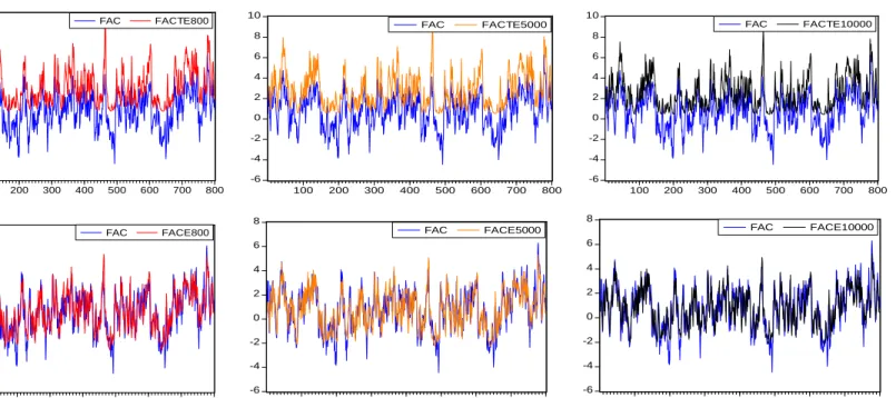
Table 1 shows that the estimates provided by the standard Kalmanfilter are seriously biased, regardless of the sample size. The estimates from the modified Kalmanfilter are much better and converge to the actual value as the sample size increases. Thus it appears that our modified Kalman filter is providing consistent estimates for the tobit state-space model. Figure 1 shows that the estimated common factors based on the standard Kalman filter do not take negative values, and hence they deviate from the generated underlying factor. On the other hand the estimated common factors based on the modified Kalman filter fit the generated factor better, and approach the actual factor with the increase of sample size. We apply our modified filter to estimate some state space common factor models of jumps in section 4.
3. Data
Our empirical analysis is based on intraday data on three individual stocks (SH600085, SH600351 and SZ000919)5in the Chinese stock exchange,6 whereas the existing literature related to realized volatility in Chinese mainland stock exchange is mostly based on market indices7 (see Zhang and Xu (2006), and Wang, Yao, Fang and Li (2006, 2008)). The raw transaction prices (together
5The full names of the companies are BEIJING TONGRENTANG CO., LTD, SHANXI
YABAO PHARMECEUTICAL (GROUP) CO., LTD, and JINGLIN PHARMECEUTICAL CO., LTD, which are three of the largest medicine manufacturingfirms in China. We choose these stocks for analysis because they have a long history of both operation (established in 1954) and listing (IPO dates back to 1997), and they are extensively traded. Firm details relating to trading on the SSE may be found on the websites http://www.sse.com.cn and http://www.szse.com.cn.
6There are two official stock exchanges in the Chinese mainland, i.e. the Shanghai Stock
Ex-change (SHSE) and the Shenzhen Stock ExEx-change (SZSE), which were established in December 1990 and July 1991 respectively. SH600085 and SH600351 are from SHSE, while SZ000919 is from SZSE.
7There are three main market indices in the Chinese stock market including the China
Securities Index (CSI 300) which is a market capitalization weighted index that measures the performance of the 300 of the most highly liquid A shares on both the Shanghai and the
with trading times and volumes) were obtained from the China Stock Market & Accounting Research (CSMAR) database provided by the ShenZhen GuoTaiAn Information and Technology Firm (GTA).
Trading in the Chinese Stock Exchange is conducted through the electronic consolidated open limit order book (COLOB), and it is carried out in two ses-sions with a lunch break. The morning session is from 09:30 to 11:30 and the afternoon session is from 13:00 to 15:00. Both exchanges are in the same time zone. Before the morning session, there is a 10-minute open call auction session from 09:15 to 09:25 to determine the opening price. The afternoon session starts from continuous trading without a call auction. The closing price of the active trading day is generated by taking a weighted average of the trading prices of the final minute. The market is closed on Saturdays and Sundays and other public holidays.
There are three main differences between Chinese mainland stock markets and Western developed stock markets when comparing them with respect to in-stitutional setting and trading rules, First, there is afive minute break between the periodic auction for the opening price and the normal morning session of continuous trading. In addition, there is a lunch break in the middle of the day between the morning and afternoon sessions, as in other Asian stock markets. Second, the market is an order-driven market that is entirely based on electronic trading, and it functions without market makers. Floor trading among member brokers and short selling are strictly prohibited. A further difference lies in a relatively immature infrastructure that embodies inadequate disclosure, and the coexistence of an inexperienced regulator with a limited number of informed in-vestors and an enormous number of uninformed inin-vestors. Given these market characteristics, the Chinese mainland stock exchange is expected to provide an interesting picture of an emerging stock market, that when compared to de-veloped markets might provide useful insights into a variety of issues associated with the trading of stocks.
We focus on the active trading period and leave issues associated with overnight volatility for further research. Paralleling many previous studies, we use five-minutes as the sampling frequency in an attempt to strike a reason-able balance between accurate measures and microstructure noise.8 Due to the
Shenzhen Stock Exchanges, the Shanghai composite index (SSE Composite Index) which is an index of all stocks (A shares and B shares) that are traded at the Shanghai Stock Exchange and the Shenzhen Component Index (SSE Component Index) which is an index of 40 stocks that are traded at the Shenzhen Stock Exchange.
8Assuming that stock price evolution is a semimartingale process, Andersen et al. (2003a)
and Barndorff-Nielsen and Shephard (2002) show that “realized volatility”, which is construc-ted by summing squared intraday returns, converges uniformly in probability to the quadratic variation as the sampling frequency goes to infinity. However, it is widely accepted that the true price process and, as a consequence, the true return data are contaminated by market microstructure noise, such as price discreteness, bid-ask spread bounce and nonsynchronous trading. Such market microstructure features can seriously distort the distributional prop-erties of high frequency intra-day returns and we seek to eliminate microstructure noise by sampling the prices sparsely relative to data availability. For further details concerning the optimal sampling frequency, see Andersen, Bollerslev, Diebold and Vega (2007), and Bai, Russell and Tiao (2000).
fact that there are no transaction records in the first 15-minute intervals of many trading days and to avoid opening effects, our dataset spans 09:45-11:30 and 13:05-15:00 on each working day (excluding weekends, public holidays and firm-specific trading suspensions) from January 2, 2003 to December 27, 2007. Further, to avoid complicating the inference, we delete some inactive days with only a few transactions during the whole day from the sample.
We firstly calculate five-minute price time series, based on the previous-tick method that uses the price for the previous-tick that is observed immediately be-fore the end of eachfive-minute period throughout each trading day. We then obtain five-minute intraday returns as the first difference of the logarithmic prices. The open-to-close daily return is naturally defined as the sum of the intraday returns and is rt =
M
X
j=1
rt+j∆ = ln(pt,M)−ln(pt,1). Realized
volat-ility is constructed as the sum of all squared intraday 5-minute returns, i.e.
RVt+1(∆) ≡
M
X
j=1
r2
t+j∆, where ∆ = M1 = 0.023, and for those days that in-volve fewer than 44 intraday observations, we scale up the variance meas-ure based on the available 5-minute returns. Bi-power variation is construc-ted as the sum of cross products of the absolute value of intraday returns
RBVt+1(∆) ≡ μ1−2(MM−2)
PM
j=3|rt+j∆,∆||rt+(j−2)∆,∆|, where μ1 ≡
p
2/Π ≈
0.79788. The jumps are calculated using Jt = max[RVt+1(∆)−BVt+1(∆),0],
and then bi-power variation is adjusted to account for the zeros in Jt, so that the relationship thatRVt+1=BVt+1+Jtis maintained. Formal jump tests (at the 1% level)find that statistically significant jumps occur in around 40% of the days in the sample period (in contrast to the 15%, found Anderson Bollerslev and Diebold (2007) in their analysis of fully developed asset markets). Also, about 10% of each of our jump series are zeros (in contrast to the 30% reported in Huang and Tauchen (2005)).
We plot each series in Figure 1 and report descriptive statistics for each series in Table 2. It is not surprising that realized volatility and the continuous sample path have distinct dynamic dependencies, and show strong evidence of predictability in all three individual stocks. In contrast to developed U.S stock markets, the Ljung-Box Q-statistics in Table 3 indicate significant serial correlation in the jump component, although this serial correlation is not as strong as that in bi-power variation. Further, jumps contribute around 30% of the variation in realized variation on average (27% in SZ000919, 27% in SH600085 and 26% in SH600351), whereas the analogous percentage reported in the analysis of developed markets conducted by Huang and Tauchen (2008) is around 10%.
Overall, wefind that jumps play a greater role in this emerging market, and they exhibit a more predictable pattern than that seen in the developed US markets. This is consistent with Ma and Wang’s (2009) analysis of jumps in the Shanghai Composite Index. Interestingly, Ma and Wangfind many jumps, but find no particular relationship between jumps and news announcements.
This leads them to suggest that jump patterns in the Chinese context can be explained by market design or investor behavior.
4. Empirical Results
The fact that jumps account for a large proportion of realized volatility in the three Chinese stock returns motivates us to take special care with respect to modelling them when forecasting realized volatility in this emerging market. We propose a tobit common factor model to explicitly take jumps into account, and we focus on finding good forecasting models for realized volatility of the three Chinese stock returns. We then use our forecasted realized volatility for value-at-risk prediction to determine whether separately incorporating common factors into the continuous sample path and jumps will improve realized volat-ility forecasting performance and corresponding downside risk prediction.
We develop seven forecasting models, including two univariate models and five common factor models. Thefirst 875 days of the sample from January 2 2003 to December 30 2006 are used to develop the models, and then the last 228 days of the sample from January 4, 2007 to December 27, 2007 are used to provide one-step-ahead forecasts of realized volatility. We use the onefixed window for estimation and our evaluations are then based on point volatility forecasts as well as forecasts of the quantiles of the return distribution. Although many of our models are specified and estimated in logarithmic form, we transform all forecasts into levels (with the appropriate transformation corrections), to facilitate forecast comparisons.
4.1 Univariate HAR-RV model and HAR-RV-CJ model
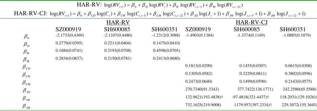
We include two single equation models of realized volatility in our forecast com-parison, which are the Heterogenous Autoregressive (HAR) model proposed by Corsi (2003), and an extension of this called a HAR-RV-CJ model proposed by Andersen, Bollerslev and Diebold (2007). Both models capture strong per-sistence in the volatility process by working with a lag structure that incorpor-ates past week and past month moving averages as predictors. The difference between the two specifications are that HAR models simply include predictors based on past realized volatility, whereas the HAR-RV-CJ models also include past week and past month bipower variation and jumps moving averages as predictors. The HAR-RV model islog(RVt+1) =β0+βDlog(RVt−1,t) +βWlog(RVt−5,t) +βMlog(RVt−22,t) +εt+1,
(15) whereRVt,t+h=h−1[RVt+1+RVt+2+...+RVt+h],forh= 5andh= 22,and the HAR-RV-CJ model is
log(RVt+1) = β0+βCDlog(Ct) +βCWlog(Ct−5,t) +βCMlog(Ct−22,t) (16)
whereCt,t+h=h−1[Ct+1+Ct+2+...+Ct+h]andJt,t+h=h−1[Jt+1+Jt+2+
...+Jt+h]forh= 5andh= 22.These models provide baselines for evaluating the various factor models outlined below. We include thefirst specification to determine forecast performance when a model is univariate and takes no ac-count of the different dynamic behavior of the continuous path variation and jumps, while the second allows the continuous and jump portions of past real-ized volatility to have separate effects on future realreal-ized volatility. We take the logarithms of each component when specifying the model, and then use
E(RVt+1|t) =exp(log(RVt+1|t) +
V ar(log(RVt+1|t))
2 )to obtain the one-step-ahead
realized volatility forecasting.
Table 4 shows the OLS regression results for the RV models and HAR-RV-CJ models for each of the three stocks. Comparing the R2 of those mod-els, we see that the R2 for the HAR-RV-CJ models are higher for each stock, (suggesting that the latter will forecast better), and since many of the jump coefficients are statistically significant for each stock, it appears that one will be able to exploit predictability in the jump component to make forecasting gains. This latterfinding is interesting, because the jump coefficients in the HAR-RV-CJ models of the US market in Andersen, Bollerslev and Diebold (2007) were statistically insignificant, and most of their gain in forecastability was due to their separation of the noise due to jumps from the continuous sample path.
4.2 Common Factor Models
We develop two sets of common factor models for total realized volatility and its bipower variation and jump components respectively, and then use various combinations of these models for forecasting in section 4.3.
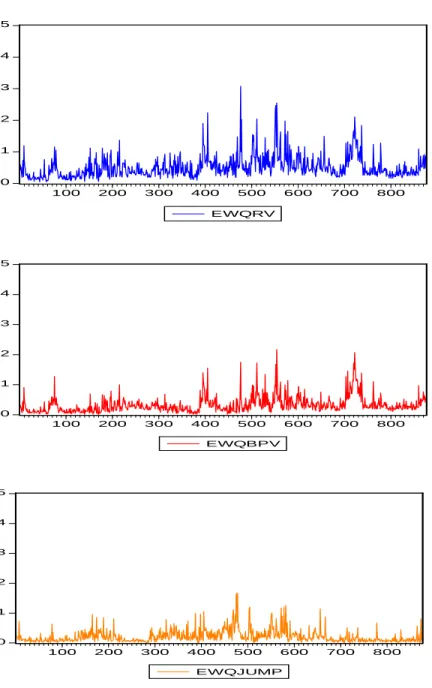
The first set of factor models simply take the equally weighted average of (i) the three log realized volatilities, (ii) the three log bipower variation series and (iii) three transformed jumps series9 as the estimated common factors for realized volatility, bi-power variation and jumps respectively. This method of determining estimates of common factors is motivated by the fact that if there is only one common factor in a multivariate series, then a simple average will provide a consistent estimate of it. The values of these equally weighted factors over the estimation sample are plotted in Figure 3 (after conversion back to levels), and not surprisingly they resemble the original series. Figure 3 shows that the (equally weighted) common factors of the continuous sample paths and jumps move differently from each other, which suggests that the two sources of variation are driven by different underlying factors. There is considerable interest in linking these underlying factors to fundamental macroeconomic vari-ables, (see Kim, Lee, Park and Yeo (2009)), but here our goal is to separately model the dynamic behavior of each of these factors so as to facilitate and improve forecasts.
For the equally weighted (EqW) factor models wefirstly calculate the
com-9We transform the jump series using ln(1 +J
t), since the presence of zeros precludes a
mon factors and thenfit them according to an ARMA(2,1) structure, where our choice of an ARMA(2,1) specification fulfills our need to capture long memory and provides a simple alternative to other long memory models such as AR-FIMA models. Next, we regress each of the three series on the factor to obtain factor loadings and the factor contribution to each of the three series. The re-maining idiosyncratic components are then modeled using ARMA terms, and AR(1) specifications seem to be sufficient in all cases. The resulting model of each trivariate realized volatility (bipower variation or jump) series is
⎛ ⎝ yy12 y3 ⎞ ⎠ = ⎛ ⎝ aa12 a3 ⎞ ⎠ft+et whereft=b1+b2ft−1+b3ft−2+b4vt−1+vt, (17) et = ⎛ ⎝ ee12tt e3t ⎞ ⎠= ⎛ ⎝ ρρ12eett−−12 ρ3et−3 ⎞ ⎠+ ⎛ ⎝ uu12tt u3t ⎞ ⎠,
vt ∼ i.i.d.N(0, σ2f) and ut(3×1)∼i.i.d.N(0(3×1), diag(σ21, σ22, σ23)(3×3)).
Apart from using a different transformation for the jump series, we undertake no further consideration of the fact that some of our raw jump observations were zero. The estimated coefficients are presented in Table 5. The estimated loading coefficients suggest that each stock makes approximately the same contribution to the realized volatility and bipower variation factors, although the second stock contributes relatively more to the former factors and relatively less to the jump factor. Theb2coefficients indicate that each factor is very persistent, but
as expected the persistence in the bi-power variation is higher than that in the jumps. Theb3andb4coefficients in the jump factor model are essentially zero,
so we impose this restriction for the jump factor. The estimatedρ coefficients range between 0.423 and 0.087, indicating that the factors themselves do not capture all of the persistence, but again we see that the persistence in the jumps is lower than that in bipower variation and realized volatility.
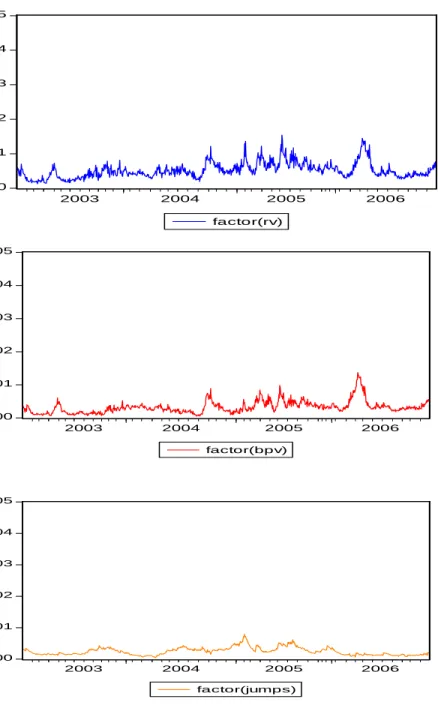
The second set of common factor models for the three components are state-space models that follow the same specification as above (i.e. equation 17), but now the factors, factor loadings and the processes for the idiosyncratic components are estimated simultaneously, and our jump model accounts for a jump variable (which is now defined by 10000×log(Jt+ 1)) that is only observed when it is greater than zero. We call these models state space (SSp) factor models, and present the estimated factors and coefficients in Figure 4 and Table 6 respectively. The estimated SSp common factors resemble the original series plotted in Figure 2 and the equally weighted factors plotted in Figure 3. The factor loading reported in Table 6 are quite similar to those in Table 5, but the persistence in the realized volatility and bipower variation factors is considerably lower. As before, theb3andb4coefficients in the jump factor model
are essentially zero, so we restrict the jump factor to be AR(1). Further, we find non-trivial persistence in the idiosynchratic components for all SSp models and model these as AR(1) processes.
cor-responding EqW model and then also forecast realized volatility using the sum of the implied predictions from the EqW model for bi-power variation and the EqW model for jumps (denoted by EqW(BV+J’), where the J’ indicates that estimation treats the zero observations as true zeros). Comparison of the former (i.e. EqW(RV)) model with univariate specifications provides information on whether the factor model offers an improvement, and comparison of the factor model for realized volatility with the composite factor model that combines in-formation from separate factor models for each of bipower variation and jumps allows us determine whether separate models of the components dominate a single model. We do the same for the SSp models (so that analogous compar-isons are possible), and also to see whether the special tobit type treatment of the transformed jump process offers an improvement. Finally, we re-estimate the jump factor model by casting it in state space form, but treating the zero observations as actual observations. This allows us to make further assessments of how different treatments of the problematic jump series affect forecasts.
We close this section with an in-sample forecasting exercise, which is under-taken to provide a comparison of how well each of the estimated modelsfits the data. Table 7 reports the in sample values of root mean squared error associ-ated with each model, and some results associassoci-ated with Giacomini and White (2006) tests of the null hypothesis that forecasting ability of two models is the same.10 Here, we see that the factor models always fit the data significantly better than the single equation representations, but that the separate model-ling of jumps is able to make a significant improvement with respect to fit in some, but not all cases. The "best model" in terms of in-sample root mean squared error is the EqW(BV+J’) model for two for the three stocks, although the difference between these models and the EqW(RV) model is statistically significant for only one of these stocks. While the SSp(BV+J) model has lower RMSE than the EqW(RV) model in two out of three cases, the SSp(BV+J) model has lower RMSE than the corresponding SSp(RV) in all three cases, and the difference is statistically significant for two out of the three stocks. Further the RSME for the SSp(BV+J) model for tone of the stocks (SH600351) is lower than that for all other models for that stock. The SSp(BV+J) models, which use the tobit type specification to deal with jump observations that are zero, fit slightly better than the SSp(BV+J’) models that directly use the observed zeros for estimation, although the difference is not large. This suggests that the tobit approach towards the factor modelling of jumps offers some potential for forecasting, although this potential might be limited.
4.3 Out-of Sample Forecast Comparison
We compare performance of the above described models with respect to out-or sample point realized volatility forecasting and quantile forecasting of the return
1 0The null hypothesis of this test is E(e2
1) = E(e22).This test is actually a t-test on the sample mean of(ee2
1−ee22)with a heteroskedasticity and autocorrelation consistent standard error.
distribution. Table 8 reports the RMSEs of all the models with respect to point forecasting of realized volatility. We can see that the multivariate common factor models always produce better forecasts than the univariate HAR type models, regardless of how the factors are modelled. The models in which continuous sample path and jumps are separately treated almost always provide better forecasts than models in which realized volatility is treated as a whole, in both univariate and multivariate settings. Overall, SSP(BPV+J) model offers the best forecasts for stock SZ000919 and stock SH600351, while the EqW(BPV+J’) model offers the best forecasts for stock SH600085. These results are consistent with the existing literature (see Anderson and Vahid (2007)) in that the mul-tivariate factor models outperform the univariate models in all three stocks. In addition, wefind that the separate factor modelling of the jump component of-fers improvement in RMSE. As before, we use the Giacomini and White (2006) test to determine whether the predictive superiority is significant or not, and we indicate statistically significant differences with asterisks. The tests indic-ate statistically significant improvements when comparing factor models with univariate models, but the improvements related to separate factor modelling of the jump component is only statistically significant for stock SZ000919. The relatively bad performance of SSP(BPV+J’) model in which the zeros in jump series are treated as if they were observed provides evidence that our Kalman filter modification is able to correct the estimation bias, and thereby improve the forecasting results of realized volatility.
We also explore the ability of our models to predict quantiles of the return distribution (Value-at-Risk (i.e. VaR)), which has been used in risk management as a downside risk measure. By using the forecasted realized volatility from our models into the return equationrt=μt+
q σ2RV t|t−1zt 11, we calculate VaR as V aRt|t−1 =μt|t−1+ q σRVt
|t−1Qα(z). We use the Angelidis and Degiannakis
(2006) VaR backtesting procedure12 to assess the risk predictive ability of our models. The mean square error (MSE) and mean absolute error (MAE) of all the models with respect to one-step-ahead VaR prediction with 1%, 5% and 10% significance level are reported in Table 9. We see that the models that separately treat bipower variation and jumps always provide better VaR forecasting than the direct models of total realized volatility, in both univariate and multivariate settings. The best VaR forecasting across different significance levels and differ-ent assets is always offered by our SSP(BPV+J) model, although we note that
1 1μ
t is the location (mean) of the distribution ofrt,
t
σ2RV
t|t−1 is the scale (standard deviation) of the distribution ofrtandztis a random variable, which is drawn from a specific
distribution with zero mean andσ2is an additional parameter that ensures that the rescaled innovation processzthas unit variance.
1 2The unconditional coverage test (Kupiec, 1995) and the independence test (Christofersen,
1998) are employed in thefirst stage to monitor the statistical adequacy of the VaR forecasts. These tests examine whether the average number of violations is statistically equal to the expected coverage rate and whether these violations are independently distributed. In the second stage, the loss function (Lopez, 1999) based on another risk measure called Expected Shortfall (ES) is used to rank each model’s predictive ability
the number of tail observations in our forecasting sample is small. Nevertheless, the improvement offered by treating jumps with special care is interesting and somewhat expected, because jumps form the principal constituent in the tails of return distributions, so that models in which jumps are treated explicitly are likely to help with respect to capturing the tail behavior.
5. Conclusion
In this paper, we extend the idea of separately modeling the continuous and jump components for realized volatility forecasting, from a univariate setting to a multivariate setting. As in Andersen et al (2007), wefind that the separate modelling of bi-power variation and jumps leads to improved forecasts, and as in Anderson and Vahid (2007) we find that it is useful to incorporate factor representations of the data. The first of these findings is easily understood once it is explicitly recognized that the continuous and jump components of realized volatility follow quite different dynamic processes, and the second can be attributed to the fact that parsimony (in this case obtained by incorporating factor modeling of each of the continuous and jump components) often leads to forecasting gains.
Our work in this paper focusses on building factor models of jumps that incorporate dynamics, and these can offer forecast potential if jumps are some-what predictable and account for a large proportion of realized volatility. Al-though jumps are sometimes calculated in a way that in theory exploits assumed unpredictability, in practice jump series may exhibit quite strong persistence, especially if the sampling frequency for realized volatility calculation has not fully accounted for the trade offbetween bias and efficiency. Further, in devel-oping stock markets such as the Chinese stock market studied here, jumps can account for up to thirty percent of the variation in realized volatility, so it can be beneficial to devote particular attention to the explicit modeling of jumps.
The fact that volatility jumps are non-negative necessitates the use of mod-els that are appropriate for such limited-dependent variables, and we deal with this problem in the multivariate context by proposing a dynamic tobit common factor model for jumps. We estimate this model by modifying the standard Kalmanfilter to correct the estimation bias incurred by zeros in jump series, and we believe that this sort of model has not been used in this or other applied contexts before. Our application to jump series can be criticized on the grounds that jumps and theln(1 +Jt)series are not well approximated by normal dis-tributions, although all that is really needed here is for the positive values of our jump series to resemble the right hand portion of a normal distribution. We then interpret our SSp jump process estimates as quasi-maximum likeli-hood estimates. An alternative approach might model the jumps using other assumptions about jump distributions. Such assumptions about distributions would, however, necessitate further adjustments to thefiltering process, and we leave this for further research.
con-tinuous and jump components of realized volatility offers forecasting gains, al-though the gain offered by our special treatment of the zeros in the jump series is not impressive. The gains are, however, seen with respect to both one step ahead point forecasts and one step ahead lower quantile forecasts of realized volatility, and some of these gains relative to factor models of realized volatility are statist-ically significant. Useful extensions of this work would include some analysis of forecasts based on rolling samples and forecasts over different horizons. Further, it would be useful to see if the factors associated with the continuous component of volatility could be related to underlyingfinancial/macroeconomic variables, or in the case of jumps, to news or announcements about the evolution of such variables.
Appendix A
State Space Model and the Kalman Filter (if
J
∗t
was
ob-served)
J
t∗=
αS
t+
u
t(18)
S
t=
β
1+
β
2S
t−1+
v
t(19)
Consider the state space model of (1) and (2) with normally distributed dis-turbancesut∼N(0, R)andυt∼N(0, Q). The recursive procedure tofind the optimal estimators of mean and variance of the distribution ofJt∗based on the available information up to timet−1is:
• Step 1 Prediction: From the initial stateS0|0, the optimal estimation of the
stateS1is made asS1|0 through equation (2) by using the information up
tot= 0. The covariance matrix of the estimation error can be calculated as P1|0. The optimal estimation of the observation J1∗ is made as J1∗|0
through the estimated stateS1|0and equation (1). The covariance matrix
of the estimation error can be calculated asG1|0.
S1|0=E(S1|I0) =β1+β2S0|0 P1|0=β2P0|0β 0 2+Q J1∗|0=αS1|0 G1|0=αP1|0α 0 +R
• Step 2 Updating: As the actual observation at timet= 1becomes avail-able, we can compare our prediction of J∗
1|0 with the observed values to
obtain the one-step-ahead prediction errore1|0. Although the actual state
S1 can not be observed, we can update the estimation of state vector as
S1|1 and the covariance matrix of the updated state asP1|1 based on the
new information at timet= 1. The updating mechanism is
e1|0=J1∗−J1∗|0 S1|1=S1|0+Cov(S1,J1∗|I0)V ar(J1∗|I0)−1e1|0=S1|0+P1|0α 0 G−1|10e1|0 P1|1=V ar(S1|I0)−Cov(S1,J1∗|I0)V ar(J1∗|I0)−1Cov(S1,J1∗|I0) 0 =P1|0−P1|0α 0 G1|0αP 0 1|0
• Step 3 Using the updated state vector and its updated covariance matrix, we can predict the measurement vector and its covariance matrix in next period by repeating steps 1 and 2. We keep repeating these steps until the final period, obtaining the one-step-ahead prediction errorset|t−1for each
period. The joint log likelihood function of {et|t−1}Tt=1can be written as
logL=−N T 2 log2π− 1 2 T X t=1 log|Gt|− 1 2 T X t=1 et0|t−1Gt−1et|t−1,
and the parameters can be estimated by maximizing this likelihood func-tion.
Appendix B
Moments of Multivariate Truncated Normal Distribution
This appendix is based on McGill (1992). Letφ(.;R) and Φ(.;R) denote the probability density function and the cumulative distribution function of ann -dimensional vector of standardized (i.e. mean zero and variance one) normal random variables with correlation matrixR.SupposeX is a multinormal ran-dom vector with mean vectorμ= (μ1,. . . , μn)0and variance-covariance mat-rixΣ. The joint density function ofX is:f(X;μ,Σ) = (2π)−n/2|Σ|−12exp{−1
2(X−μ)
0Σ−1(X
−μ)}=|S|−1φ(Z;R)
whereS2=diag(Σ),R=S−1ΣS−1andZ=S−1(X−μ).The associated joint
cumulative distribution function is:
F(X;μ,Σ) =
Z
(−∞,X]
f(X;μ,Σ)dX=Φ(Z;R)
where(−∞, X] = (−∞, x1]×(−∞, x2]× · · · ×(−∞, xn],anddX=dx1· · ·dxn. We want to deriveE(X|X < α)andV ar(X|X < α)whereα= (α1,···,αn)
0
is a given vector of constants. Following McGill (1992), we derive these by first deriving the moment generating function of a multivariate truncated nor-mal random variable and then using the moment generating function to derive the first two moments. By definition, the moment generating function of the truncated normal is:
M(t) = EX|X<α[exp(t 0 X)] = [Φ(S−1(α−μ);R)]−1 Z [−∞,α) (2π)−n/2|Σ|−12exp(−1 2[(X−μ) 0Σ−1(X −μ)−2t0X])dX = [Φ(S−1(α−μ);R)]−1Φ(S−1(α−μ−Σt);R) exp ½ t0μ+1 2t 0Σt ¾
By the properties of the moment generating function,
E(X |X < α) = ∂M(t) ∂t |t=0 V ar(X |X < α) = ∂ 2M(t) ∂t∂t0 |t=0−E(X|X < α)E(X |X < α) 0
Thefirst derivative of the moment generating function is:
∂M(t) ∂t = [Φ(S −1(α −μ);R)]−1exp ½ t0μ+1 2t 0Σt ¾ × £ −ΣS−1∇Φ(S−1(α−μ−Σt);R) + (μ+Σt)Φ(S−1(α−μ−Σt);R)¤
where∇Φ(S−1(α−μ−Σt);R)stands for then×1vector∂z∂ Φ(z;R)|z=S−1(α−μ−Σt). This implies E(X|X < α) = μ−ΣS−1∇Φ(S− 1(α−μ);R) Φ(S−1(α−μ);R) = μ−SR∇Φ(S− 1(α−μ);R) Φ(S−1(α−μ);R) .
The second derivative of the moment generating function is:
∂2M(t) ∂t∂t0 = ∂M(t) ∂t (μ+Σt) 0+ [Φ(S−1(α −μ);R)]−1exp ½ t0μ+1 2t 0Σt ¾ × £ ΣS−1∇2Φ(S−1(α−μ−Σt);R)S−1Σ+Φ(S−1(α−μ−Σt);R)Σ+ (μ+Σt)∇Φ(S−1(α−μ−Σt);R)0S−1Σ¤
Evaluating this att= 0and subtractingE(X |X < α)E(X|X < α)0leads to
V ar(X |X < α) =Σ+ΣS−1 ∙ ∇2Φ(z;R) Φ(z;R) − ∇Φ(z;R)∇Φ(z;R)0 Φ2(z;R) ¸ z=S−1(α−μ) S−1Σ.
By analogy with the univariate case, where the inverse Mills ratio is defined as the ratio of the PDF to the CDF of a random variable, we defineH(Z) = ∇ΦΦ((ZZ)). Then,
E(X |X < α) =μ−SRH(S−1(α−μ)),and
Appendix C
1.Moments of Multivariate Conditional Truncated Normal
Distribution
Suppose we have two random vectorsX and Y of dimensions NX and NY re-spectively, andX∼M N(μX,ΣX), Y ∼M N(μY,ΣY),andCov(X, Y) =ΣXY.
The transpose ofΣXY is denoted byΣY X.LetA= (−∞,0]NY.We want to de-riveE(X |Y ∈A)andV ar(X |Y ∈A)using the moment generating function ofX conditional on(Y ∈A).The conditional density ofX given(Y ∈A)is:
f(X|Y ∈A) =
R
ARf(X, Y)dY Af(Y)dY
.
1.1 Moment Generating Function The MGF is M(t) =E(et0X|Y ∈A) = Z (−∞,∞) et0X R ARf(X, Y)dY Af(Y)dY dX = [Φ(SY−1(0−μY);RY)]−1 Z A Z (−∞,∞) et0Xf(X, Y)dXdY = [Φ(SY−1(0−μY);RY)]−1 Z A EX|Y(et 0X )f(Y)dY = [Φ(SY−1(0−μY);RY)]−1 Z A (2π)−NY2 |ΣY| −1 2 et 0μ X|Y+12t 0Σ X|Yt.e−21(Y−μY)0Σ− 1 Y (Y−μY)dY = [Φ(SY−1(0−μY);RY)]−1et 0μ X+12t0ΣXt Z A (2π)−NY2 |ΣY|− 1 2 e− 1 2 (Y−μY−ΣY Xt) 0 Σ−1(Y−μY−ΣY Xt)dY = [Φ(S−Y1(0−μY);RY)]−1et 0μ X+12t0ΣXt[Φ(S−1 Y (0−μY −ΣY Xt);RY)] 1.2. Expected Value
Differentiating the MGF and evaluating it att= 0leads to:
E(X|Y ∈ A) =∂M(t) ∂t |t=0=μX−ΣXYS −1 Y ∇ Φ(SY−1(0−μY);RY) Φ(S−Y1(0−μY);RY) = μX−ΣXYSY−1H¡SY−1(0−μY)¢.
Using the fact thatSY−1H¡SY−1(0−μY)¢=−Σ−Y1(E(Y |Y ∈A)−μY), we can rewrite the above as:
E(X|Y ∈A) =μX+ΣXYΣY−1(E(Y |Y ∈A)−μY),
which is a result that could be derived directly using the linearity of the condi-tional expectation function of normally distributed random variables..
1.3 Variance We know that: V ar(X|Y ∈ A) =E(XX0|Y ∈A)−E(X|Y ∈A)E(X|Y ∈A)0 = ∂ 2M(t) ∂t∂t0 |t=0−E(X|Y ∈A)E(X|Y ∈A)0 and E(XX0|Y ∈ A) =∂ 2M(t) ∂t∂t0 |t=0=ΣX+μXμ0X− 2μX∇Φ(S −1 Y (0−μY);RY)0 Φ(SY−1(0−μY);RY) SY−1ΣY X+ΣXYSY−1[∇ 2 Φ(SY−1(0−μY);RY) Φ(SY−1(0−μY);RY) ]SY−1ΣY X. These lead to V ar(X|Y ∈A) =ΣX+ΣXYSY−1∇[H(SY−1(0−μY)]SY−1ΣY X
Since∇(H(SY−1(0−μY)) = (SYRY)−1(ΣY −V ar(Y|Y ∈A))(SYRY)−1,13 the variance expression can be transformed to:
V ar(X|Y ∈A) =ΣX−ΣXYΣ−Y1(ΣY −V ar(Y|Y ∈A))Σ−Y1ΣY X
2. Moments of Multivariate Conditional Mixed Truncated
Normal and Normal Distribution
Suppose we have three normally distributed vectors X, Y and Z, where X ∼ M N(μX,ΣX) , Y ∼ M N(μY,ΣY), and Z ∼ M N(μZ,ΣZ), and let ΣU V de-note covariance between random vectors U and V with ΣV U = Σ0
U V. Let
A= (−∞,0]NY. We want to derive theE(X|Y ∈A, Z)andV ar(X|Y ∈A, Z) using the moment generating function of X conditional on (Y ∈A, Z). The conditional density ofX given(Y ∈A, Z)is:
f(X|Y ∈A, Z) =
R
ARf(X, Y|Z)dY Af(Y|Z)dY
.
2.1. Moment Generating Function The MGF is M(t) =E(et0X|Y ∈A, Z) = Z (−∞,∞) R (−∞,0]e t0Xf(X, Y |Z)dY R (−∞,0]f(Y|Z)dY dX = [Φ(SY−|1Z(0−μY|Z);RY|Z)]−1 Z (−∞,0] ( Z (−∞,∞) et0Xf(X|Y, Z)dX).f(Y|Z)dY
= [Φ(SY−1|Z(0−μY|Z);RY|Z)]−1 Z (−∞,0) EX|Y,Z(et 0X ).f(Y|Z)dY = [Φ(SY−|1Z(0−μY|Z);RY|Z)]−1 1 |ΣY|Z| (2π)−NY2 Z (−∞,0) et0uX|Y,Z+12t0ΣX|Y,Zt·e− 1 2 (Y−uY|Z)0ΣY−1|Z(Y−uY|Z) dY = [Φ(SY−|1Z(0−μY|Z);RY|Z)]−1et 0μ X|Z+12t0ΣX|Zt[Φ(S−1 Y|Z(0−μY|Z−ΣXY|Zt);RY|Z)] 2.2 Expected Value By definition: E(X|Y ∈A, Z) = ∂M(t) ∂t |t=0=μX|Z−ΣXY|ZS −1 Y|Z ∇Φ(SY−1|Z(0−μY|Z);RY|Z) Φ(SY−|1Z(0−μY|Z);RY|Z) Since E(X|Y ∈A, Z) =μX|Z+ΣXY|ZSY−|1Z(SY|ZRY|Z)−1(E(Y|Y ∈A, Z)−μY|Z) =μX|Z+ΣXY|ZΣ−Y1|Z(E(Y|Y ∈A, Z)−μY|Z) =μX+ΣX,(Y,Z)Σ−(Y,Z1 )( E(Y|Y ∈A, Z)−μY Z−μZ )
which could be derived directly given the linearity of the conditional expectation function. 2.3 Variance By definition, V ar(X|Y ∈A, Z) =E(XX0|Y ∈A, Z)−E(X|Y ∈A, Z)E(X|Y ∈A, Z)0 =ΣX|Z−ΣXY|ZSY−1|Z∇[H(SY−1|Z(0−μY|Z)] 0 SY−1 |ZΣY X|Z where E(XX0|Y ∈A) = ∂ 2M(t) ∂t∂t0 |t=0 =ΣX|Z+μX|Zμ0X|Z−2μX|Z ∇Φ(SY−|1Z(0−μY|Z);RY|Z)0 Φ(SY−|1Z(0−μY|Z);RY|Z) SY−1 |ZΣY X|Z +SY−1 |ZΣX,Y|Z[ ∇2Φ(S−Y|1Z(0−μY|Z);RY|Z) Φ(SY−1|Z(0−μY|Z);RY|Z) ]SY−1 |ZΣX,Y|Z Since ∇(H(SY−1 |Z(0−μY|Z) = (SY|ZRY|Z)−1(ΣY|Z−V ar(Y|Y ∈A, Z))(SY|ZRY|Z)−1,
the variance expression can be transformed to:
V ar(X|Y ∈A, Z) =ΣX|Z−ΣXY|ZΣ−Y1|Z(ΣY|Z−V ar(Y|Y ∈A, Z))Σ−Y1|ZΣY X|Z
=ΣX−ΣX(Y,Z)Σ−(Y,Z1 )Σ
M
(Y,Z)Σ−(Y,Z1 )Σ(Y,Z)X Where ΣM (Y,Z)= ∙ ΣY −V ar(Y|Y ∈A, Z) ΣY Z−Cov(Y, Z|Y ∈A, Z) ΣY Z−Cov(Y, Z|Y ∈A, Z) ΣZ ¸ , V ar(Y|Y ∈A) =ΣY −SYRY∇(H(−S−1(0−μY)))0RYSY, and Cov(Y, Z|Y ∈A) =ΣY Z−SY ZRY Z∇(H(−SY−1(0−μY)))0RY ZSY Z..