Estimation for the change point of volatility in a stochastic differential equation

(1)

and sharing with colleagues.

Other uses, including reproduction and distribution, or selling or licensing copies, or posting to personal, institutional or third party

websites are prohibited.

In most cases authors are permitted to post their version of the article (e.g. in Word or Tex form) to their personal website or institutional repository. Authors requiring further information

regarding Elsevier’s archiving and manuscript policies are encouraged to visit:

(2)

Stochastic Processes and their Applications 122 (2012) 1068–1092

www.elsevier.com/locate/spa

Estimation for the change point of volatility in a

stochastic differential equation

✩

Stefano M. Iacus

a,∗

_{, Nakahiro Yoshida}

b,c

a_{Department of Economics, Business and Statistics, University of Milan, Via Conservatorio 7, 20122 Milan, Italy} b_{University of Tokyo, Japan}

c_{Japan Science and Technology Agency Graduate School of Mathematical Sciences, University of Tokyo, 3-8-1} Komaba, Meguro-ku, Tokyo 153-8914, Japan

Received 27 December 2010; received in revised form 15 November 2011; accepted 15 November 2011 Available online 1 December 2011

Abstract

We consider a multidimensional Itˆo process Y = (Y_t)_t_∈[₀_,_T_] with some unknown drift coefficient

processbt and volatility coefficientσ(Xt, θ)with covariate processX =(X_t)_t_∈[₀_,_T_], the functionσ (x, θ)

being known up to θ ∈ Θ. For this model, we consider a change point problem for the parameter θ in

the volatility component. The change is supposed to occur at some pointt∗ _∈ ₍₀_,_T₎_{. Given discrete time} observations from the process (X,Y), we propose quasi-maximum likelihood estimation of the change point. We present the rate of convergence of the change point estimator and the limit theorems of the asymptotically mixed type.

c

Keywords:Itˆo processes; Discrete time observations; Change point estimation; Volatility

1. Introduction

The problem of change point has been considered initially in the framework of independent and identically distributed data by many authors, see e.g. [9,7,5,13]. Recently, it naturally moved to context of time series analysis, see for example, [15,18,3] and the papers cited therein.

✩_{This work was in part supported by the JST Basic Research Programs PRESTO, Grants-in-Aid for Scientific}

Research No. 19340021, the Global COE program “The research and training center for new development in mathematics” of Graduate School of Mathematical Sciences, University of Tokyo, and by the Cooperative Research Program of the Institute of Statistical Mathematics.

∗_{Corresponding author.}

(3)

In fact, change point problems have originally arisen in the context of quality control, but the problem of abrupt changes in general arises in many contexts like epidemiology, rhythm analysis in electrocardiograms, seismic signal processing, study of archaeological sites and financial markets. In particular, in the analysis of financial time series, the knowledge of the change in the volatility structure of the process under consideration is of a certain interest.

In this paper we deal with a change-point problem for the volatility of a process solution to a stochastic differential equation, when observations are collected at discrete times. The instant of the change in volatility regime is identified retrospectively by maximum likelihood method on the approximated likelihood. For continuous time observations of diffusion processes [19] considered the change point estimation problem for the drift. In the present work we only assume regularity conditions on the drift process. De Gregorio and Iacus [6] considered a least squares approach following the lines of [1,2] of a simplified model also under discrete sampling while [22] considered a CUSUM approach. Finally it should be noted that the problems of the change-point for the drift function of ergodic diffusion processes have been treated by Kutoyants [16,17], however the asymptotic results and the sampling schemes are different from this paper. Notice also that, as usual in change point problems, due to non smoothness of the statistical model with respect to the parameter to be estimated (the change point instant), the rate of convergence of the change point estimator is faster than usual rate of estimators in regular models [12].

The paper is organized as follows. Section 2 introduces the model of observation, the regularity conditions and some notation. We shall treat two asymptotic settings: there are two models before and after the change point. In one case (A) the two models remain distinct in the limit (fixed alternatives), in the second case (B) they get closer and closer (contiguous alternatives, see [20]). Section 3 studies consistency and the rate of convergence of estimator of the change while asymptotic distributions are considered in Section 4. A mixture of certain Wiener functionals appears as the limit of the likelihood ratio random field, and it characterizes the limit distribution of the change-point estimator. Those sections assume that consistent estimators of the volatility parameters are available. Section5contains a preliminary interesting inequality which is used to study the asymptotic distribution of the change point estimator in case (A). Section 6 presents some practical considerations and a proposal to obtain first stage estimators of the volatility parameters which allow to obtain all asymptotic properties stated in the previous sections. Finally, Section 7 presents some numerical analysis to assess the performance of the estimators.

2. Estimator for the change-point of the volatility

Consider a d-dimensional Itˆo process Y = (Y_t)_t_∈[₀_,_T_] satisfying the stochastic differential

equation

dYt =b_tdt+σ(X_t, θ)dW_t, t ∈ [0,T]

on a probability space, where Wt is anr-dimensional standard Wiener process, on a stochastic

basis,bt andXt are vector valued progressively measurable processes, andσ (x, θ): X ×Θ → Rd ⊗Rr is a matrix valued function.

We assume that there is the time t∗ _{across which the diffusion coefficient changes from}

σ (x, θ0) to σ(x, θ1). The change point t∗ ∈ (0,T) is unknown and we want to estimate t∗

(4)

to be known up to the parameterθ, whilebt is completely unknown and unobservable, therefore

possibly depending onθ andt∗_.

The sample consists of (Xti,Yti), i = 0,1, . . . ,n, where ti = ih for h = hn = T/n. The

parameter spaceΘ of θ is a bounded domain inRd0,d₀ ≥ 1, and the parameterθ is a nuisance

in estimation oft∗_{. Denote by}_θ∗

i the true value ofθi fori = 0,1.

Letϑn = |θ₁∗−θ₀∗|. We will consider the following two different situations.

(A) θ∗

0 andθ1∗ are fixed and do not depend onn.

(B) θ∗

0 andθ1∗ depend onn, and asn → ∞,θ0∗ → θ∗ ∈Θ,ϑn →0 andnϑn2 → ∞.

In Case (A),ϑn is a constantϑ0independent ofn.

We shall formulate the problem more precisely. It will be assumed that the process Y

generating the data is an Itˆo process realized on a stochastic basis B = (Ω,F,F,P) with

filtrationF =(F_t)_t_∈[₀_,_T_], and satisfies the stochastic integral equation

Yt =        Y0+  t 0 bsds +  t 0 σ (Xs, θ ∗ 0)dWs fort ∈ [0,t∗) Yt∗ +  t t∗ bsds +  t t∗ σ (Xs, θ ∗ 1)dWs fort ∈ [t∗,T].

HereWt is anr-dimensionalF-Wiener process onB, andbt,Xt andσ (x, θ)satisfy the conditions

below. Let X be a set in Rd1 (possibly X ₌ Rd1) and denote the modulus of continuity of a

function f : I →Rd1 by

wI(δ, f)= sup

s,t∈I,|s−t|≤δ

|f(s)− f(t)|.

For matrices M = (m_{i j}) and N = (n_{i j}) of the same size, we write M⊗2 = MtM, M[N] = 

i j mi jni j = Tr(MtN), and the Euclidean norm of M by|M| = (M[M])1/2. Set S(x, θ) =

σ (x, θ)⊗2_._λ

1(M)denotes the minimum eigenvalue of a symmetric matrix M. Let us denote by ∂_θℓf the partial derivative of orderℓof function f with respect toθ. Letαbe a positive number.

[H]_j (i) σ(x, θ)is a measurable function defined onX ×Θ satisfying

(a) inf(x,θ)∈X×Θλ1(S(x, θ)) >0,

(b) derivatives ∂_θℓσ (0 ≤ ℓ ≤ j + [d₀/2]) exist and those functions are continuous on

X ×Θ,

(c) there exists a locally bounded function L :X ×X ×Θ →R+such that

|σ(x, θ)−σ (x′, θ)| ≤ L(x,x′, θ)|x −x′|α (x,x′∈X, θ ∈Θ).

(ii)(Xt)t∈[0,T] is a progressively measurable process taking values inX such that

w[0,T] 1 n,X  = o_p(ϑ_n1/α) asn → ∞.

(iii) (bt)t∈[0,T] is a progressively measurable process taking values in Rd such that

(bt −b₀)_t_∈[₀_,_T_]is locally bounded.

Remark 1. The term “locally bounded” in[H]_j (i) (c) means, as usual, being bounded on every

compact set, i.e.bt is locally bounded if there exists a sequence of increasing stopping timessn

such thatbsn∧t is bounded. The case where the drift bt changes its structure at time t∗, or any

time in force, is included in our context becausebt admits jumps. The case of time dependentσ is

(5)

to say, if we set X or a part of X as Y, then our model can express a system with feedback, in particular, a diffusion process. By[H]_j (ii),t → X_t is continuous a.s. Also,[H]_j (ii) imposes a

restriction on the rateϑn. For example, whenα = 1, for a Brownian motion X, it suffices that

nϑ2

n/logn → ∞, due to L´evy property. The additional [d0/2]time differentiability to j is used

only in Step (iii) of the proof of Theorem 1. If one can introduce a different set of conditions that ensures the H´ajek–Renyi type estimate before making use of inequality(4)below, then it is possible to limit the range ofℓfrom “0 ≤ℓ≤ j + [d₀/2]” to “0≤ ℓ≤ j”.

Write∆iY = Y_t_i −Y_t_i₋₁ and let

Φn(t;θ₀, θ₁)= [nt/T]  i=1 Gi(θ0)+ n  i=[nt/T]+1 Gi(θ1), where Gi(θ) = log detS(X_t_i₋₁, θ)+h−1S(X_t_i₋₁, θ)−1[(∆_iY)⊗2].

Suppose that there exists an estimator _θˆ_k _{for each} _θ∗

k, k = 0,1. Each estimator is based on

(Xti,Yti)i=0,1,...,n and so depends on n. See Section 6 for some discussion on how to obtain

consistent estimators_θˆ_k_,_k ₌ ₀_,_{1. To make our discussion complete, in case}_θ∗

k are known, we

define_θˆ

k just asθˆk =θ_k∗. This article proposes ˆ

tn = argmin

t∈[0,T]

Φn(t; ˆθ₀,θˆ₁)

for the estimation oft∗_{. More precisely,}_t_ˆ

n is any measurable function of(Xti)i=0,1,...,nsatisfying

Φn(tˆn; ˆθ₀,θˆ₁)= min

t∈[0,T]Φn(t

; ˆθ₀,θˆ₁).

Remark that our quasi-likelihood approach generalizes previously proposed methods, see e.g. [8], to the case of stochastic regression models with coordinates(Yt,Xt).

3. Rate of convergence

We introduce identifiability conditions in order to ensure consistent estimation. In Case (A) we assume [A] P S(Xt∗;θ∗ 0)̸= S(Xt∗;θ∗ 1)  =1; In Case (B) we assume

[B] Ξ(Xt∗, θ∗)is positive-definite a.s., where

Ξ(x, θ)= Tr((∂_θ₍_i₁₎S)S−1(∂_θ₍_i₂₎S)S−1)(x, θ)d0

i1,i2=1, θ

= (θ(i)).

Remark 2. SinceΞ(x, θ∗₎_{is the Hessian matrix of the nonnegative function}

Q(x, θ∗_{, θ)} := Tr  S(x, θ∗₎−1_S₍_x_{, θ)} − I_d  −log det  S(x, θ∗₎−1_S₍_x_{, θ)} ofθ atθ∗_,_Ξ₍_x_{, θ}∗₎_{is nonnegative-definite.}

The following property will be necessary to validate our estimating procedure. [C] | ˆθ_k −θ_k∗| =o_p(ϑ_n)asn → ∞fork =0,1.

(6)

In case the parameters are known,_θˆ

k should readθ_k∗, and then Condition [C] requires nothing.

Section6presents an example of estimator forθk which satisfies Condition [C].

Here we state the result on the rate of convergence of our change-point estimator.

Theorem 1. The family{nϑ_n2(tˆ_n −t∗)}_n_∈_N is tight under any one of the following conditions.

(a) [H]₁,[A]and[C]hold in Case(A).

(b) [H]₂,[B]and[C]hold in Case(B).

In both Case (A) and (B) this result gives consistency oftˆ_n, sincenϑ2

n → ∞by assumption,

which is true also in Case (B).

The rest of this section will be devoted to the proof of Theorem 1. Define a stopping time

τ = τ(K)by

τ(K)= inf{t; |X_t| + |b_t| > K} ∧T

for K > 0. Xτ _{denotes the process} _X _{stopped at} _τ_{. Write} _S_i_(θ) ₌ _S₍_Xτ

ti, θ), and ∆iYτ = Y_tτ_i −Y_tτ i−1. Let Ψn(t;θ₀, θ₁)= [nt/T]  i=1 gi(θ0)+ n  i=[nt/T]+1 gi(θ1), where gi(θ) = 1{τ>0}  log detSi−1(θ)+h−1Si−1(θ)−1[(∆iYτ)⊗2]  = 1_{_τ>₀_}log detS_i₋₁(θ)+h−1S_i₋₁(θ)−1[(∆_iYτ)⊗2]. Then sup_θ∈K|gi(θ)| ∈ L ∞− _{= ∩}

p>1Lp for any compact set K in Θ under [H]1. Denote by

Eθ1∗

i−1 the conditional expectation with respect toFti−1 under the true distribution forti−1 ≥t

∗_. Lemma 1. For t > t∗_, Ψn(t;θ₀, θ₁)−Ψ_n(t∗;θ₀, θ₁)= M_n(t;θ₀, θ₁)+ A_n(t;θ₀, θ₁)+ρ_n(t;θ₀, θ₁), where Mn(t;θ₀, θ₁)= [nt/T]  i=[nt∗_/_T_]+₁  [g_i(θ₀)−g_i(θ₁)] −Eθ ∗ 1 i−1[gi(θ0)−gi(θ1)]  , An(t;θ₀, θ₁) = 1_{_τ>₀_} [nt/T]  i=[nt∗_/_T_]+₁  TrSi−1(θ0)−1Si−1(θ1)− Id  − log det  Si−1(θ0)−1Si−1(θ1)  , ρn(t;θ₀, θ₁) = 1_{_τ>₀_} [nt/T]  i=[nt∗_/_T_]+₁ Tr Si−1(θ1)−1− Si−1(θ0)−1  ·  Si−1(θ1)−h−1E θ∗ 1 i−1[(∆iYτ) ⊗2_]_.

(7)

Remark 3. Later we will consider substitution of estimators _θˆ_k _to _θ_k_, _k ₌ ₀_,_{1. Then the}

expectation Eθ1∗

i−1[gi(θ0)−gi(θ1)]is taken before the substitution, and so

Mn(t; ˆθ₀,θˆ₁)= [nt/T]  i=[nt∗_/_T_]+₁  [g_i(θˆ₀)−g_i(θˆ₁)] −Eθ ∗ 1 i−1[gi(θ0)−gi(θ1)]|θ₀= ˆθ₀,θ₁= ˆθ₁  .

In particular, the second term in the braces is not necessarilyFti−1-measurable.

We will need a uniform H´ajek–Renyi inequality. Let D be a bounded open set in Rd. The Sobolev norm is denoted by

∥f∥_s_,_p =  s  i=0 ∥∂_θi f∥_Lp_p₍_D₎ 1/p

for f ∈Ws,p(D), the Sobolev space with indices(s,p). Suppose that p > 1 ands > d/p. The

embedding inequality is the following sup

θ∈D

|f(θ)| ≤ C∥f∥_s_,_p (f ∈ Ws,p(D)) (1)

where C is a constant depending only on s, p and D. We will apply this inequality for

f ∈ Cs(D), and the validity of such an inequality depends on the regularity of the boundary of

D; the Garsia–Rodemich–Rumsey (GRR) inequality validates it if there exist positive numbers

a andϵ0 such that

inf

θ∈Dν(Bϵ(θ))

≥aϵd forϵ ∈(0, ϵ₀), (2)

where ν is the Lebesgue measure on D and Bϵ(θ) is theϵ-ball centered atθ, see e.g. [24] for

details.

Lemma 2. Let(Ω,F,F = (F_j)_j_∈_Z+,P)be a stochastic basis. Let D be a bounded domain in Rd _{admitting Sobolev’s inequality}₍₁₎_{for some p} _∈ ₍₁_,₂_]_{and s} _∈ _Z₊ _{such that s} _> _d_/_{p. Let}

(cj)j∈Z+ be a nondecreasing sequence of positive numbers. Let X =(Xj)j∈Z+ be a sequence of

random fields on D for j ∈Z₊ satisfying the following conditions:

(i) For each(w, j)∈Ω ×Z₊, X_j ∈Cs(D);

(ii) For each (θ,i) ∈ D × {0,1, . . . ,s}, (∂_θiX_j(θ))_j_∈_Z₊ is a zero-mean Lp-martingale with

respect toF.

Then there exists a constant C′_{depending only on s}_, _{p and D, not depending on X, such that}

P  max j≤n 1 cj supD |X_j(θ)| ≥a  ≤ C ′ ap n  j=0 1 cp_j E  ∥X_j − X_j₋₁∥_sp_,_p

for all a >0and n ∈Z₊.

Proof. Let B = Lp(D), then B is p-uniformly smooth; see Definition 2.2 of [23, pp. 245–246,

and Example 2.2, p. 247]. We apply Theorem in [21, p. 245], to conclude

P  max j≤n 1 cj ∥∂_θiX_j∥_B ≥a  ≤ C1 ap n  j=0 1 cp_j E  ∥∂_θiX_j −∂_θiX_j₋₁∥p_B 

(8)

Proof of Theorem 1. For the proof, we may assume T = 1 for notational simplicity without

loss of generality.

(i) Letϵ be an arbitrary positive number. Set

H(x)= 4Q(x, θ₀∗, θ₁∗)ϑ₀−2

in Case (A), and set H(x) = λ₁(Ξ(x, θ∗)) in Case (B). We denote σ (t;θ) = σ (X_tτ, θ) and

h(t)= H(X_tτ)in what follows. Those processes depend onK by definition while it is suppressed

from the symbols. SetBK = {τ =1}and fix a sufficiently largeK so that P[B_Kc ]< ϵ/4.

We notice that h(s) ≥ 0 and that h(t∗) > 0 a.s. on B_K from the identifiability condition

[A]/[B] since Xτ_t∗ = Xt∗ onBK. We will show that there exists a positive constantcϵ such that

P  inf t∈[t∗_,₁_] 1 t −t∗  t t∗ h(s)ds ≤5c_ϵ  < ϵ.

Define the eventAδ by

Aδ =  inf t∈[t∗_,_t∗₊_δ_]h(s)≥ 1 2h(t ∗₎ 

forδ ∈(0,1−t∗). OnA_δ, it holds that

inf t∈[t∗,t∗+δ] 1 t −t∗  t t∗ h(s)ds ≥ 1 2h(t ∗ )≥ δ 2(1−t∗)h(t ∗ )

and also that, fort ∈ [t∗+δ,1],

1 t −t∗  t t∗ h(s)ds ≥ 1 1−t∗  t t∗ h(s)ds ≥ 1 1−t∗  t∗+δ t∗ h(s)ds ≥ δ 2(1−t∗)h(t ∗_).

Choose aδso that P[A_δ]> 1−ϵ/2 by the continuity ofh, and next choose a positive number

cϵ = c(ϵ, δ)such that P  δ 2(1−t∗)h(t ∗_{) >}₅_c ϵ  ≥ P  δ 2(1−t∗)h(t ∗_{) >}₅_c ϵ   BK  >1− ϵ 2. Then P  inf t∈[t∗_,₁_] 1 t −t∗  t t∗ h(s)ds ≤5c_ϵ  ≤ P[Ac_δ] +P  Aδ, inf t∈[t∗_,₁_] 1 t −t∗  t t∗ h(s)ds ≤5c_ϵ  < ϵ.

(ii) WithLemma 1, we decomposeΨn(t; ˆθ₀,θˆ₁)−Ψ_n(t∗; ˆθ₀,θˆ₁)as follows:

(9)

Let M ≥1. We have P[nϑ_n2(tˆ_n −t∗) > M] ≤ P  inf t:nϑ_n2(t−t∗_)>_MΦn(t ; ˆθ₀,θˆ₁)≤Φ_n(t∗; ˆθ₀,θˆ₁)  ≤ P  inf t:nϑ_n2(t−t∗_)>_MΨn(t ; ˆθ₀,θˆ₁)≤Ψ_n(t∗; ˆθ₀,θˆ₁)  +P[Bc_K]< P₁_,_n + P₂_,_n + P₃_,_n+ϵ, (3) where P1,n = P  sup t:nϑ_n2(t−t∗_)>_M 1 [nt] − [nt∗_]   Mn(t; ˆθ0, ˆ θ1)   ≥ cϵϑn2 3  P2,n = P  inf t:nϑ_n2(t−t∗_)>_M 1 [nt] − [nt∗_]An(t; ˆθ0, ˆ θ1)≤c_ϵϑ_n2  P3,n = P  sup t:nϑ_n2(t−t∗_)>_M 1 [nt] − [nt∗_]   ρn(t; ˆθ0, ˆ θ1)   ≥ cϵϑ_n2 3  .

Here we read inf∅ = ∞and sup∅ = −∞. We will estimate these terms.

(iii) Estimate of P1,n. In Case (B), let Mn(t;θ)= [nt]  i=[nt∗_]+₁  ∂θgi(θ)− Eθ ∗ 1 i−1[∂θgi(θ)]  .

Let_Θ˙ _{be an open ball such that}_θ∗ _{∈ ˙}_Θ _and_Θ_˙ _⊂ _Θ_{. Since}

By the uniform version of the H´ajek–Renyi inequality inLemma 2applied to the case p =2,

s =2+ [d₀/2]and D = ˙Θ, we see under[H]₂ that

P  sup t:nϑ_n2(t−t∗_)>_M 1 [nt] − [nt∗_] sup θ∈ ˙Θ |M_n(t;θ)| ≥ cϵϑn 6  ≤ C c2 ϵM =: ρϵ(M),

whereCdenotes a generic constant independent ofnand M. Therefore lim

(10)

thanks to P| ˆθ₀− ˆθ₁| ≥2ϑ_n  ≤ P  | ˆθ₀−θ₀∗| ≥ 1 3ϑn  + P  | ˆθ₁ −θ₁∗| ≥ 1 3ϑn  for largen.

In Case (A), Let_Θ˙

k be an open ball such thatΘ˙k ⊂ Θ andθ_k∗ ∈ ˙Θ_k for eachk = 0,1.

P1,n ≤ P    sup t:nϑ₀2(t−t∗_)>_M 1 [nt] − [nt∗_] sup θ₀∈ ˙Θ₀ θ₁∈ ˙Θ₁ |M_n(t;θ₀, θ₁)| ≥ cϵϑ 2 0 3    +P[ ˆθ₀ ̸∈ ˙Θ₀] + P[ ˆθ₁ ̸∈ ˙Θ₁].

We apply the H´ajek–Renyi inequality for Mn(t;θ₀, θ₁), which is a difference of two random

fields on_Θ˙

k to be done with one by one, in order to obtain(4)under[H]₁.

(iv) Estimation of P2,n. First we consider Case (B). There is a positive constant c2 independent

ofn such that TrSi−1(θˆ0)−1Si−1(θˆ1)− Id  −log det  Si−1(θˆ0)−1Si−1(θˆ1)  ≥Ξ(X_tτ i−1, θ ∗₎ [(θˆ₁− ˆθ₀)⊗2] +r_n_,_i−1| ˆθ1− ˆθ0|2 ≥ {λ₁(Ξ(Xτ_t i−1, θ ∗ ))+r_n_,_i₋₁}| ˆθ₁− ˆθ₀|2

for alli, where maxi|r_n_,_i₋₁| ≤ c₂ϑ_n, on the event

BK,n = B_K ∩ { ˆθ₀,θˆ₁ ∈ ˙Θ,| ˆθ_k −θ∗| ≤ϑ_n(k = 0,1)}. Thus P2,n ≤ P  inf t:nϑ_n2(t−t∗_)>_M 1 [nt] − [nt∗]An(t; ˆθ0, ˆ θ1)| ˆθ₁− ˆθ₀|−2 ≤4c_ϵ,B_K_,_n  +P  | ˆθ₁− ˆθ₀| ≤ 1 2ϑn  + P[B_Kc_,_n] ≤ P  inf t:nϑ_n2(t−t∗_)>_M 1 [nt] − [nt∗_] [nt]  i=[nt∗_]+₁ {λ₁(Ξ(X_tτ i−1, θ ∗₎₎₊_r n,i−1} ≤4cϵ  +ϵ

for largen. The scaled summation converges to the corresponding scaled integral uniformly int

a.s., hence from Step (i) we have lim n→∞P2,n ≤ P  inf t∈[t∗_,₁_] 1 t −t∗  t t∗ h(s)ds ≤5c_ϵ  +ϵ <2ϵ for largen.

We will consider Case (A). There is a positive constantc2 independent ofnsuch that

TrSi−1(θˆ0)−1Si−1(θˆ1)− Id  −log det  Si−1(θˆ0)−1Si−1(θˆ1)  ≥Tr  Si−1(θ₀∗)−1Si−1(θ₁∗)− Id  −log det  Si−1(θ₀∗)−1Si−1(θ₁∗)  −c₂(| ˆθ₁−θ₁∗| + | ˆθ₀−θ₀∗|)

(11)

for all i on the event B′

K,n = BK ∩ { ˆθ0 ∈ Θ˙0,θˆ1 ∈ Θ˙1} because there exists a continuous

derivative∂θσ by[H]₁. In this way,

P2,n ≤ P  inf t:n(t−t∗_)>_M 1 [nt] − [nt∗_]An(t; ˆθ0, ˆ θ1)≤c_ϵϑ₀2,B′_K_,_n  + PB′_Kc_,_n. Therefore, lim n→∞P2,n ≤ P  inf t∈[t∗_,₁_] 1 t −t∗  t t∗ h(s)ds ≤5c_ϵ  +ϵ <2ϵ by Step (i). (v) Estimation of P3,n. We have sup t∈[t∗_,₁_]   S(Xt, ˆ θk)− S(X_t, θ_k∗)    1{| ˆθ_k−θ_k∗|<2ϑ_n}∩B_K ≤Cϑn (k = 0,1), sup t∈[t∗,1]   S(Xt, ˆ θk)−1− S(X_t, θ_k∗)−1    1{| ˆθ_k−θ_k∗|<2ϑ_n}∩B_K ≤Cϑn (k =0,1) and sup i:≥[nt∗_]+₂   Si−1(θ ∗ 1)−h−1Eθ ∗ 1 i−1[(∆iY) ⊗2 ]   1BK ≤Cw[0,T]  X, 1 n α .

In the last estimate, the local α-H¨older continuity ofσ was used. Then on BK ∩ {| ˆθ_k −θ_k∗| ≤

2ϑn(k = 0,1)}, sup t:nϑ_n2(t−t∗_)>_M 1 [nt] − [nt∗_]   ρn(t; ˆθ0, ˆ θ1)   ϑ −2 n = op(1) (5)

because of [H]_j (ii). Consequently, we see lim_n_→∞P₃_,_n ≤ ϵ due to [C] and the localization

by BK.

(vi) From the estimates in Steps (ii)–(iv) and making K sufficiently large, we have lim

n→∞P[nϑ

2

n(tˆn −t∗) > M] ≤ρϵ(M)+5ϵ

for any M ≥1 andϵ >0. Therefore,

lim

M→∞nlim→∞P[nϑ

2

n(tˆn −t∗) > M] ≤ 5ϵ,

which shows the tightness of {nϑ_n2(tˆ_n − t∗)₊}_n. In a quite similar way, we can show that {nϑ_n2(tˆ_n−t∗)₋}_n is tight, and hence the family{nϑ_n2(tˆ_n −t∗)}_n is tight.

4. Asymptotic distribution of the change point estimator

This section discusses limit theorems for the distributions of the estimators. The notion of the stable convergence will be necessary. Given a probability space(Ω,F,P)and a Markov kernel

ˆ

P from(Ω,F)to a measurable space(_Ωˆ_,_Fˆ₎_{, the extension}₍_Ωˇ_,_Fˇ_,_Pˇ₎_{is defined as}_Ωˇ ₌_Ω_{× ˆ}_Ω_, ˇ

F = F × ˆF (productσ-field) and Pˇ(A×B) = 

A P(dω)Pˆ(ω,B)for A ∈F and B ∈ ˆF. Let G be a subσ-field ofF andEa Polish space. Let Z be anE-valued random variable defined on

(_Ωˇ_,_Fˇ₎_{. It is said that a sequence}₍_Zn₎

(12)

converges (in distribution) toZ if E[f(Z_n)G] → ˇE[f(Z)G]asn → ∞for all f ∈C_B(E)1and

all boundedG-measurable random variablesG, where _Eˇ _{stands for the expectation with respect}

to _Pˇ _and_G_{is extended in a natural way to}_Ωˇ_{. The stable convergence is denoted by}_Z

n→ds(G) Z.

We simply writeds fords(F).

First we consider Case (B). Let

H(v)= −2  Γ12 η W(v)− 1 2Γη|v| 

forΓη = (2T)−1Ξ(X_t∗, θ∗)[η⊗2]. Here W is a two-sided standard Wiener process defined on

a probability space (_Ωˆ_,_Fˆ_,_Pˆ₎_{. For} ₍_Ωˇ_,_Fˇ_,_Pˇ₎_{, we consider the extension of} ₍_Ω_,_F_,_P₎ _{by the}

product of those spaces, i.e., _Pˇ ₌ _P _{× ˆ}_P_.

Theorem 2. Suppose that the limit η = lim_n_→∞ϑ_n−1(θ∗

1 −θ0∗)exists. Suppose that [H]2, [C]

and [B] are fulfilled in Case (B). Then nϑ_n2(tˆ_n −t∗)→ds argmin_v_∈_RH(v)as n → ∞.

We will prove Theorem 2 and assume for a while that T = 1 to simplify the notation.

Introduce a new parametervast = t_vĎ :=t∗ +v(nϑ_n2)−1. Let

Dn(v) =  Ψn(t_vĎ; ˆθ₀,θˆ₁)−Ψ_n(t∗; ˆθ₀,θˆ₁)  −  Ψn(t_vĎ;θ₀∗, θ₁∗)−Ψ_n(t∗;θ₀∗, θ₁∗)  = {M_n(t_vĎ; ˆθ₀,θˆ₁)−M_n(t_vĎ;θ₀∗, θ₁∗)} + {A_n(t_vĎ; ˆθ₀,θˆ₁)− A_n(t_vĎ;θ₀∗, θ₁∗)} + {ρ_n(t_vĎ; ˆθ₀,θˆ₁)−ρ_n(t_vĎ;θ₀∗, θ₁∗)}.

Lemma 3. For every L > 0,

sup

v∈[−L,L]

|D_n(v)| →p0

as n → ∞.

Proof. We assume thatv >0. We have

Mn(tvĎ; ˆθ0,θˆ1)− M_n(t_vĎ;θ₀∗, θ₁∗) =  1 0 ϑn∂θMn(t Ď v;θ0∗+u(θˆ0−θ0∗), θ1∗+u(θˆ1−θ1∗))du[ϑn−1(θˆ0−θ₀∗,θˆ₁−θ₁∗)]. Fork = 0,1 and j =1,2, E  sup t∈[t∗,t∗+L(nϑ_n2)−1] |∂_θj kMn(t;θ0, θ1)| 2  ≤ 8E  |∂_θj kMn(t ∗ + L(nϑ_n2)−1;θ₀, θ₁)|2  +O(1) ≤ 8Lϑ_n−2sup i≥1 E|∂_θj kgi(θk)| 2 +O(1) ≤ CLϑ_n−2. 1 The set of all bounded continuous functions onE.

(13)

Then Sobolev’s inequality implies ϑn sup t∈[t∗,t∗ +L(nϑ_n2)−1], θ₀,θ₁∈ ˙Θ |∂θM_n(t;θ₀, θ₁)| = O_p(1). As a result, sup v∈[0,L] |M_n(t_vĎ; ˆθ₀,θˆ₁)− M_n(t_vĎ;θ₀∗, θ₁∗)| →p0 asn → ∞.

Setrn = | ˆθ₀−θ₀∗| + | ˆθ₁−θ₁∗|. Simple calculus yields

|{Try−log det(I_d +y)} − {Trx −log det(I_d +x)}| ≤c₃|y−x|(|x| + |y −x|)

for d × d-symmetric matrices x and y whenever |x|,|y| ≤ c′

3, where c3′ and c3 are some

positive constants independent of x,y. Indeed, the formula 

exp(−2−1(I_d + ϵx)[z⊗2])dz = (2π)d/2det(Id +ϵx)−1/2is convenient for explicit computation.

Applying this inequality to y = S_i₋₁(θˆ₀)−1/2S_i₋₁(θˆ₁)S_i₋₁(θˆ₀)−1/2 − I_d and x = S_i₋₁ (θ∗

0)−1/2Si−1(θ₁∗)Si−1(θ₀∗)−1/2 − Id, we see that there exists a constant c4 such that for large

n, on BK ∩ {| ˆθ_k −θ∗| < ϑ_n(k = 0,1)}, |A_n(t; ˆθ₀,θˆ₁)− A_n(t;θ₀∗, θ₁∗)| ≤c₄ [nt]  i=[nt∗_]+₁ rn(ϑn +r_n).

can be shown in the same way as(5).

A similar proof of the uniform convergence on[−L,0]is possible. After all, we obtained the

desired result.

Remark 4. Whenθ∗

k (k = 0,1) are known, we do not needLemma 3.

Thus we can focus only on Ψn(tvĎ;θ₀∗, θ₁∗)−Ψ_n(t∗;θ₀∗, θ₁∗). For simplicity, we write Ψ_n∗(t)

forΨn(t;θ₀∗, θ₁∗). By assumption, there exists a limit η= lim_n→∞ϑ_n−1(θ₁∗−θ₀∗).D(I)denotes

the D-space on an interval I oft, i.e. the space of c`adl`ag functions on I. Let

Hn(v)= Ψ_n∗  t∗ +v(nϑ_n2)−1  −Ψ_n∗(t∗).

(14)

and Hτ(v)= −2  Γ12 η,τ W(v)− 1 2Γη,τ|v|  forΓη,τ =1_{_τ>₀_}(2T)−1Ξ(X_tτ∗, θ∗)[η⊗2].

Lemma 4. Letη= lim_n_→∞ϑ_n−1(θ∗

1 −θ0∗). Suppose that[H]2, [C] and [B] are fulfilled in Case

(B). ThenHn→ds Hτ in D([−L,L])as n → ∞for every L > 0.

Proof. We will only consider positive v since the argument is essentially the same for negative

v. LetT =1 as before. It follows fromLemma 1that Hn(v)= M_n∆(v)+ A∆_n (v)+ρ_n∆(v),

where

M_n∆(v)= M_n(t∗+v(nϑ_n2)−1;θ₀∗, θ₁∗),

A∆_n (v)= A_n(t∗+v(nϑ_n2)−1;θ₀∗, θ₁∗), ρ_n∆(v)= ρ_n(t∗+v(nϑ_n2)−1;θ₀∗, θ₁∗).

The evaluation of these terms will be done in the following. As repeated previously, we may proceed discussion on the event BK hereafter. First

M_n∆(v) = 1_{_τ>₀_} [nt∗+ϑ_n−2v]  i=[nt∗_]+₁ Tr   Si−1(θ₀∗)−1−Si−1(θ₁∗)−1  ·h−1   t_i ti−1 σ(Xτ_t, θ∗ 1)dWt ⊗2 − Eθ ∗ 1 i−1  t_i ti−1 S(Xτ_t, θ∗ 1)dt  + ¯o_p(1) (6)

whereUn(v) = ¯o_p(1)means that sup_v_∈[₀_,_L_]|U_n(v)| →p0, and we used the hypothesisnϑ_n2 → ∞and the fact that |S_i₋₁(θ∗

0)−1 − Si−1(θ₁∗)−1| ≤ Cϑn with the localization. To obtain o¯p(1),

L1-estimate helps. It follows from[H]_j (i)(c) and (ii) that    h −1  t_i ti−1 S(X_tτ, θ∗ 1)dt− Eθ ∗ 1 i−1  t_i ti−1 S(X_tτ, θ∗ 1)dt     =    h −1  t_i ti−1 [S(X_tτ, θ₁∗)−S(Xτ_t i−1, θ ∗ 1)]dt − Eθ ∗ 1 i−1  t_i ti−1 [S(X_tτ, θ₁∗)−S(X_tτ i−1, θ ∗ 1)]dt     ≤Cw_[₀_,_T_](n−1,X)α =o_p(ϑ_n).

Moreover, with the Burkholder–Davis–Gundy inequality, the first terms on the right-hand side of(6)equals _M¯∆

n (v)+ ¯op(1)with M¯n∆(v)=

[nt∗+ϑ_n−2v]

(15)

ξn,i = 1{τ>0}Tr  t_σ i−1(θ₁∗)  Si−1(θ₀∗)−1 −Si−1(θ₁∗)−1  σi−1(θ₁∗) ×  h−1 (∆iW)⊗2− I_r  (7) andσi−1(θ)= σ(X_tτ_i₋₁, θ).

Now we introduce the backward approximation

˜ ξn,i = 1_{_τ>₀_}Tr  t_{σ (}_Xτ t∗₋_ϵ n, θ ∗ 1)  S(Xτ_t∗₋_ϵ n, θ ∗ 0)−1− S(Xτt∗₋_ϵ n, θ ∗ 1)−1  σ (X_tτ∗₋_ϵ n, θ ∗ 1) × h−1(∆_iW)⊗2− I_r

toξn,i forϵn = 2Ln−1ϑ_n−2. After all, by M˜_n∆(v)= [nt ∗₊_ϑ−2 n v] i=[nt∗_]+₁ ξ˜n,i, we have M_n∆(v)= ˜M_n∆(v)+ ¯o_p(1). (8) Since 1{τ>0}ϑ_n−2v    t_{σ (}_Xτ t∗₋_ϵ n, θ ∗ 1)  S(Xτ_t∗₋_ϵ n, θ ∗ 0)−1− S(Xτt∗₋_ϵ n, θ ∗ 1)−1  σ (Xτ_t∗₋_ϵ n, θ ∗ 1)    2 = 1_{_τ>₀_}ϑ_n−2vΞ(X_tτ∗₋_ϵ n, θ ∗₎_[_(θ∗ 1 −θ0∗)⊗2] + ¯op(1) →p1_{_τ>₀_}Ξ(X_tτ∗, θ∗)[η⊗2]v,

the central limit theorem ensures the convergence _M˜∆

n →d−2Γ 1 2

η,τ W inD([0,L]). In the same

fashion, we can show _M˜∆

n →d−2Γ 1 2

η,τ W in D([−L,0])if M˜_n∆ is defined in a natural way for

negative v. Those convergence take place jointly and stably; apply Theorem 3-2 of [14] to the triangular array with many zeros.

Easy calculations yield sup_v∈[−L,L]|A∆n (v)− Γη,τ|v|| →p0 and supv∈[−L,L]|ρn∆(v)| →p0

for extended A∆_n andρ_n∆ to[−L,L], which completes the proof.

Proof of Theorem 2. We have supposed that T = 1 to state the lemmas, and we start with this

case. Writevˆ =argmin_v_∈_RH(v). Forϵ >0, take large K so that P[τ = T]> 1−ϵ. It follows

fromLemma 4that for everyx ∈R,

lim n→∞P[nϑ 2 n(tˆn −t∗)≤x] −ϵ ≤ lim n→∞P[_v∈[−infL,x]H τ n(v)≤_v_∈[inf_x_,_L_]Hτn(v)] +sup n P[nϑ 2 n(tˆn −t∗)̸∈ [−L,L]} = P[ inf v∈[−L,x]H τ_(v)_≤ _inf v∈[x,L]H τ_(v)_{] +}_sup n P[nϑ 2 n(tˆn −t∗)̸∈ [−L,L]} ≤ϵ+ P[ ˆv≤ x] +P[ ˆv ̸∈ [−L,L]] +sup n P[nϑ 2 n(tˆn −t∗) ̸∈ [−L,L]].

As L → ∞, the last two terms of the right-hand side of the above inequality tend to 0 thanks to

Theorem 1(b). So we have obtained lim

n→∞P[nϑ

2

n(tˆn −t∗)≤x] ≤ P[ ˆv ≤ x].

The estimate of P[nϑ_n2(tˆ_n −t∗)≤ x]from below can be done in a similar manner. It is easy to

see the stable convergence if we replace P byG · ˇP in expectations for bounded G-measurable

(16)

For generalT, we introduce a stochastic basis_B˜ ₌ ₍_Ω_,_F_,_F˜_,_P₎_with_F˜ ₌ ₍_F

T u)u∈[0,1], and

the processes_b˜

u = b_{T u}, X˜_u = X_{T u} and Y˜_u = Y_{T u},u ∈ [0,1], to scale the time as t = T u.

Those stochastic processes satisfy the stochastic integral equation

˜ Yu = ˜Y₀+  u 0 ˜ brdr +  u 0 ˜ σ (_X˜ r, θ)dW˜r, whereσ(˜ x, θ) = √

Tσ(x, θ)and_W˜ _{is an}_r_-dimensional_F˜_{-Wiener process. The sampling times} (iT/n)n_i=0 now change to (i/n)ni=0 in the new setting after scaling time. For the change point

estimatoruˆ_n foru∗ = T−1t∗, we know

nϑ_n2(uˆ_n −u∗)→ds argmin ˜ v∈R ˜ H(v),˜ (9) where _H(˜ _v)_˜ _{= −}₂_Γ˜ ηW˜ (v)˜ −2−1Γ˜_η| ˜v|  , _Γ˜ η = 2−1Ξ(X˜_u∗, θ∗)[η⊗2] and W˜ is a two-sided

Wiener process independent ofσ (˜ X˜_u∗, θ∗)= √ Tσ (Xt∗, θ∗). Since T argmin ˜ v∈R ˜ H(v)˜ = argmin v∈R ˜ Hv T  =d argmin v∈R H(v)

thanks to W(·)=d T1/2W˜(·/T). Thus (9) gives the desired convergence of tˆ_n since tˆ_n =

Tuˆ_n.

Let us investigate the limit distribution of the estimator in Case (A).Proposition 1of Section5

gives a result to obtain the asymptotic distribution of the change point presented inTheorem 3

below. By nature of the sampling scheme, only the setGn = {kT/n;k ∈Z}has essential meaning

for the optimization with respect to the parametert. Without loss of generality, we modifytˆ_n so

that it takes values inGn, and setkˆn =ntˆ_n/T. Let K(v) = v  i=1  Trtσ (Xt∗, θ∗ 1)  S(Xt∗, θ∗ 0)−1− S(Xt∗, θ∗ 1)−1  σ (Xt∗, θ∗ 1)ζi⊗2  − log det  S(Xt∗, θ∗ 0)−1S(Xt∗, θ∗ 1)  ,

whereζi are independentr-dimensional standard normal variables independent ofFT.

Theorem 3. Suppose that [H]₁, [C] and [A] are fulfilled in Case (A). Then kˆ_n − [nt_T∗] →ds

argmin_v∈ZK(v)as n → ∞.

Proof. We change the definition of tvĎ and newly set tvĎ = [nt_T∗]T_n + T_nv. Lemma 3is still valid

by essentially the same proof and hence we may only considerΨn(tvĎ;θ∗

0, θ1∗)−Ψn(t∗;θ0∗, θ1∗).

WritingΨ∗

n(t)forΨn(t;θ0∗, θ1∗), we will investigate the behavior of the random field Kn(v)= Ψ_n∗(t_vĎ)−Ψ_n∗(t∗)

on v ∈ Z. For a while, we consider nonnegative v. The argument is similar for negative v.

According toLemma 1, we have the decomposition

Kn(v)= M_n(v)+A_n(v)+ϱ_n(v),

(17)

Now,Mn(v)admits a similar expansion as before: Mn(v)= [nt∗/T]+v  i=[nt∗_/_T_]+₁ ξn,i + ¯o_p(1)

with ξn,i given by (7). Moreover, for ϵn = n−1/2 this time, we consider the backward

approximation ofξn,i, that is,

ξn,i = ˜ξ_n_,_i + ¯o_p(1).

Herev∈ [0,L] ∩Z, however this approximation is available when we considerv ∈ [−L,0]. let

L0be the maximum integer in[0,L]. By continuity ofσ and becauseW is anF-Wiener process,

Proposition 1of Section5gives

 G,X_tτ∗₋_ϵ n, (h −1 (∆iW)⊗2)[nt ∗_/_T_]+_L 0 i=[nt∗_/_T_]−_L 0  →d  G,Xτ_t∗, (ζ_i⊗2)_iL₌₋0 _L 0  ,

where G is anyF-measurable function andζi are independentr-dimensional standard normal

variables independent ofFT; we use the same symbolζi as in the statement. Consequently,

(G,Mn(v))_vL=−0 L₀→d(G,M∞(v)) L0

v=−L₀

for allF-measurable random variablesG, where

M∞(v)= v  i=1 ξ∞,i andξ∞,i is given by ξ∞,i =1{τ>0}Tr  t_{σ (}_Xτ t∗, θ₁∗)  S(Xτ_t∗, θ₀∗)−1− S(Xτ_t∗, θ₁∗)−1  σ (X_tτ∗, θ₁∗)·  ζ⊗2 i −Ir  .

ForAn, we haveAn(v)→ A∞(v)with

A∞(v) = 1{τ>0}v  TrS(Xτ_t∗, θ₀∗)−1S(Xτ_t∗, θ₁∗)− Id  − log det  S(Xτ_t∗, θ₀∗)−1S(Xτ_t∗, θ₁∗)  .

On the other hand,ϱn(v)tends to 0 uniformly inv. Therefore,

(Kn(v))_vL=−0 L₀→ds



Kτ(v)L0 v=−L₀,

where Kτ(v) = M_∞(v)+A_∞(v). Removing τ by letting K → ∞, and using Theorem 1, we

obtain the limit distribution oftˆ_n.

Remark 5. If we compensate ζ⊗2

i in the representation of K(v), it can be observed, with the

identifiability, thatK(v)diverges a.s. as|v| → ∞. It is also clear thatKhas no tie a.s. Therefore,

the argmin-operation is well defined.

The results of this section include as a case previous results like, for example, the ones in [7] if we takeY = X and one dimensional withb_t = 0 andσ (x, θ)= θ.

(18)

5. Mixing inequality and stable convergence

This section contains a result used in the proof of Theorem 3of Section4 but we present it here to make it self-contained. LetXn = (ξ˙_n_,_i)[nt

∗_/_T_]+_L 0 i=[nt∗_/_T_]−_L 0 with ˙ ξn,i =h−1(∆_iW)⊗2− I_r.

Let F denote any bounded F-measurable function and let G = E[F|F_T]. Since L{Xn} does

not depend on n, {(Xn,G)}_n_∈_N is tight. By the subsequence argument, we may assume that (Xn_,_G₎_→d_(X∞_,_G

∞) as n → ∞ for the canonical process (X∞,G∞) onR2L0+2 equipped

with a probability measure P∞; the uniqueness of the limit will be found later. Thus we have

E[f(Xn)G] → E_∞[f(X∞)G_∞]for every f ∈C_B(R2L0+2), whereE∞denotes the expectation

with respect to P∞_{. Let}_W ₌_(ζ⊗2

i − Ir)iL=−0 L₀. If the equality

E∞[f(X∞)G∞] = E∞[f(X∞)]E∞[G∞] (10)

is obtained forFT-measurable functionsG, we also have

E[f(Xn)F] = E[f(Xn)G] → E_∞[f(X∞)G_∞] = E∞[f(X∞)]E∞[G∞] = Eˇ[f(W)]E[G] = Eˇ[f(W)]E[F] = Eˇ[f(W)F].

This characterizes the possible limit of the sequence {(Xn,F)}_n_∈_N uniquely and implies the

stable convergence ofXn_{. In order to show}₍₁₀₎_{, it is sufficient to establish it only for monomials.}

Then the mixing property below serves to do this. Let us give the result in a slightly general setting. In the following, we assumeT =1 without loss of generality.

Forh =(h1, . . . ,hm) ∈L2([0,1])m andα= (α1, . . . , αm)∈ {1, . . . ,r}m, let

J(h, α)t =  t 0 h 1 s1dWα 1 s1  s₁ 0 h 2 s2dWα 2 s2 · · ·  s_m−1 0 h m smdWα m sm . Let E(h1, α1,p1; · · · ;h_k, α_k, p_k;G)_t = E[J(h₁, α₁)_tp1· · ·J(h_k, α_k)_tpkG],

wherehi ∈ L2([0,1])mi,α_i ∈ {1, . . . ,r}mi,m_i ∈Nand p_i ∈Nfori = 1, . . . ,k andk ∈N. Let

E(∅)= 1. The following shows a mixing property.

Proposition 1. For anF1-measurable bounded function G,

sup t∈[0,1] |E(h₁, α₁,p₁; · · · ;h_k, α_k,p_k;G)_t −E(h₁, α₁, p₁; · · · ;h_k, α_k,p_k;1)_tE[G]| ≤C(p₁, . . . ,p_k) k  i=1 m i  j=1 ∥h_ij∥₂ p_i max i,j  E   1 0 1{(hij)s̸=0}d ⟨E[G|F_t]c⟩_s 1₂ ,

where E[G|F_t]c is the continuous martingale part of the L2-martingale (E[G|F_t])_t_∈[₀_,₁_], and

(19)

Proof. For G, we have G = E[G|F₁] = E[G|F₀] + M₁c + M₁d for some continuous L2

-martingale Mc _with _Mc

0 =0 and some purely discontinuous L2-martingale Md with M0d = 0.

First,

E(h1, α1,p1; · · · ;h_k, α_k,p_k;E[G|F₀])_t = E(h₁, α₁, p₁; · · · ;h_k, α_k,p_k;1)_tE[G] (11)

by the independence ofF0 and the Wiener processes.

Next, thanks to Itˆo’s formula,

E(h1, α1,p1; · · · ;h_k, αk,p_k;G)t = k  i=1 E t 0 piJ(h1, α1) p1 s · · ·J(hi, αi)_spi−1 × · · ·J(h_k, α1)_spk J(h(_i−1), α_i(−1))s(h1_i)sdW_sα1iG  +  i,j:i<j pipj  t 0 E  · · · ;h_i(−1), α_i(−1),p_i−1; · · · ;h(_j−1), α(_j−1),p_j −1; · · · ; × h(_i−1), α_i(−1),1;h(_j−1), α(_j−1),1;G  s(h 1 i)s(h1j)sd⟨Wα 1 i,Wα1j⟩_s + i pi(pi −1)  t 0 E  · · · ;h_i(−1), α_i(−1),p_i−2; · · · ;h_i(−1), α_i(−1),2;G s(h 1 i)2sds(12) where h(−1)

i = (h2i, . . . ,hmi i) and for hi = (h1i,hi2, . . . ,hmi i) andαi(−1) = (αi2, . . . ., αimi) for

α(−1)

i . We readx0 = 1 andx−n =0 for n ∈N.

We have    E  t 0 J(h1, α1) p1 s · · ·J(h_i, αi)_spi−1· · ·J(h_k, α1)_spk J(h(_i−1), α_i(−1))s(h1_i)sdW_sαi1M₁c     ≤    E  t 0 J(h1, α1) p1 s · · ·J(h_i, αi)_spi−1 · · ·J(h_k, α1)_spk J(h_i(−1), α_i(−1))s(h1_i)sd⟨Wα1i,Mc⟩_s  ≤  E t 0  J(h1, α1)p1 s · · ·J(h_i, αi)_spi−1· · ·J(hk, α1)_spk J(h(_i−1), α_i(−1))s(h1_i)s 2 ds 1₂ ×  E t 0 1{(h1i)s̸=0}d ⟨Mc⟩_s 1₂ (13) and E  t 0  J(h1, α1)sp1· · ·J(h_i, α_i)_spi−1· · ·J(h_k, α₁)_spk J(h(_i−1), α_i(−1))_s(h1_i)_s 2 ds  ≤ E  sup s∈[0,t]  J(h1, α1)sp1· · ·J(h_i, α_i)_spi−1· · ·J(h_k, α₁)_spk J(h_i(−1), α(_i−1))_s 2  ∥h1_i∥2₂ ≤C(p₁, . . . ,p_k) k  i=1 m i  j=1 ∥h_ij∥₂ 2pi (14)

(20)

for all t ∈ [0,1], where C(p₁, . . . ,p_k) denotes a generic constant depending only on

p1, . . . ,pk and varying from line to line. The last inequality used the H¨older inequality and

the Burkholder–Davis–Gundy inequality. Applying(12)toG = Mc

1 and using(13)and(14), we obtain

sup t∈[0,1]  E(h1, α1,p1; · · · ;hk, αk,pk;M1c)t   ≤C(p₁, . . . ,p_k) k  i=1 m_i  j=1 ∥h_ij∥₂ pi max i  E   1 0 1{(h1i)s̸=0}d ⟨Mc⟩_s 1₂ +C(p₁, . . . ,p_k) × sup t∈[0,1]   E  · · · ;h(_i−1), α_i(−1),p_i −1; · · · ;h(_j−1), α(_j−1), p_j −1; · · · ; × h(_i−1), α_i(−1),1;h(_j−1), α(_j−1),1;M₁c  t   ∥h 1 i∥2∥h1_j∥₂ +C(p₁, . . . ,p_m) × sup t∈[0,1]   E  · · · ;h(_i−1), α_i(−1),p_i −2; · · · ;h_i(−1), α_i(−1),2;M₁c  t   ∥h 1 i∥22. (15)

We apply(15)repeatedly together with E[M₁c] =0 to obtain

sup t∈[0,1]  E(h1, α1,p1; · · · ;hk, αk,pk;M₁c)t   ≤C(p₁, . . . ,p_k) k  i=1 m i  j=1 ∥h_ij∥₂ pi max i,j  E   1 0 1{(hij)s̸=0}d⟨M c_⟩ s 1₂ . (16) If apply(12)forG = Md

1 instead of M1c, the first term on the right-hand side of(12)vanishes,

and we obtain

E(h1, α1,p1; · · · ;h_k, α_k, p_k;M₁d)_t = 0 (17)

by the orthogonality between a continuous martingale and Md_{. The desired inequality follows}

from(11),(16)to(17).

6. Remarks on estimation of the nuisance parametersθk

When the values of the parametersθk (k =0,1) are unknown, our estimating function for the

change point requires certain estimators forθk. In this section, we will briefly discuss estimation

of the nuisance parametersθk. There are two situations according to the prior knowledge of the

parameter spaceTof the change point. The first one is the case whereT = [t₀,t₁] ⊂ (0,T)for

given numberst0 andt1. In this case, the structural change occurs in neither interval [0,t₀)nor (t1,T], and we can use this knowledge to construct estimators forθ_k. Contrarily, in the second

case, we do not assume any prior information about the location of the change point t∗_{. Due}

to lack of information, we cannot use data over any interval of fixed length. However, as we will see later, it is still possible to construct estimators forθk by shrinkage of the sampling time

(21)

Let Φ_n0(t;θ₀)= [nt/T]  i=1 Gi(θ0) and Φn1(t;θ1)= n  i=[nt/T]+1 Gi(θ1).

Suppose thatt0 andt1 are known. Let us consider estimatorsθˆk forθk such that

Φ_nk(tk; ˆθ_k)=min θk Φ

k

n(tk;θk)

fork = 0,1. Obviously,θˆ₀ is a function of the data up tot₀, andθˆ₁ is that of aftert₁; they take

advantage of the prior knowledge about T.2 _{Under suitable regularity conditions as well as the}

identifiability conditions that

 t₀ 0 Q(Xt, θ ∗ , θ)dt > 0 a.s. and  T t1 Q(Xt, θ∗, θ)dt > 0 a.s. (18)

for every θ ̸= θ∗, it is possible in general to show thatθˆ_k − θ_k∗ = O_p(n−1/2), then Condition

[C] is satisfied in both cases (A) and (B); see the references given in Introduction for estimation of diffusion coefficients. Based on _θˆ_k_{, the estimator} tˆ_n are defined. According to the previous

sections, tˆ_n possesses nϑ_n2-consistency and the asymptotic distribution in each case is already

known.

We can also construct the second stage estimators. Let bn be a sequence of positive numbers

such thatnϑ2 nbn → ∞asn → ∞. Constructθˇ_k so that Φ_nk(tˆ_n +(−1)k+1b_n; ˇθ_k)=min θk Φ k n(tˆn +(−1)k+1b_n;θ_k)

fork = 0,1.3The new estimatorsθˇ_k are expected to improveθˆ_k since they utilize data from each

end point to a sampling time near t∗_{. Further, we can construct a new change-point estimator}

with those estimators. Based on_θˇ_k_{, we define}tˇ_n fort∗ _as

ˇ

tn = argmin

t∈[0,T]

Φn(t; ˇθ₀,θˇ₁).

Since it is usually easy to verify Condition [C] for _θˇ

k, we will be able to obtain the same

asymptotic results fortˇ_n astˆ_n.

Next, let us consider the second situation. The knowledge of the distance fromt∗ _{to each end}

point is not available and it means that any data set sampled over a fixed time interval[0,a] is

useless for estimating θ0 since t∗ may be less than a and then the data over(t∗,a]causes bias

in general. A similar note also applies to estimation ofθ1. This consideration suggests the use of

estimators _θˆ

k based on the data over time interval[0,a_n] forθ₀ and the data over [T −a_n,T]

forθ1, respectively, for some sequencean tending to zero. We assume that there exists a constant

2 To validate asymptotic properties of the estimators, it is sufficient that these relations are satisfied asymptotically. It is possible and rather routine to prove asymptotic properties for the estimator ofθk, as they are necessary for the discussions

here, in a fairly general setting even for possibly moving targetsθk.

3 The estimating functions depend on the unknown parameters in a mild way as sequencebn satisfies the mentioned

condition. However, such a situation is quite common in asymptotic statistics; recall, for example, the smoothness assumption for the true density in the kernel density estimation. The theory has a meaning only when the condition is satisfied even though it is impossible to verify from the data.

(22)

β ∈ (0,1/2)such that a_n ≥ 1/(nϑ_n1/β)and that| ˆθ_k −θ_k∗| = o_p((na_n)−β)fork = 0,1. When

limn→∞ϑn >0, we also assumenan → ∞. In particular, the first condition impliesnϑ_n2 → ∞.

The second condition is natural because the number of the available data over each time interval is proportional tonan. To obtain consistent θˆk, we may need at least an identifiability condition

such thatσ(θ,x)=σ(θ′,x)impliesθ =θ′; it is a strong condition like monotonicity ofσ (θ,x)

inθ, however it is necessary because the sampling interval is shrinking to an end point, by lack of knowledge ofT.

Here we show how to obtain an initial estimator ofθ∗_{, considering only the one-dimensional}

case for notational simplicity. Usual regularity of the functions involved are also assumed to hold true. In order to obtain desired rate of convergence, it is for example assumed that infθ |∂θS(x, θ)| ≥ p(x) (θ ∈ Θ) for some positive continuous function p in a neighborhood

of the initial value X0 = x₀ ∈R. Letθˆm

0 be a root to the estimating equationψn(θ)= 0, where ψn(θ):= 1 an  j:t_j≤a_n (∆jY)2− T ann  j:t_j≤a_n S(Xtj−1, θ).

Under the usual regularity conditions, it is straightforward to prove that

ψn(θ0∗)= Op  1 √ nan 

as n → ∞. Then the nondegeneracy of ∂θS(x, θ) near x₀ with the Taylor formula yields the

stochastic order_θˆm

0 −θ0∗ = Op(nan)−1/2. This is the case of a moment-type estimator, however,

a similar argument applies to the quasi maximum likelihood estimator based on the data on

[0,a_n]as, intuitively, this method is locally a kind of moment-type method.

Under the assumptions, [C] holds and after that it is possible to construct tˆ_n, _θˇ_k _and tˇ_n in

turn as mentioned above. The asymptotic properties oftˇ_n are the same astˆ_n because_θˇ_k_{’s satisfy}

Condition [C]. It is expected that the new estimator tˇ_n possesses equal or better precision than ˆ

tn, as suggested by the numerical studies in Section7. Some proposals of first stage explicit and

consistent estimators are given in [11].

7. Numerical analysis

This section contains results of a Monte Carlo analysis performed to assess the quality of the estimator of the change point and of the unknown volatilities under two different models. As the processbt does not play a relevant role in the framework of this paper, only models without drift

are considered. Moreover, the observed processYt and the coordinate process Xt are the same,

i.e.Yt = X_t.

7.1. First experiment

The first model considered is a diffusion process solution to the following stochastic differential equation Xt =        X0+  t 0 (1 + X2_s)θ0∗dW_s fort ∈ [0,t∗) Xt∗ +  t t∗(1 + X2_s)θ1∗dW_s fort ∈ [t∗,T] (19)

(23)

Table 1

Monte Carlo estimates for model(19)over 10,000 replications. True values:θ∗

0 =0.2,θ1∗=0.378, 0.350, and 0.319 for

different sample sizesn=1000, 2000 and 5000. True change pointt∗=0.6.

n an tn˜ _θˆ 0 θˆ1 tnˆ _θˇ 0 θˇ1 tnˇ 5000 0.1189 0.601 0.200 0.319 0.601 0.200 0.319 0.601 (0.005) (0.009) (0.014) (0.011) (0.005) (0.013) (0.012) 2000 0.1495 0.601 0.200 0.349 0.601 0.200 0.349 0.601 (0.008) (0.013) (0.020) (0.014) (0.008) (0.017) (0.015) 1000 0.1778 0.601 0.199 0.377 0.601 0.200 0.377 0.602 (0.011) (0.017) (0.025) (0.019) (0.011) (0.026) (0.018)

where t∗ _{is the true change point assumed to be} _t∗ ₌ ₀_._{6. The true value of the parameters}

are θ∗

0 = 0.2 and θ1∗ = θ0∗ + n−γ, with γ = 14, n is the sample size and T = nh = 1.

The initial value is X0 assumed to be constant, in particular we take X0 = 5. The sequences

an = b_n = 1

nϑδ

n with δ = 3 so that they satisfy the properties required in Section 6. The

first stage estimator of θ∗

0 (resp. θ1∗) is obtained using the first nan observations from the left

(resp.nan from the right). We denote the first stage estimators withθˆi,i = 0,1. Once the first

stage estimators of θ∗

0 and θ1∗ are available, the first stage estimator of t∗, i.e. tˆn is obtained

via

Φn(tˆn; ˆθ₀,θˆ₁)= min

t∈[0,T]Φn(t

; ˆθ₀,θˆ₁).

Then, with the first stage estimator oft∗ _{in hands, we calculate the second stage estimator of}_θ∗ i

using observations in the interval[0,tˆ_n−b_n]forθ₀∗ and observations in the interval[ ˆt_n+b_n,T]

forθ∗

1. We denote the second stage estimators ofθi∗ byθˇi. Finally, the second stage estimator of

t∗_{, i.e.}_t_ˇ

n, is obtained as

Φn(tˇn; ˇθ₀,θˇ₁)= min

t∈[0,T]Φn(t

; ˇθ₀,θˇ₁).

For comparison, we also report the value of the estimatort˜_n obtained plugging the true parameter

values in the contrast function, i.e. when the volatilities are supposed to be known Φn(t˜n;θ₀∗, θ₁∗) = min

t∈[0,T]Φn(t

;θ₀∗, θ₁∗),

and this can be considered as a benchmark. For the Monte Carlo setup, we consider different sample sizes n = 1000,2000,5000 and for each sample size n, we run M = 10,000 Monte

Carlo replications. Under this choice ofn the value ofθ∗

1 =0.378, 0.350, and 0.319 respectively.

The values of the sequencesan andbn are reported inTable 1.

Data are generated according to the Euler–Maruyama scheme with predictor corrector method for stability (see, e.g. Chapter 2, [10]) using a double discretization approach: first the simulated paths are generated with a mesh of size 10−5 _{and then data are subsampled}

at rate h = 1/n to produce statistical data which are used to construct the quasi-likelihood

function and to perform the inference. The CIR model is simulated using the exact conditional distribution.

Table 1 also reports Monte Carlo estimates (i.e. average over the M replications) of the volatility parametersθ0andθ1 and the change pointt∗. In parenthesis are the standard deviations

(24)

Table 2

Monte Carlo estimates for model(20)over 10,000 replications. True values:θ∗

0 =0.2,θ1∗=0.378, 0.350, and 0.319 for

different sample sizesn=1000, 2000 and 5000. True change pointt∗=0.7.

n an tn˜ _θˆ 0 θˆ1 tnˆ _θˇ 0 θˇ1 tnˇ 5000 0.1189 0.701 0.200 0.319 0.701 0.200 0.319 0.701 (0.010) (0.012) (0.018) (0.011) (0.018) (0.012) (0.010) 2000 0.1495 0.702 0.200 0.350 0.701 0.200 0.350 0.701 (0.016) (0.016) (0.029) (0.024) (0.009) (0.030) (0.021) 1000 0.1778 0.703 0.200 0.378 0.701 0.200 0.377 0.701 (0.025) (0.021) (0.040) (0.038) (0.012) (0.056) (0.040) 7.2. Second experiment

The second model considered is the [4] diffusion model solution to the following stochastic differential equation Xt =        X0+  t 0  θ∗ 0XsdWs fort ∈ [0,t∗) Xt∗ +  t t∗  θ∗ 1XsdWs fort ∈ [t∗,T] (20) with change pointt∗ ₌ ₀_._{7 and all remaining experimental conditions are the same as in previous}

experiment. The results are reported inTable 2. The difference in the two experiments is in the regularity of the diffusion coefficient term and in the fact that, in the second experiment, the true change point instant τ∗ _{is closer to the right border of the interval} ₍₀_,_T₎_{. Comparing the two}

simulation results, it is possible to see that the second stage estimators in the second experiment performs slightly better in term of the standard deviation.

7.3. Asymptotic distribution of the change point estimator

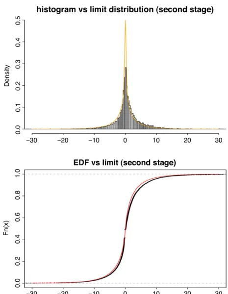
This section analyzes the empirical distribution of the second stage change point estimator

ˇ

τ and compares it with its theoretical counterpart. The empirical distribution is considered for a sample size of n = 5000 observations under the setup of the first experiment. Due to

mixed-normal type limit, in order to obtain the limiting distribution, a preliminary studentization of the sequencenθ_n2(tˇ_n −t∗)is required. Therefore, the limiting distribution of the following sequence

is studied

Zn =nθ_n2(tˇ_n −t∗)Γˆ(X_t∗, θ₀),

with _Γˆ₍_X

t∗, θ₀) = (log(1 + X2

t∗))2. Then Zn converges in distribution to W(v)− 1₂|v| with

density f(x)= 3 2e |x|  1−Φ 3 2  |x|  − 1 2  1−Φ 1 2  |x| 

and distribution function

F(x)= 

g(x), x > 0,

(25)

Fig. 1. Histogram versus theoretical density function (up) and empirical distribution function versus theoretical distribution function (bottom) for the second stage change point estimator. Results of 10, 000 Monte Carlo replications and sample sizen=5000 for the first model.

HereΦ(x)the distribution function of the Gaussian random variable, and

g(x)= 1+  x 2πe −x₈ − 1 2(x +5)Φ  − √ x 2  + 3 2exΦ  −3 2 √ x 

(see e.g. [5]). Fig. 1 reports the graphical representation of the histogram and empirical distribution function of Z (over 10,000 Monte Carlo replications) against their theoretical counterparts. The empirical results are inline with the expected theoretical quantities.

Acknowledgments

The authors wish to thank an anonymous referee for careful reading of the manuscript and fruitful remarks that led to an improved version of the paper.

References

[1] J. Bai, Least squares estimation of a shift in linear processes, Journal of Times Series Analysis 15 (1994) 453–472. [2] J. Bai, Estimation of a change point in multiple regression models, The Review of Economics and Statistics 79