Andean Competitiveness Project. Working Papers

(1)

W orking Papers

Natural Resource Dependence, Volatility and Economic Performance

in Venezuela: the Role of a Stabilization Fund

Lino Clemente, Robert Faris, and Alejandro Puente

February 2002

* Venezuela Competitiva

** Center for International Development, Harvard University

*** Instituto de Urbanismo, Universidad Central de Venezuela

(2)

LIST OF TABLES

Table 2.1. Importance of the Oil Sector in Venezuela……….15

Table 3.1. Analysis of relevant variables………...22

Table 3.2. Integration test for relevant variables………...23

Table 4.1. Aggregate Volatility Indicators Results – Positive Price Shock………34

Table 4.2. Impact of Positive Price Shock on Producer Prices in Domestic Currency………...36

Table 4.3. Aggregate Volatility Indicator Results – Negative Price Shock……….37

Table 4.4. Impact of Negative Price Shock on Producer Prices in Domestic Currency………..38

Table A.1.1. Current oil-related fiscal structure in Venezuela………46

Table A.2.1. Estimated contributions to the FIEM (US$ Millions)………...57

Table A.3.1. Results of a Dicky-Fuller Test with Four Lags………..63

Table A.3.2. Results of a Dickey-Fuller Test on WTI Crude Prices………...64

Table A.3.3. Results of a Dickey-Fuller Test on WTI prices since 1870……….65

Table A.3.4. Results of the Autoregressive Model………66

Table A.3.5. Results of the Kalman Filter Model………..68

Table A.3.6. Venezuelan crude price index projections (1996 US$/barrel)………...…69

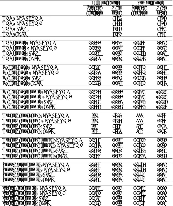
Table A.4.1. Aggregate Volatility Indicator Results – Negative Price Shock……….71

Table A.4.2. Aggregate Volatility Indicator Results – Positive Price Shock………...72

(5)

Natural Resource Dependence, Volatility and Economic

Performance in Venezuela: the Role of a Stabilization Fund

LINO CLEMENTE, ROBERT FARIS, and ALEJANDRO PUENTE

Acknowledgements: The authors are thankful for helpful comments, suggestions and information from Alejandro Grisanti, Ricardo Hausmann, Roberto Rigobón, Osmel Manzano, and Joaquin Vial, as well as the participants to the May 2001 Workshop on External Shocks at Harvard University sponsored by the Andean Competitiveness Project.

(6)

INTRODUCTION

Latin America has been hurt by a series of economic shocks instigated by such events as the precipitous changes in oil prices of the past three decades, the periodic contraction in international credit and the currency crises of the past few years. Venezuela is particularly susceptible to volatility with severe implications on its economic performance. The IDB (1995) estimates that annual growth in Venezuela has been more than 3% lower than it would have been otherwise had there been no volatility.

When an economy undergoes a shock, the impacts can permeate every corner of the economy. The level of economic activity (GDP) can change, and with it the level of employment. The real exchange rate, one of the key determinants of a country’s international competitiveness, can go through large movements, as can the relative performance of different domestic sectors, both tradeable and non-tradeable. Government budgets can be hit hard. Interest rates can undergo rapid fluctuations, affecting the financial health of corporations and the banks that depend on them, creating tensions in the entire national financial system. Finally, changing expectations of international markets regarding the solvency of the country can lead to self-fulfilling crises, destabilizing the macroeconomic climate.

In an economy susceptible to unanticipated shocks, economic agents must confront not only those shocks that have occurred but also those that might occur. This mix of uncertainty and instability has been termed volatility. Volatility affects countries’ real economic performance as well as their perceived level of risk. 1

Some countries are more susceptible to shocks than others. As established by the IDB (1995), the Latin America/Caribbean region has experienced more volatility than any other in the world with the exception of Africa and the Middle East. In volatile regions (or countries), GDP, employment, consumption, inflation, and investment tend to vary more erratically than in more stable areas. There is also evidence that productivity, poverty, income distribution, educational progress and strength of the financial system are negatively affected by greater macroeconomic volatility. The economic cost of volatility reveals that reducing and/or managing volatility offers potential benefits.

1_{Volatility and uncertainty are, in principle, two distinct concepts. Volatility refers to the tendency for a variable to fluctuate, while uncertainty exists} only when those fluctuations are unpredictable. Nevertheless, in practice those quantities which are volatile tend also to be unpredictable, diminshing the relevance of this formal distinction. The most common unit of measurement to determine the degree of instability present in a variable is standard deviation, which represents the typical deviation of a variable from its mean value. See IDB (1995).

(7)

External shocks that affect the terms of trade and capital flows are an important determinant of a region’s macroeconomic volatility and economic policy volatility. Moreover, important interactions between those shocks and economic policy must be considered in the design of policies and institutions intended to deal with unexpected shocks.

The principal cause of terms of trade volatility in Latin America—particularly in Venezuela—is the concentration of its exports in primary products whose selling prices are highly volatile. This lends great importance to policies intended to diversify exports and develop other strategies for reducing the risks associated with primary product exports.

Venezuela is one of the most volatile countries in the world, due to its (albeit decreasing) dependence on petroleum products subject to international price and production volume fluctuations (IDB 1995). It was nevertheless not until November 5, 1998, in the middle of a negative petroleum shock, that a lame-duck administration was able to push through the Macroeconomic Stabilization Investment Fund (in Spanish, Fondo de Inversión para la Estabilización Macroeconómica, or FIEM). The law establishing the Fund states it purpose as “preventing fluctuations in petroleum-related income from affecting the country’s necessary fiscal, exchange rate, and monetary balance.”2_{Curiously, the rules} governing the Fund have been changed twice since the original passage of the law, most recently on October 4, 2001 (see Vera and Zambrano 2001).

To date, research on stabilization funds in Venezuela has consisted of 1) studies preceding the Fund’s creation and focusing on its feasibility and optimal rule structure (Hausmann 1990, Hausmann & Powell 1990, Hausmann, Powell and Rigobón 1992); 2) statistical analyses of oil price series and their implications for stabilization funds’ operations (Rigobón 1999 and Grisanti 2000); 3) estimations of the contribution of a stabilization fund relative to existing laws and international comparisons of rule structures for stabilization funds (Fasano 2000); and 4) the implications of continuing reforms to the FIEM law (Vera & Zambrano 2001).

The goal of the present work is design a multisectoral dynamic computable general equilibrium (CGE) model based on a Social Accounting Matrix (SAM) in order to evaluate the impact of stabilization mechanisms on Venezuela’s macroeconomic balance. The model will take into account the Fund’s medium-term investment plans, a variety of global and sectoral variables such as the exchange rate and fiscal policy, and the Fund’s effects on factor allocation and income distribution

(8)

within the country. The analysis seeks to contribute to the volatility policy debate by evaluating institutional alternatives for the Fund’s management as well as its macroeconomic, sectoral, and institutional effects.3

Recent complementary studies using a similar empirical framework include Sachs and Warner (1995) and, for the case of Venezuela, Rodríguez and Sachs (1999). These works, however, focus mainly on the implications of natural resource abundance for medium-term economic growth.

The present work is organized into five sections. The first section presents the relationship between risk, volatility, policies, transmission channels and shocks—focusing on the case of Venezuela. The second section addresses the importance of the petroleum sector in the national economy. The third section analyzes stabilization funds as a mechanism for attenuating the effects of oil price oscillations—again highlighting the Venezuelan experience. The fourth section presents the analytical framework and simulation results. The fifth section concludes and discusses possible extensions of the work.

2_{The text of the law reads: “…procurar que las fluctuaciones del ingreso petrolero no afecten el necesario equilibrio fiscal, cambiario y monetario del país”.} 3_{Clemente and Puente (2000) review existing studies carried out in Venezuela that employ general equilibrium models.}

(9)

1. RISK, VOLATILITY, POLICIES, AND TRANSMISSION CHANNELS

The countries of Latin America have been characterized in recent years by significant volatility among a broad range of real and financial variables that are proxies for macroeconomic stability that is critical for economic development. This has placed them at a disadvantage relative to other regions of the world, where changes in the those variables are less abrupt and more predictable (IDB 1995, Caballero 2001). This remains true inspite of reform programs instituted during this period.

Risks confronting economic agents come from two sources. First, they can reflect aggregate volatility which, in turn, results from world goods and financial markets, volatile fiscal or monetary policies, or other exogenous factors. The speed and extent of these shocks’ transmission to agents’ incomes and internal economic policies depend on market structure as well as the policies and institutions that govern the country. Second, these risks can spring from microeconomic or sectoral volatility, which have no necessary relation to aggregate disturbances.

It must be kept in mind that external factors are not the only cause of volatility in developing countries, since macroeconomic policies must bear part of the responsibility. Policy volatility—though partly resulting from errors of the governments that design it—is largely the product of large external shocks to financial and insurance markets as well as weak domestic agencies whose hands are frequently tied by their limited mandates.

Recent experience suggests that monetary policy volatility has been consistently high in Latin American countries. Over the last two decades, the region has been noted for recurring episodes of hyperinflation produced by the monetization of unsustainable fiscal deficits. Fiscal volatility is closely related to monetary instability, as inflationary responses to fiscal disequilibria have been among the principal causes of volatility in monetary aggregates in the developing world—including Latin America prior to the 90s. The two variables show a clear, positive correlation (World Bank 2000).

The volatility of macroeconomic policy nevertheless reflects the effects of external shocks on the domestic economy. This is particularly true in those countries where the public sector depends on income generated by primary products, such as in Chile, Ecuador, and Venezuela. In these countries terms of trade shocks have an immediate impact on the external sector and government income, and are clearly reflected in fiscal aggregates. Fluctuations in the terms of trade are apparently an important

(10)

The extent of large shocks’ impact is determined by the market structure, institutions and policies that play a key role in either absorbing or amplifying those shocks. Among these mechanisms, domestic and global financial markets may be the most important—especially since the mid-90s. But in most Latin American countries, weak links between global and domestic financial markets, often shallow and poorly functioning, greatly amplify shocks rather than helping accommodate them. This double weakness in financial markets is at the heart of recent Latin American macroeconomic volatility (Caballero 2001). Financial market imperfections in Latin America and the Caribbean strictly limit fiscal smoothing and the diversification of risk (Hausmann 2001 and World Bank 2000).

This propagation effect is especially evident in the banking system. As adverse shocks cause difficulties for domestic firms, the banking system’s credit portfolio can deteriorate, in turn reducing the ability and willingness of the system to take on new risks and allocate resources efficiently. Certain borrowers can become barred from the credit market, only exacerbating the situation. When the financial position of the banking system is compromised, this sequence of events can bring banks to the brink of financial collapse, dragging even financially healthy borrowers down with them.

Weak capital markets also amplify the effects of shocks. Just as weak banking systems can lead to credit rationing, capital market failures can result in what might be termed “equity rationing”—the inability of firms to raise equity capital without incurring prohibitive costs.

The connection between underdeveloped financial markets and economic instability can be clearly seen on the international stage. In cross-country data, a larger domestic financial sector is correlated with lower levels of economic volatility—although this relationship weakens when financial sectors become extremely large. A rapid expansion of financial systems, particularly when poorly regulated and inadequately supervised, can also contribute to economic volatility (World Bank, 2000).

In addition to the financial system, there are other institutional and political factors that play a key role in either magnifying or containing the economic impact of shocks to the domestic economy. They include:

! Fiscal policy—frequently in the form of “automatic stabilizers”—consists of compensating for negative shocks with a corresponding expansion of aggregate demand, or reduction in the case of positive shocks. In Latin America and most of the developing world, however, fiscal policy is markedly pro-cyclical. This serves to accentuate expansion in booms as well

(11)

as aggravate the contraction of recessions. Instead of compensating for shocks, then, fiscal policy can add to their attendant economic risk. To a certain degree this reflects the influence of financing constraints, as in recessions governments face drastic reductions in their access to foreign finance or large increases in its cost (Talvi and Végh 2000).

! Exchange rate and monetary policy can enable the domestic economy to weather the effects of external shocks. In this case, the objective must be to achieve a balance between credibility and flexibility over time. There are no easy recipes for successful monetary and exchange rate policy. Key elements of a policy that is viable on the medium term include simple and transparent rules and standards that are well adapted to the country’s economic, political and institutional reality.

As in the case of other aggregate shocks, risk diversification is the best response to terms of trade volatility. This diversification can be achieved by selling, on international markets, the rights to a portion of future commodity revenues. In this way, domestic agents need not suffer the full impact of their volatility and can instead hold other assets instead (Engel & Meller 1992). The use of international futures markets—through the sale of future copper or oil production at prices fixed in advance, for example—is another way to diversify terms of trade risk. But in spite of their growth in recent years, futures markets remain limited. Futures prices often undergo great fluctuations, and the markets’ operations remain focused on short-term instruments.

In view of insurance market limitations, various Latin American and Caribbean countries have resorted to self-insurance, in the form of commodity stabilization funds in order to manage terms of trade risk. These funds are designed to accumulate funds in periods of high commodity prices, to be drawn down when prices fall below a predetermined “reference” level. In contrast to true insurance, stabilization funds do not involve any true diversification of risk; rather, they merely transfer funds from good states of the world to bad. They also involve significant opportunity costs, as accumulated funds must be held in short term instruments and thereby forego the more attractive returns of less liquid investments. Engel and Meller (1992) review the experience of Latin American stabilization funds while Hausmann, Powell and Rigobón (1992) conduct a preliminary evaluation of Venezuela’s FIEM.

(12)

of commodity price fluctuations by reducing the concentration of imports in a limited number of primary products.

In order to reduce the impact of external volatility on the domestic economy and encourage sustainable development strategies, an essential first step is to identify the channels through which shocks are transmitted. Recent studies suggest that fiscal expenditures can be the most important transmission channel, highlighting the importance of fiscal institutions and the application of fiscal rules (see Alesina, Hausmann, Hommes and Stein 1999 for a review of this issue focusing on Latin America and the Caribbean).

It is crucial that fiscal policy maintain its dual objectives of solvency and liquidity over time. Stabilization funds can help achieve this through numerical and procedural rules to guarantee their transparency and long-term viability. Other factors critical to success are effective management of international reserves, international debt policy, and political will (Engel & Valdes 2001 and Hausmann 2001).

In Venezuela, oil shocks are transmitted to the domestic economy via two principal paths— through fiscal expenditures, and through the terms of trade. Both impacts eventually affect expectations of the country’s solvency and, without doubt, the medium-term performance of the real economy. If the shock is positive—that is, related to a rise in oil prices—there can be a sudden increase in the budget surplus and current account, followed a few months later by a rise in domestic public spending, especially when the next budget is negotiated. The result is pro-cyclical fiscal behavior. The new expenditures put upward pressure on aggregate demand, stimulating an increase in imports as well as an increase in the prices of tradeables due to short-term supply rigidities. This increase in non-tradeables prices can generate inflationary pressure, producing an appreciation of the real exchange rate, since during an oil boom the nominal exchange rate tends to remain stable.

This real appreciation in turn produces a twofold effect. First, it further stimulates imports, which have become cheaper relative to their domestic counterparts. Second, the fiscal balance can deteriorate.4_{Both effects combined can generate, over time, a deterioration of the current account as} oil prices begin to fall below the local maximum achieved during the shock. Oil prices, public

4_{The favorable fiscal effect of a devaluation depends on how long inflation takes to match the pace of depreciation or devaluation that has occurred.} The greater the degree to which the depreciation or devaluation of the currency is maintained in real terms, the more lasting will be the positive fiscal effect. On the other hand, the more rapidly domestic inflation adjusts to the rate of devaluation or depreciation, the more fleeting will be the fiscal effect (Clemente & Puente 2001).

(13)

spending, and the real exchange rate are clearly the variables revealing the effects of adjustment in both macroeconomic aggregates.

When the shock is negative—resulting from a fall in oil prices—ordinary fiscal revenues are significantly affected and measures to reduce public spending become necessary. Nevertheless, there are restrictions that ensure a temporal disconnect between the moment the shock occurs and the opportunity for budget institutions to react by raising income and/or lowering expenditures, thereby adapting internal absorption to the new equilibrium. This lack of policy coordination and/or institutional adaptation shows up in a greater fiscal deficit or lower surplus in the current account. Adjustment measures necessary to correct the disequilibrium can bring the economy into recession.

The other mechanism through which oil shocks are transmitted to the domestic economy is the terms of trade. Their effect can be seen not only in the exchange rate, where it can induce the expectation of depreciation, but also in slippage in the country’s indicators of solvency and the performance of tradeable goods sectors.

The volatility of oil income together with a lack of adequate institutional arrangements have resulted in pro-cyclical public expenditures. These have also subjected the economy to relatively short cycles, in which boom periods give way rapidly to crisis and recession, to be replaced shortly thereafter by recovery and a repetition of the cycle. This pattern obviously reflects not only the difficulties faced by monetary policy as well as the inability of fiscal policy alone to play a stabilizing role.5

5_{Blejer and Cheasty (1990) and Morgan (1979) show that in the case of publicly-owned primary product exporting countries, if the monetary impact of} this income is not sterilized, its use to finance public spending will inevitably lead to expansionary effects on the money supply. This is particularly true

(14)

Figure 1.1. Terms of Trade

(Export Price Index / Import Price Index)

0 0.2 0.4 0.6 0.8 1.0 1.2 1.4 19 50 19 52 19 54 19 56 19 58 19 60 19 62 19 64 19 66 19 68 ₁ 97 0 19 72 19 74 19 76 19 78 19 80 19 82 19 84 19 86 19 88 19 90 19 92 19 94 19 96 19 98 20 00 0 19 50 19 52 19 54 19 56 19 58 19 60 19 62 19 64 19 66 19 68 ₁ 97 0 19 72 19 74 19 76 19 78 19 80 19 82 19 84 19 86 19 88 19 90 19 92 19 94 19 96 19 98 20 00

Source: BCV, MEM, and authors’ calculations.

The interaction between fiscal policy, exchange rates, and inflation has contributed to the instability of economic growth in Venezuela, since exchange rate adjustment to correct fiscal disequilibria and the associated contractionary effect of devaluation has had negative repercussions on growth.6

(15)

2. VENEZUELA: AN OIL ECONOMY

Until the 1920s Venezuela was a rural, agricultural country whose primary exports were coffee and cocoa. Since that time, the discovery of large domestic oil deposits as well as high demand from the United States and Europe have contributed to extensive development of the petroleum industry. In Venezuela, oil was seen as a fiscal resource for the modernization of an agricultural, rural country when the Great Depression of the 1930s provoked a collapse of coffee and cocoa prices. Subsequent development of global oil markets allowed petroleum products to become and remain Venezuela’s primary export. A national discussion on the role of the oil industry in Venezuela’s destiny began in 1936 and intense debate continues to the present day (Clemente and Puente 2001). The relative importance of the petroleum industry in real economic activity (GDP) began in the 1920s and came to represent 31% of the economy by the 1960s. Its importance fell to just 20% by the 1980s, but by the 1990s recovered to 25% of GDP.

The high volatility of oil income is principally reflected in the balance of payments and the fiscal balance, due respectively to the relative importance of oil in exports and in fiscal revenue. This importance has, however, diminished since the 1970s. This can be seen in the fact that the positive oil shock of 2000 affected these variables to less than 40% of the degree to which they were affected by the 1974 shock.

Table 2.1.

Importance of the Oil Sector in Venezuela

Indicators (%) 1970-79 1980-89 1990-99

Oil revenues/GDP 15.1 13.2 11.4

Oil revenues/Total government revenue 70.1 60.7 59.0

Oil exports/Total exports 87.4 82.2 71.1

Oil exports/GDP 23.0 21.2 20.5

Real oil GDP/Real total GDP 31.3 20.0 24.5

(16)

Figure 2.1.

Current Account and Fiscal Balance (as % of GDP)

The non-oil sector in Venezuela is highly dependent on oil income and, consequently, on fiscal policy. This dependency severely restricts the freedom of monetary policy by making it essentially endogenous in respect to public spending.

-20 -15 -10 -5 0 5 10 15 20 19 75 19 76 19 77 19 78 19 79 19 80 19 81 19 82 19 83 19 84 19 85 19 86 19 87 19 88 19 89 19 90 19 91 19 92 19 93 19 94 19 95 19 96 19 97 19 98 19 99 20 00 % -20 -15 -10 -5 0 5 10 15 20 19 75 19 76 19 77 19 78 19 79 19 80 19 81 19 82 19 83 19 84 19 85 19 86 19 87 19 88 19 89 19 90 19 91 19 92 19 93 19 94 19 95 19 96 19 97 19 98 19 99 20 00

Current Account / GDP (%) Fiscal surplus (deficit) / GDP (%)

% Oil

Embargo _RevolutionIranian

Iran-Iraq War Gulf War Iraq-USA Conflict Repercussions of Asia and OPEC accords

(17)

Figure 2.2

Venezuelan oil exports per capita

This means that, in general, monetary policy must be counter-cyclical to public expenditure, complicating regulation of the money supply during fiscal expansions. At these times, the Central Bank must compensate for the expansion by absorbing excess resources from the economy.

In an economy like Venezuela’s, with a high degree of dependence on oil income7_{and a tight} link between oil income and fiscal expenditures, oil income volatility will be reflected in monetary aggregates unless the Central Bank or a stabilization fund adequately sterilizes income that is incompatible with inflationary or long-term debt objectives.8

1.500

2.500

3.500

4.500

19 70 19 72 19 74 19 76 19 78 19 80 19 82 19 84 19 86 19 88 19 90 19 92 19 94 19 96 19 98 20 00

500 1,500

2,500

3,500

4,500

19 70 19 72 19 74 19 76 19 78 19 80 19 82 19 84 19 86 19 88 19 90 19 92 19 94 19 96 19 98 20 00 Millions of US$

(18)

3. NONRENEWABLE RESOURCE FUNDS AND THE

MACROECONOMIC STABILIZATION INVESTMENT FUND (FIEM)

IN VENEZUELA

Stabilization funds are designed to reduce volatility by transferring resources from good years to bad. This is generally accomplished by accumulating money in a fund when economic circumstances are favorable, such that these funds can be draw upon in bad times. The economic and practical logic of smoothing out fluctuations caused by unexpected events is both compelling and fairly obvious.

The advantages on the real economy are several. Reducing fluctuations in the government budget will improve the continuity of critical public programs and increase the scope for carefully planning and implementing public projects. For the poorest segments of society, smoothing aggregate consumption will reduce temporary but potentially catastrophic declines in income. Reducing volatility in consumption will also reduce risk and costly risk aversion strategies, opening the way for potentially more profitable production possibilities. A steady course of aggregate investment will facilitate project selection and implementation and enhance maintenance of capital stocks, increasing the return on current and prior investments.

In addition to reducing the debilitating effects of frequent economic expansions and contractions, reducing changes in relative prices such as those mediated through the real exchange rate will provide solid benefits for producers. Finally, reducing volatility will reduce the problems associated with financial and monetary swings. The government will have an easier time maintaining macroeconomic balances, keeping inflation in check while promoting growth. Alleviating financial fluctuations will improve the depth of the financial system, providing benefits for the productive and financial sectors.

There are a variety of mechanisms and objectives for commodity and natural resource funds. Heritage funds are designed to increase overall national saving, aiming to smooth consumption over time by transferring wealth to future generations. The objective of heritage funds centers on the question of optimal savings. This is an economic issue that differs from the question of allocating financial assets, deciding whether to assign a fiscal surplus to financial assets or to invest these funds into public works or other capital creation efforts (Davis et al 2001).

(19)

Venezuela displays the key characteristics that would make it an obvious place to consider a heritage fund – a high portion of national income coming from a non-renewable resource – except that the high incidence of poverty makes such a strategy economically questionable and politically difficult. In this paper, we consider only the implementation of a stabilization fund that targets financial objectives rather than the question of optimal savings (see Grisanti 2000). In considering the financial issues, we attempt to smooth the inter-temporal allocation of national savings to reduce volatility. This strategy has the additional benefit of helping to ward off short-term financial crises, which are seen by some to be the most serious cost of volatility (Caballero 2000).

In theory, the stabilization fund could be operated by borrowing when prices are low and paying back the loan when prices are high. However, this is unrealistic in practical terms for two reasons. First, international financing is generally not available in adequate amounts in bad times. International financial markets will usually allow the country to borrow in good times (as they did in the 1960s in Bolivia), but when the country is hit by an adverse shock it may well lose its creditworthiness and face a decline in its borrowing capacity just when it needs it most. Second, the temptation of high revenues often leads to increased borrowing during good times rather than the opposite as suggested above. Because of these factors, stabilization funds must generally start by accumulating funds in order to be brought into operation. This reduction in current expenditures entails a cost of instituting the stabilization fund in the form of reduced consumption and lost investment and thus lower capital stocks and decreased production. The benefit of a stabilization fund thus has to be judged against this cost.

The accumulation of funds is one of the primary objectives of heritage funds. For a stabilization fund under consideration in here, we should prefer to minimize the amount of resources in the fund for a given level of volatility reduction. This is one the fundamental tradeoffs in designing a stabilization fund, limiting the amount of resources tied up in the fund while ensuring that adequate funds are available to achieve the desired stabilization objectives.

This of course assumes that returns to capital will be higher on equity participation in domestic investment projects than in holding foreign assets. Furthermore, we generally assume that returns to investment, or the fraction of the resources channeled into investment, are the same over different time periods. If for some reason waiting to carry out investments will increase the return on investment, then holding the resources in the fund abroad will provide benefits above those that stem from

(20)

Venezuela created the Macroeconomic Stabilization Investment Fund (FIEM) in 1998 to address the problem of volatility as the result of fluctuations in the price of oil. As we detail in

Appendix 2, FIEM has undergone a number of changes since its inception. Based on the last revisions, the government will make contributions as a fixed proportion of fiscal revenues from petroleum into FIEM from the years 2003 through 2007. These contributions will start at 6% and increase by one percentage point each year until 2007. Starting in 2008, the fund will operate according to its originally developed rules. Revenue benchmarks will be calculated for government fiscal revenues and PDVSA export earnings based upon five year moving averages. Deposits and withdrawals into the fund will subsequently be made by comparing current revenues to these benchmark figures.

The FIEM deals with the issue of accumulating excessive resources in the fund by creating an upper limit on contributions into the fund. If fund resources are greater than 80% of a 5-year average of petroleum export revenues, then the surplus is funneled back into PDVSA accounts, national investment funds and paying down the debt. Further details about the FIEM can be found in Appendix 2. In a later section, we will assess the performance of the FIEM as it is currently planned in reducing macroeconomic volatility, versus two alternative designs.

The formulation of a stabilization fund does not by itself ensure that these macroeconomic objectives will be reached. Government funds are fungible, and it is well recognized that such a stabilization fund can be easily rendered ineffective if the government carries out an otherwise pro-cyclical fiscal policy, borrowing to increase expenditures during good years. This is in fact what appears to happened in Venezuela for the initial years of the stabilization fund. Public debt increased during this period, resulting in greater indebtedness rather than accumulated wealth. A stabilization fund will only be effective if it is accompanied by either borrowing constraints or by a program of fiscal

discipline that eschews the temptation of pro-cyclical spending.

In fact, conservative fiscal policy by itself has the potential to achieve the same stabilization objectives. Much of the success and attractiveness of a stabilization fund is in its ability to foster fiscal discipline that would not otherwise occur. The political economy arguments for stabilization funds are as follows: 1) The existence of the Fund could reduce pressure on the government to raise expenditures in the event of rising revenues; 2) the implementation of the Stabilization Fund could be an opportunity to enact complementary fiscal rules that reduces the scope for borrowing and spending by the

government; 3) it might be politically difficult to issue public debt in order to make planned payments to the Stabilization Fund. Normally the government would borrow when oil prices are high and in that

(21)

way cause pro-cyclical spending. The very existence of a stabilization fund may make it more difficult for governments to issue new debt (Davis et al 2001).

3.1 The future of oil prices: Considerations for designing a stabilization fund

The stochastic behavior of petroleum prices and income is a critical element to consider in designing a stabilization fund for Venezuela. Knowledge of this underlying process is important not only to establishing the rules under which the fund operates but also the metrics by which its performance is to be measured. A principle question regarding the behavior of oil prices is whether they are stationary. If the price of oil is stationary, then following a shock the price will revert to the mean value, or trend: fluctuations in the price of oil in this context would be temporary. Within fiscal constraints, stabilization policy could then attempt to correct for all of the stochastic volatility. If oil prices are nonstationary, then oil shocks have a permanent effect on oil prices, and the question becomes how to adjust to the new level. In this case, however, Hausmann, Powell and Rigobón (1992) posit that a stabilization fund might still minimize the necessary adjustment costs.

As is extensively discussed in the related literature, a series of theoretical and practical difficulties complicate the exact characterization of the stochastic process. One interesting study is that of Eduardo Engel and Rodrigo Valdés, who evaluate 12 different models or variants of predictive models (out of sample) of oil prices.9_{The authors reach the conclusion that the best predictors are a} simple random walk and an ARIMA model. They nevertheless point out that despite the difficult in rejecting the null hypothesis of nonstationarity of the series, theory suggests that this result may arise from sampling problems. Intuitively, this is because oil prices cannot long remain below the marginal cost of production, and conversely, high oil prices will stimulate production of oil as well as its substitutes—driving down the price. Another explanation suggested by Engel and Valdés relies on possible nonlinearities in the adjustment process. That is, the price may behave as a random walk only within a certain range, outside of which stabilization forces dominate. Another point raised by Engel and Valdés is the possibility of structural changes in the economy, since their conclusions vary depending on the number of years included in the analysis.

Pindyck (1999) proposes that such stationarity tests, when applied to small samples, may have very low power. Rigobón (1999) applies the methodology proposed by Pindyck, reaching similar conclusions. Table 3.1, below, reproduces some related work by Grisanti (2000) regarding the

(22)

following oil prices, production volume, real exports, and per-capita real exports. The variables shown are in logarithms and the first differences of their values, maxima, minima, and standard deviations may therefore be interpreted as percent changes.

Although precise conclusions to be drawn from these data depend on the time period considered, general results include: a large year-to-year variation in the series, non-normality of distribution (shown in the positive skewness of prices, negative skewness of volumes, and high kurtosis), and significant first- and second-order autocorrelation of the variables.

Table 3.1.

Analysis of relevant variables (Logarithms and first differences)

Real price of WTI (West Texas Intermediate) oil, 1879-1999 Real price of Venezuelan oil, 1820-1999 Export volume

1925-1999 Real oil exports 1925-1999 Real oil exports per capita

1925-1999

Level 1st_Diff. _Level ₁st_Diff. _Level ₁st_Diff. _Level ₁st_Diff. _Level ₁st_Diff.

Sample size 130 129 80 79 75 75 75 75 75 75 Average 2.64 0.00 2.43 0.00 0.57 0.03 8.96 0.04 6.70 0.01 Minimum 1.93 -0.66 1.83 -0.67 -0.95 -1.46 6.94 -0.56 5.58 -0.59 Maximum 3.70 0.71 3.63 0.87 1.24 0.35 10.10 0.73 7.61 0.70 Std. deviation 0.33 0.21 0.48 0.19 0.59 0.13 0.82 0.22 0.44 0.22 Skewness 0.74 -0.10 0.95 0.54 -1.10 -0.60 -0.90 -0.20 -0.50 -0.20 Kurtosis 4.12 4.42 2.76 7.97 3.40 6.08 3.05 4.70 2.60 4.58 Jarque-Bera 18.60 11.10 12.20 85.10 13.00 29.40 9.30 7.90 2.60 6.85 Probability 0.00 0.00 0.00 0.00 0.00 0.00 0.01 0.02 0.27 0.04 1 0.91 0.02 0.92 -0.10 0.93 0.00 0.92 -0.10 0.85 -0.10 2 0.82 -0.20 0.86 0.02 0.86 0.21 0.86 -0.10 0.73 -0.10

Note: ρ1 and ρ2 indicate, respectively, first- and second-order autocorrelation coefficients. Source: Grisanti (2000)

The high volatility of these variables can be seen in the figures for standard deviation and kurtosis. The skewness of the production volume distribution more than makes up for that seen in prices, producing a negative skewness in real export income and indicating a larger number of years with prices below the mean than above it. Finally, the high degree of first- and second-order

9_{“Optimal Fiscal Strategy for Oil Exporting Countries,” IMF Working Paper, June 2000.}

(23)

autocorrelation reflect the great inertia in oil price, volume, and income cycles as well as the slow rate of mean reversion.

The stationarity analysis carried out by Grisanti is reproduced in Table 3.2. In this analysis, the variables were equally defined in logarithms of price levels (for different periods in the case of WTI), volumes, real exports and real exports per capita.

Table 3.2.

Integration test for relevant variables

DF ADF (2) ADF(4) ADF(8) Sample C CT C CT C CT C CT

Real crude price (WTI)

Log level 1% 1% 1% 1% NO 10% 5% 1% 1870/

Log difference 1% 1% 1% 1% 1% 1% 1% 1% 1999

Real crude price (WTI)

Log level 10% NO NO NO NO NO NO NO 1920/

Log difference 1% 1% 1% 1% 1% 1% 5% 10% 1999

Real crude price (VEN)

Log level NO NO NO NO NO NO NO NO 1920/

Log difference 1% 1% 1% 1% 1% 5% 10% NO 1999

Export Volume

Log level 1% 1% 1% 1% 5% 5% 5% NO 1920/

Log difference 1% 1% 1% 1% 1% 1% 5% 5% 1999

Real crude exports

Log level 1% 1% 1% 1% NO NO NO NO 1920/

Log difference 1% 1% 1% 1% 1% 1% 1% 1% 1999

Per capita real crude exports

Log level 1% 1% 1% 1% 5% NO NO NO 1920/

Log difference 1% 1% 1% 1% 1% 1% 1% 1% 1999

Notes: Critical values of DF= Dickey-Fuller and ADF(r)= augmented Dickey-Fuller with r lags. ‘NO’ indicates that the test was rejected at the 10% significance level. ‘C’ indicates that only the constant is included in the test, whereas ‘CT’ indicates that both the constant and a trend term are included.

Source: Grisanti (2000).

In general, the results indicate that the variables are stationary in levels, though the behavior of prices show mixed results. It is interesting to note that studies of the Venezuelan price index fail to reject the hypothesis of a unit root in levels, as does the same test applied to WTI (West Texas Intermediate) for the same time period, but when this latter test is extended to a longer time series the

(24)

result reverses. This suggests that the nonstationarity result for Venezuelan prices may be an artifact of small sample size.

Using this empirical basis, we calculate different international oil price scenarios used for the general equilibrium model. These price projections., which are presented in Appendix 3, feature a long-term price trend to which prices revert after negative and positive shocks are imposed. In considering the design and performance of a stabilization fund, the disparity between stationary and nonstationary price trends is not as pronounced when considering a slow reversion to the mean value. Moreover, the rationale for operating a stabilization fund applies in either case: there appears to be sufficient empirical evidence to recommend a stabilization mechanism for the Venezuelan economy.

(25)

4.

THE MODEL: DESCRIPTION, SIMULATIONS, AND RESULTS

In this section we will first describe the Computable General Equilibrium (CGE) model that we use, and then we will use the model to analyze the performance of the stabilization fund.

4.1. Specifying the key equations of the CGE model

The model developed for this study is a standard 3-sector recursively dynamic model. The three sectors described in the model are the petroleum sector, oil tradeables sector and the

non-tradeables sector. This three sector approach is intended to capture the most important intersectoral impacts of changing oil prices and the volatility this brings in the simplest possible terms. The

foundation of the model is a social accounting matrix constructed by the authors based on 1996 data. Capital is divided into two classes, that used by the petroleum industry and that used by the rest of the economy. In the model, investment in the petroleum is determined exogenously, and is based on PDVSA projections. Employment in the petroleum sector is treated in the same manner.

Labor is divided into three classes, urban skilled, urban unskilled and rural. To reflect the medium-to-long term time horizon, we allow labor to migrate between the rural sector and the urban unskilled sector. There are four household categories defined according to the source of income.

In the petroleum sector, production is fixed exogenously according to industry forecasts. For the tradeable and non-tradeable sectors, output, prices and factor demands are all determined endogenously within the model. Production is portrayed with a multiple-stage nested function. Labor and capital are combined in a Cobb-Douglas relationship to produce value added. Value added and composite intermediate goods are then pooled in a constant elasticity of substitution (CES) function. Domestic intermediate inputs are used in fixed proportions to form the aggregate domestic intermediate factor. Imported intermediate goods are combined with domestically produced intermediates using a CES function. This formulation is constructed to reflect the flexibility in production choices for medium to long-term processes.

(26)

Figure 4.1. Production Functions for the CGE Model

Production

Value Added Composite Intermediate Good

Labor Capital

Imported Domestic

Intermediate Goods Intermediate Good

As one of the principal foci of this analysis is the study of the accumulation of capital in the face of price volatility, the treatment of capital is somewhat distinct from what is generally found in these models. Using a putty-clay depiction of capital, factors become more rigid in the production process once capital has been installed. Following Jacoby & Wing (1999), we assume that a given portion of capital is converted to a fixed coefficient production function after each investment period, in this case one year. This builds into this model a production context where managers cannot freely substitute intermediates, labor and capital in response to changes in wage rates and the cost of capital. This creates a context whereby prior investments made upon expected future relative prices can lock producers into sub-optimal production technologies.

The model is solved recursively over a thirty-year time horizon. The model is run for each time period, after which the stocks of accumulated factors are updated before the model is run again for the next period. The key aspect of defining the dynamic relationship in a macroeconomic model is the treatment of savings and investment behavior. In this model, aggregate investment is determined by national savings. First, savings is fixed as a fixed percentage of income for households and corporations according to their observed marginal propensity to save. Government savings is determined endogenously as the remainder after predetermined expenditures are subtracted from current revenues. In the absence of a solid empirical basis for estimating foreign savings levels, these are set exogenously

(27)

as a percentage of GDP using historic levels. Once the level of aggregate savings is determined, the allocation of investment is determined by relative profitability based upon current prices. This is an alternative formulation to fully dynamic models where consumers and producers make savings and investment decisions based upon perfect price information for all future periods, recognizing that decision-makers are imperfect predictors of the future.

Factor demands are determined by profit maximizing behavior. Two types of rigidities are built into the model to better mirror reality. Firstly, investment decisions are made according to prices that prevail at the time of the decision. This acts as a proxy for expected prices. This investment is committed to the sector, even though prices will have changed when the investment is brought into production in the next time period. This means that investment decisions, and hence capital allocation decisions, are made with imperfect information regarding future prices, allowing for the sub-optimal allocation of capital. The second rigidity arises from the putty-clay formulation of capital mentioned earlier. The combination of capital, labor and intermediates is made at the time of the investment decision. In future periods, a portion of the production process takes place with this less-than-perfect mixture of factors and inputs. The magnitude of both of these impacts varies with the size of relative price changes across different time periods.

The relationship between imports and domestically produced commodities, as well as the relationship between exports and domestically consumed commodities, are treated in the standard way for CGE models, using an Armington function for imports and a constant elasticity of transformation (CET) function for exports. This formulation entails the imperfect substitution between these different commodities which allows for two-way trade as in observed trade relations.

This permits the elasticity of substitution between imports and domestically produced goods for these different sectors to vary, and hence for scenarios to look at different taxation schemes and world price trends by import type.

Labor markets operate in the manner used by De Santis (2000). Using the empirical observations of Blanchflower & Osward (1994) and others, a relationship between real wage rates and unemployment is specified, where higher wages coincide with lower unemployment. The empirical basis of the ‘wage curve’ mimics a labor supply curve when specified in a simulation model. Thus the labor markets operate on the principles of supply and demand in the model, rather than the usual

(28)

choice between fixing wage rates or fixing labor supply curves. A full listing of the equations in the model are included in Appendix 5.

4.2 The costs of maintaining a stabilization fund

The economic cost of maintaining a stabilization fund is the result of setting aside a portion of petroleum revenues in a fund abroad rather than allowing these funds to be utilized within the economy. Reduced government expenditures and investments is the primary avenue, though PDVSA expenditures are expected to decline as well. We simulate these costs in the CGE model by comparing a scenario with the stabilization fund versus a scenario without the fund. Both of these initial scenarios are based upon baseline oil price projections.

The model predicts a growth rate for the Venezuelan economy of between 3 and 4 percent annually. Growth drops off after 2011 as we assume no further expansion of oil beyond that point. It is important to note that we do not suggest that this model will be a good predictor of future levels of economic growth. The model ignores the important influence of productivity gains on growth so that growth in production reflects factor accumulation only. While this is an important component of growth, it presents an incomplete picture. Secondly, this is a model of the real economy. Therefore, it does not incorporate the influence of financial and nominal factors on economic performance. Finally, we don’t presume to know what international prices will do over the next 25 years. This model is most useful in observing the difference in performance of the economy between different scenarios, rather than predicting accurately future levels of economic output.

The first question we approach is the cost imposed on the Venezuelan economy by the stabilization fund under the assumptions of the base scenario. Figure 4.2 shows that the cost in terms of growth and output is quite small. The drop in growth is the result of the Stabilization Fund drawing savings and investments away from the economy. Under this scenario, deposits are made into the Stabilization Fund from 2003 until 2007. After 2008, although revenues continue to grow, resources are withdrawn from the fund each year in order to maintain the maximum size of the fund below the ceiling. In relative terms, the fund reaches its maximum size in year 2008 as it approaches 20% of GDP. Wages are somewhat suppressed by the operation of the fund.

(29)

It is important to note that this model is well suited for accounting for the costs of the stabilization fund, yet does not account for many of the benefits. The benefits of reduced volatility, as summarized earlier, might be manifest in the economy through greater efficiency in capital creation, improved efficiency in factor utilization – bringing on higher returns to labor and capital and perhaps higher productivity growth – and higher overall rates of investment in the economy, both in physical and human capital, leading to higher rates of factor accumulation and productivity growth. While the theoretical and empirical cases for these processes are strong, the empirical work in this area has only taken place at a fairly aggregate level, leaving us without an adequate basis for simulating these benefits.10_{Nonetheless, if the benefits of reducing volatility are even a fraction of the estimates} presented earlier, it is easy to conclude that the benefits of reducing volatility will far exceed the costs.

We turn to the question of how well such a stabilization fund will perform in reducing volatility.

Figure 4.2. GDP growth with and without the Stabilization Fund

4.3 Performance of the stabilization fund in the presence of price shocks

We start by looking at the impact of positive price shock. Positive price shocks are generally considered a good phenomenon because of their expansionary tendencies. They do, however, bear potential complications. One of the ramifications of the relative price shifts is price volatility, 0.00 0.01 0.01 0.02 0.02 0.03 0.03 0.04 0.04 0.05 2001 2003 2005 2007 2009 2011 2013 2015 2017 2019 2021 2023 2025 G D P gr ow th

GDP growth - with fund GDP growth - base

(30)

particularly for the non-petroleum tradeable sector which will suffer from the expected appreciation of the exchange rate. If the shock is permanent, then the economy will adjust to a new equilibrium, with a difference composition of the economy. This is in itself not a problem. Rather it is frequent changes in prices, i.e. temporary shocks, that will cause the expansions and contractions of different sectors of the economy, reducing the profitability of all sectors. In a sense, the country is unable to establish its comparative advantage, as this is constantly changing. A commonly cited manifestation of this is where the tradeable sector is largely dismantled during a resource boom, and is then ill-prepared to take advantage of more favorable conditions during the inevitable downturn in international oil prices. A related set of issues arises out of the expectations that are generated during boom periods. For example, expectations of revenue and expenditure patterns by the government may lead to unsustainable levels of investment and unfinished public works programs.

A stabilization fund is primarily thought of as an instrument to cushion an economy from downturns in international oil markets. However, if the objective of the fund is to decrease volatility, then it has a role to play on both upturns and downturns. Smoothing the transition of the economy to changes in international oil prices applies equally to resulting economic expansions and contractions.

The trajectory of the price path for oil with a positive price shock, as estimated in the analysis summarized in Appendix 3, is presented in Figure 4.3. Using this price path, we run the simulations using four possible scenarios: 1) no stabilization fund – NO FUND; 2) the Venezuelan stabilization fund in its current configuration - FIEM; 3) and two alternative configurations for the stabilization fund – ALT FUND 1 and ALT FUND 2. We have created the alternative fund rules to test for their performance in correcting what we see to be problems with the FIEM.

(31)

Figure 4.3. Projected International Oil Price Paths with Positive and Negative Shocks

One apparent flaw in the FIEM is that it requires deposits from the years 2003 until 2007 regardless of the context, whether prices are low or high, falling or rising. This could create the situation where the stabilization fund exacerbates an economic downturn stemming from a drop in oil prices. This feature of the FIEM should be corrected with a contingent rule that only mandates deposits in years where oil revenues are better than average.11

The second aspect of the FIEM that may be improved is that a rigid upper limit has been placed on the size of the fund, and this limit has been set in respect to an average of recent export revenues. A priori, this seems like a poor choice for two related reasons. First, selecting past oil revenues as the relevant benchmark for the size of the fund introduces the possibility that the fund will be prevented from taking on further deposits in the event of significant price rise. This will occur with a rise in oil prices following a period of low oil revenues, which will have created a low upper limit on the size of the fund. If using an upper limit for the size of the stabilization fund, it is better to choose a benchmark based only on current revenues or, perhaps more appropriately, a benchmark proportionate to the size of the economy, for example, GDP itself. Second, a rigid upper limit to the fund will mean

11_{Although we do not report the results of simulations run with a negative price shock during the accumulation stage from years 2003-2007, the results are}

0.00 0.20 0.40 0.60 0.80 1.00 1.20 1.40 1.60 1.80 2.00 2002 2003 2004 2005 2006 2007 2008 20092010 2011 2012 2013 2014 2015 2016 2017 20182019 2020 2021 2022 2023 2024 2025 2026 In te rn a ti ona l oi l pr ic e i nde x

(32)

that deposits will be abruptly shut down and/or reversed to withdrawals without regard to the price path. This could, in fact, add volatility to the economy.

To correct for these aspects in the FIEM, we created ALT FUND 1, which has modified rules. First, it uses contingent rules in the initial 5 years of the fund identical to the long-term rules of the fund, comparing current revenues with an average of past revenues. Second, there is no ceiling on the size of the fund.

In place of a ceiling on the fund, the contingent rules of the fund are designed such that the size of deposits into the fund vary according to the size of the fund. For this feature, we use a simple formula to determine the percentage of the surplus in revenues above the benchmark that will be deposited (SFDPCT), where SFUND is the size of the fund in the domestic currency and GDP is real gross national product:

SFDPCT =1−α SFUND

GDP



  

β

Both parameters, α and β, are set at 2 to create the following deposit schedule:

SFUND/ GDP SFDPCT 0 100% .1 98% .2 92% .3 82% .4 68% .5 50% .6 28% .7 2%

Compared to a ceiling on the size of the fund, this formulation creates a more gradual transition to reducing deposits into the fund. This aspect is only relevant in the presence of increasing oil revenues, either a positive oil price shock or expanding production. For negative price shocks, there is much less rationale for scaling the size of withdrawals to the size of the fund. We therefore have asymmetric rules for this version of the fund.

While the configuration of ALT FUND 1 provides an apparent improvement to the FIEM, there are still scenarios where the contingent rules will prevent the fund from providing the means to

(33)

meet the objectives of the stabilization fund. Specifically, in the event of a significant positive price shock after the fund has already accumulated a lot of resources, deposits into the fund will be restricted. To address this issue, we design another alternative fund configuration, ALT FUND 2. This stabilization fund mechanism maintains all the features of ALT FUND 1, but adds another determinant to the size of deposits -- the size of the fluctuation in the international price of oil. In this case we use a logistic function to determine a second variable that influences the percentage of the surplus that is deposited in the fund (SFDPCT), where ∆ is the percentage change in the international price of oil:

(

₊ _⋅ − ⋅∆

)

= _φ ϕ

e

SFDPCT 1 1

φ and ϕ are set to 100 to create the following deposit percentage schedule:

∆ SFDPCT 0% 1% 1% 3% 2% 7% 3% 17% 4% 35% 5% 60% 6% 80% 7% 92% 8% 97% 9% 99% 10% 100%

Combining the two new elements, we now define SFDPCT to be the greater of the two. This formulation brings about the following regimen for the stabilization fund. There are two reasons that the deposit percentage could be high, either because the fund is small or there is a large change in international oil prices that warrants fund activity. There is only one context in which deposits are suppressed: the fund is large and the positive oil price shock is small.

As presented in Table 4.1, the FIEM does not perform well in reducing volatility in the face of a positive price shock. There is increased volatility in both government revenues and in the real exchange rate. Similarly, the growth trajectory in consumption and investment also displays more volatility compared to the base scenario with no stabilization fund. The two alternative funds perform better, although with some mixed results. ALT FUND 2 reduces real exchange rate and GDP growth volatility better than the other alternatives, but at the cost of increased volatility in government revenue growth and aggregate investment growth. ALT FUND 1 out-performs the FIEM in all aspects.

(34)

growth volatility as well, but performs better in smoothing government revenue growth and investment growth.

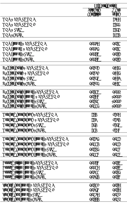
Table 4.1. Aggregate Volatility Indicators Results – Positive Price Shock

High price path Standard

deviation Mean value

GDP - ALT FUND 2 5299

GDP - FIEM 5385

GDP - BASE 5453

GDP growth - ALT FUND 2 0.0029 0.034

GDP growth - FIEM 0.0036 0.035

GDP growth - BASE 0.0036 0.035

Exchange rate - ALT FUND 2 0.0715 0.938

Exchange rate - FIEM 0.0786 0.932

Exchange rate - BASE 0.0718 0.934

Exchange rate growth - ALT FUND 2 0.0346 0.000

Exchange rate growth - ALT FUND 1 0.0397 -0.001

Exchange rate growth - FIEM 0.0504 -0.001

Exchange rate growth - BASE 0.0448 -0.001

Government revenue - ALT FUND 2 533 1519

Government revenue - FIEM 583 1586

Government revenue - BASE 543 1597

Government revenue growth - ALT FUND 2 0.0528 0.045

Government revenue growth - FIEM 0.0538 0.047

Government revenue growth - BASE 0.0447 0.046

Consumption growth - ALT FUND 2 0.0137 0.036

Consumption growth - FIEM 0.0244 0.038

Consumption growth - BASE 0.0203 0.037

Investment growth – ALT FUND 2 0.0341 0.039

Investment growth - FIEM 0.0429 0.041

(35)

This analysis highlights the trade-offs in achieving the many possible objectives in reducing volatility. The enhanced performance of the two alternative funds in reducing most of the aggregate volatility indicators comes at the cost of increasing the size of the fund, keeping a larger portion of national savings away from production use. For example, the size of the fund in scenario ALT FUND 2 reaches a level equal to 66% of annual GDP compared to a level of 20% using the FIEM. The estimated reduction in growth for the ALT FUND 2 averages 0.7% per year. Again, it is not possible in this framework to explicitly quantify whether this is a good choice, but the weight of available evidence suggests that it is.

The last aspect associated with a positive price shock that we analyze is the impact on producer prices in domestic currency. Table 4.2 indicates that the reduction in most of the macroeconomic volatility indicators, including the real exchange rate, does not necessarily translate into a reduction in producer price volatility. For the petroleum sector, the movement in the real exchange acts to buffer much of the change in prices in the absence of the stabilization fund. By putting in place the stabilization fund, we are effectively reducing the price smoothing capacity of real exchange rate movements. For the non-tradeable sector, we are reducing the real exchange rate shock, but also reducing the impact of increased domestic spending. The net result is greater volatility in domestic prices for the non-tradeable sector. The tradeable sector is the only sector that enjoys mildly reduced domestic producer price volatility due to the activity of the stabilization fund.

(36)

Table 4.2. Impact of Positive Price Shock on Producer Prices in Domestic Currency

Standard deviation Mean value

Petroleum producer price - ALT FUND 1 0.162 1.141

Petroleum producer price - FIEM 0.161 1.134

Petroleum producer price - BASE 0.171 1.138

Non-tradeable producer price - ALT FUND 1 0.048 0.957

Non-tradeable producer price - FIEM 0.048 0.961

Non-tradeable producer price - BASE 0.048 0.962

Tradeable producer price - ALT FUND 1 0.056 0.944

Tradeable producer price - FIEM 0.056 0.944

Tradeable producer price - BASE 0.056 0.944

Petroleum producer price growth - ALT FUND 1 0.0305 0.0139

Petroleum producer price growth - FIEM 0.0287 0.0138

Petroleum producer price growth - BASE 0.0230 0.0140

Non-tradeable producer price growth - ALT FUND 1 0.0135 -0.0044

Non-tradeable producer price growth - FIEM 0.0205 -0.0041

Non-tradeable producer price growth - BASE 0.0109 -0.0044

Tradeable producer price growth - ALT FUND 1 0.0321 -0.0024

Tradeable producer price growth - FIEM 0.0387 -0.0022

Tradeable producer price growth - BASE 0.0337 -0.0024

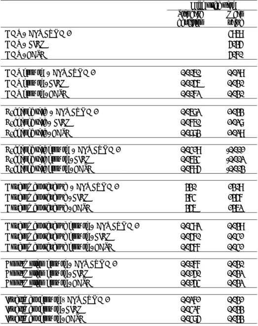
We now turn to the impact of the fund in the presence of a negative price shock. This is the more obvious context for expecting the stabilization fund to reduce volatility, as it should not only address the price fluctuations but also reduce the contractionary impact of the price drop. For this section, we drop the second alternative fund configuration, ALT FUND 2, because in the context of a negative price shock, it performs identically to ALT FUND 1. As can be seen in Table 4.3, both funds perform quite well in reducing the aggregate volatility indicators when faced with a negative price shock. ALT FUND 1 again out-performs the FIEM on all of the measures except GDP growth volatility. This is largely the result of a smoother transition path between deposits to and withdrawals from the fund.

(37)

Table 4.3. Aggregate Volatility Indicator Results – Negative Price Shock

High price path Standard

deviation Mean value

GDP - FIEM 5035

GDP - BASE 5070

GDP growth - FIEM 0.0056 0.030

GDP growth - BASE 0.0072 0.030

Exchange rate - FIEM 0.0760 1.028

Exchange rate - BASE 0.0883 1.029

Exchange rate growth - ALT FUND 1 0.0419 -0.001

Exchange rate growth - FIEM 0.0634 -0.002

Exchange rate growth - BASE 0.0795 -0.003

Government revenue - FIEM 374 1357

Government revenue - BASE 356 1362

Government revenue growth - FIEM 0.0570 0.041

Government revenue growth - BASE 0.0577 0.041

Consumption growth - FIEM 0.0150 0.032

Consumption growth - BASE 0.0154 0.032

Investment growth - FIEM 0.0427 0.033

Investment growth - BASE 0.0485 0.033

The impact of the stabilization fund on producer prices for a negative price shock displays ambiguous results, similar to the results of the positive price shock. In the petroleum sector, a freely floating exchange rate more effectively buffers domestic price movements than the actions of the stabilization fund. The stabilization fund smoothes movements in the tradeables sector domestic prices as they are linked to the real exchange rate. The results for the non-tradeable sector is more complex with price movements that are linked more closely to the activity of the fund in addition to the real exchange rate and the activity of the fund. In this context, the withdrawals from the stabilization fund