2008 A P P L IE D AN DN ATURAL SCIENCE F O U N D A T IO N ANSF
JANS
Journal of Applied and Natural Science 9 (3): 1666 -1675 (2017)
INTRODUCTION
It is assumed, for each sampling design, that the true values of the variables of interest could be made avail-able for the elements of the population under consid-eration. However, this may not be true particularly for large scale surveys. Errors can occur at almost every stage of planning and execution of a large scale survey. These errors may be attributed to various causes right from the beginning stage, when the survey is planned and designed, to the final stage when the data are col-lected, processed and analyzed. For large or medium scale surveys we are often faced with the scenario that the sampling frame of ultimate stage units is not avail-able and the cost of construction of the frame is very high. Sometimes the population elements are scattered over a wide area resulting in a widely scattered sample. Therefore, not only the cost of enumeration of units in such a sample may be very high, the supervision of field work may also be very difficult. For such situa-tions, two-stage or multi-stage sampling designs are very effective. It is also the case that, in many human surveys, information is not obtained from all the units in surveys.
Colombo (1992), Anido and Valdes (2000) and Biemer and Link (2006) proposed the call-back approach to reduce the nonresponse bias. The problem of non-response persists even after call-backs. The estimates obtained from incomplete sample data become biased. Hansen and Hurwitz (1946) proposed a technique for adjusting for non-response to address the problem of bias. The technique consists of selecting a sub-sample
of non-respondents and the data are collected through specialized efforts from the non-respondents so as to obtain an estimate of non-responding units in the popu-lation. Tripathi and Khare (1997) extended the sub-sampling of non-respondents approach to multivariate case. Okafor (2001, 2005) further extended the ap-proach in the context of element sampling and two-stage sampling respectively on two successive occa-sions. Chhikara and Sud (2009) used the sub-sampling of non-respondents approach for estimation of popula-tion and domain totals in the context of item non-response. Various authors have used auxiliary informa-tion to improve the estimate by developing ratio and regression type estimators in the presence of non-response. Notably among them are Rao (1986), Khare and Srivastava (1993), Khare and Sinha (2009), So-dipo (2010), Singh and Kumar (2011), Monika Devi et al (2014) etc. Okafor and Lee (2000), Kumar and Viswanathaiah (2014) and many others extended the approach to double sampling for ratio and regression estimation. Al Baghal and Lynn (2015), Anderson et. al. (2015), Burton et. al. (2015), Fahimi et. al. (2015) and Matei and Ranalli (2015) proposed different ap-proaches to deal with the problem of non-response. Most of the work is however, dedicated to uni-stage sampling in the presence of non-response. The present work is therefore initiated to develop the methodology for estimation of population mean in two-stage sam-pling under non-response with the following objec-tives:
To develop an efficient estimator of population mean in two-stage sampling under Deterministic Response
Estimation of population mean in two– stage sampling under a deterministic
response mechanism in the presence of non-response
Monika Devi
*and B. V. S. Sisodia
Department of Agriculture Statistics, N.D. University of Agriculture & Technology, Faizabad, (UP), INDIA
*Corresponding author. E-mail: [email protected]
Received: June 24, 2016; Revised received: April 17, 2017; Accepted: August 9, 2017
Abstract: In the present paper, we have considered the problem of estimation of population mean in the presence
of non-response under two-stage sampling. Two different models of non-response with deterministic response mechanism have been discussed in the paper. The estimators under two non-response models have been devel-oped by using Hansen and Hurwitz (1946) technique. The expressions for the variances and estimates of variance of these estimators have been derived. The optimum values of sample sizes have been obtained by considering a suitable cost function for a fixed variance. A limited simulation study has been carried out to examine the magnitude of percent relative loss (% RL) in standard error due to non-response. An empirical study with the real populations has also been carried out to assess the % RL in standard error due to non-response.
Mechanism.
To carry out empirical study with real data to examine the performance of the estimators.
MATERIALS AND METHODS
The estimators for estimation of population mean in two-stage sampling in the presence of non-response have been developed under two non-response models. It is assumed that the non-response is deterministic. Consider that a finite population U consists of N pri-mary stage units (psus) labeled 1 through N, and each psu comprises of M second stage units (ssus). Let yij
be the value of study character y pertaining to j-th ssu in the i - th psu, i = 1,2,……,N, j = 1,2……, M,. The objective is to estimate the population mean
We state the first non-response model referred to as Situation-1 as follows:
Situation 1: It is assumed that the psu(s) are divided
into two strata, i.e. (i) first stratum consisting of N1
psu(s) from where we do not get response at all, and (ii) second stratum consisting of N2 psu(s) from where
we do get partial responses from ssu(s), such that N = N1 + N2 . A random sample of n psus is drawn from N
by simple random sampling without replacement (SRSWOR). From each selected psu a sample of m ssus from M ssu(s) is drawn by SRSWOR. Let there be complete non-response from n1 psus. In the n2 psu
(n1 + n2 = n) mi1 ssus respond while mi2 ssus do not
respond, mi1 + mi1 = m . A sub-sample of hi2 units is
selected by srswor from mi2 and data are collected
through specialized efforts. Further, a sub-sample of h1 psus is drawn out of n1 psus and data are collected
through specialized efforts on each of m ssus in the selected h1 psus. Let n1 = f1h1 and mi2 = fi2hi2, i = 1,2,
….n2. It is further assumed that in n2 psu(s) there are
Mi1 responding and Mi2non-responding ssu units such
that Mi1 + Mi2 = M.
First, we define the following:
,
sample mean in i - th psu (i ϵ n1)
,
sample mean in i - th psu (i ϵ n2) psu corresponding to
the responsing ssu(s).
,
sample mean in i - th psu (i ϵ n2) corresponding to sub
-sample of non-responsing ssu(s).
∑
= = m j ij im y m y 1 1∑
= = 1 1 1 1 1 i i m j ij i m y m y∑
= = 2 2 1 2 1 i i h j ij i h y h y , , , , , , , , , where, , ,We, now, state and prove the following theorem.
Theorem 2.1: An unbiased estimator of is given
by
…. (1)
with variance of as
… (2) and unbiased variance estimator as
(3) Proof: By definition,
(
)
∑
= − − = N i iM b Y Y N S 1 2 2 1 1∑
= = M j ij iM Y M Y 1 1(
)
∑
= − − = 1 1 1 1 2 2 1 1 N i N iM bN Y Y N S 1 1 1 h n f =∑
= = 1 1 1 1 1 N i iM N Y N Y(
)
2 1 2 1 1∑
= − − = M j iM ij iM Y Y M S(
)
∑
=(
)
− − = 2 2 2 1 2 2 2 1 1 i i i M j M ij i M Y Y M S∑
= = 2 2 1 2 1 i i M j ij i M Y M Y(
)
− + + − =∑
∑
= = 2 1 1 2 2 1 2 1 2 1 1 2 2 2 1 1 1 1 1 y n y m y m m y h n n s n i h i m i h i im b i i(
)
∑
= − − = 1 1 1 1 2 1 2 1 1 h i h im b y y h s h∑
= = 1 1 1 1 1 h i im h y h y(
)
− − =∑
= 2 1 2 2 1 1 1 im m j ij im y my m s∑
= = m j ij im y m y 1 1(
)
− + − =∑
∑
= = 2 1 2 2 2 1 2 2 1 2 1 1 im h j ij i i m j ij im y my h m y m s i i(
−)
∑
−(
−)
= 2 2 2 1 2 2 2 1 1 i i i h j h ij i h y y h s∑
= = 2 2 1 2 1 i i h j ij i h y h yY
+ + =∑
∑
= = 2 2 1 1 1 2 1 1 1 1 1 1 n i h i m i h i im m y m y m y h n n y i i 1y
( ) ( ) ( )2 1 1 1 2 2 2 1 2 1 2 1 2 1 1 2 2 2 1 1 1 1 1 1 1 1 1 bN N i M i i N i iM N i iM b f S Nn N S f Mm M Nn S S f M m Nn S N n y V ∑ ∑ ∑ i = = = − + − + + − + − = ( ) ( ) ( ) ( ) ( ) 1 2 2 1 2 1 2 1 2 2 1 2 1 1 1 1 1 2 2 2 2 1 2 1 1 2 2 2 1 1 1 1 1 ˆ 1 1 1 ˆ 1 1 1 1 1 1 1 1 i h n b im im i i n h i i h bh im i i n V y S f s s n N n m M h M m m n f s f s s m M h m M n m n = = = = = − + − + − + − − + − − − ∑ ∑ ∑ ∑( )
+ + =∑
∑
= = 2 2 1 1 1 2 1 1 1 1 4 3 2 1 1 1 n i h i m i h i im m y m y m y h n n E E E E y E i i∑ ∑
= = = N i M j ij y MN Y 1 1 1
Where E4 represents conditional expectation of all
possible samples of size hi2 drawn from a sample of
size mi2 , E3 represents conditional expectation of all
possible samples of size m drawn from M, E2 refers
to conditional expectation arising out of selection of all possible samples of size h1 drawn from n1 while E1
refers to expectation arising out of all possible samples of size n drawn from a population of size N.
To obtain the variance, we proceed as follows: By definition,
where , , , are defined similarly as
, , , .
where,
Thus, by adding all the terms we obtain the required result.
Taking the expectation and simplifying we get,
and + =
∑
∑
= = 2 1 1 1 1 1 3 2 1 1 n i im h i im y y h n n E E E + =∑
∑
= = 2 1 1 1 1 1 n i iM n i iM Y Y n E =∑
= n i iM Y n E 1 1 1∑
= = N i iM Y N 1 1Y
=
( )
y1 V1E2E3E4( )
y1 E1V2E3E4( )
y1 E1E2V3E4( )
y1 E1E2E3V4( )
y1 V = + + + 1V
V
2V
3V
4 1E
E
2E
3E
4( )
2 1 4 3 2 1 1 1 b S N n y E E E V − =( )
(
)
2 1 1 1 4 3 2 1 Nn f 1SbN1 N y E E V E = −( )
+ − =∑
∑
= = 2 1 1 2 1 2 1 1 4 3 2 1 1 1 1 N i iM N i iM S S f M m nN y E V E E( )
∑
(
)
= − = 2 2 1 2 2 2 1 4 3 2 1 1 1 N i M i i i S f Mm M nN y V E E E ( ) ( ) ( )2 1 1 1 2 2 2 1 2 1 2 1 2 1 1 2 2 2 1 1 1 1 1 1 1 1 1 bN N i M i i N i iM N i iM b f S Nn N S f Mm M Nn S S f M m Nn S N n y V i ∑ ∑ ∑ = = = + − + − + − + − =( )
( ) ( ) ( ) ( ) ( ) 1 2 2 2 1 1 2 2 2 2 1 2 3 4 5 6 7 1 1 2 2 2 1 2 1 1 1 1 1 1 1 1 1 1 1 1 i N N N b b iM iM i i N i i M b i n f E E E E E E E s S S S N n m M N m M M N f S f S N Mm N n = = = − = + − − + − + − − − − ∑ ∑ ∑( )
(
)(
)
2 2 2 2 2 21
1
i Mi i iM imf
S
m
M
M
S
s
E
−
−
−
=
( )
2 2 1imS
iMs
E
=
( )
∑
=+
−
=
1 1 1 1 2 2 1 21
1
1
N i b iM bhS
S
NM
m
N
s
E
Where E7 represents conditional expectation of all
possible samples of size hi2 drawn from a sample of
size mi2, E6 represents conditional expectation of all
possible samples of size mi1, mi2 respectively drawn
from Mi1, Mi2 , respectively by keeping mi1, mi2, fixed.
Here Mi1, Mi2 denote the number of responding and non
-responding units in the population, E5 refers to
condi-tional expectation arising out of randomness mi1, mi2,
Mi1, Mi1, Mi2 ,. refers to conditional expectation of all
possible samples of size m drawn from M, E3 refers to
conditional expectation of all possible samples of size h1 drawn from n1, E2, refers to expectation arising out
of all possible samples of size n1, n2 ,drawn from N1,N2
keeping n1, n2,fixed while E1 refers to expectation
aris-ing out of randomness of n1, n2.
Let,
,
for ,
for
and
Substituting the estimated values in the variance ex-pression (2.2) we get the required estimate of V(ӯ1).
To determine the optimum values of n, m, and fi2 by
minimizing the expected cost for a fixed variance, we use the relation mi2 = hi2 fi2, i=1,2,…., n2. To achieve
this, consider the following cost function
where, C: Total cost; C1: Per psu travel cost; C2: Cost
per ssu for collecting the information on the study character in the first attempt; C3: Cost per ssu for
col-lecting the information by expensive method after the first attempt has failed for obtaining information It is envisaged that C3 will be higher than C1 and
sub-stantially higher than C2.
The expected cost in this case is,
To minimize the expected cost subject to fixed vari-ance consider the function.
(
)(
2)
2 2 2 2 2 1 1 ˆ i h i i im iM f s m m m s S − − + = 2n
2 1 2ˆ
im iMs
S
=
1n
2 1 1 1 2 2 1 1 1 1 1 1 ˆ im h i bh bN s M m h s S ∑ = − − = 2 2 2 2ˆ
i i h Ms
S
=
( ) ( ) ( ) ( )( )1 2 1 1 2 2 2 2 1 2 1 2 1 2 2 1 2 2 2 1 ˆ 1 1 ˆ 1 1 ˆ 1 1 1 ˆ 1 1 1 1 ˆ bN n i M i i n i im n i iM b b f S n n n S f m m n S M m n S M m n f n n s S i+ − − − − − − − − − − =∑
∑
∑
= = =(
)
+
+
+
+
=
∑
∑
= = 2 2 1 1 2 3 1 1 2 2 1 1 n i i n i iC
h
h
m
m
C
n
h
C
C
( ) + + + + = = ∑ ∑ = = 2 2 1 1 1 2 2 3 1 1 2 2 1 1 1 * N i i i N i i m f N Mf nM C M mM C N f N C N n C E C( )
{
1 0}
*V
y
V
C
+
−
=
λ
φ
During optimization we have substituted f2 in place of
fi2 for simplicity in calculations. To overcome the
problem arising due to simultaneous minimization of n, m, f1 and f2, we assume that n2 = f1h2 for making the
calculations simple. Thus minimization gives the opti-mum values as ,
,
where,
,
,
Special case of Situation 1: Here we consider the case
that a sample of n psus is drawn from N, within each selected psu a sample of m ssus is drawn by srswor design. This sample is divided into two parts n1 and n2.
Let there be complete non-response in the n1 psus, n1 + n2 = n. Let there be no non-response in n2 psus, further
a sub-sample of h1 psus is drawn out of n1 psus and
data are collected through specialized efforts on each of m ssus in the selected h1 psus. Let n1 = f1h1. Assume N = N1 + N2 where N1 and N2 are the number of psus in
the population representing the two non-response categories considered here.
1 1 1 2 1 1
2
4
a
c
a
b
b
m
opt=
−
+
−
2 2 2 2 2 2 22
4
a
c
a
b
b
f
opt−
+
−
=
∑
∑
= =
−
=
2 1 1 1 2 1 2 1 2 3 11
N i iM N i bN iS
M
S
N
M
C
a
−
=
∑
∑
∑
= = = 2 1 2 2 1 1 1 2 2 1 2 2 3 1 N i N i N i M i iM iS
N
M
S
iM
C
b
∑
=−
=
2 2 1 2 2 1 1 1 N i M iS
iM
N
C
c
∑
∑
= ==
2 2 1 1 1 2 2 2 2 N i N i i iM iM
M
S
M
C
a
−
=
∑
∑
∑
= = = 2 2 2 2 1 1 2 2 2 1 2 3 2 N i N i iM M i N i iS
S
M
M
M
C
c
i + + − =∑
∑
∑
∑
∑
∑
= = = = = = 2 2 2 2 1 2 2 2 1 1 1 1 2 1 2 2 2 1 2 1 2 2 2 3 2 N i N i N i N i iM N i i M i N i i iM i i M S M S M M N S M M M C b iIn this context, we state and prove the following theo-rem.
Theorem 2.2: An unbiased estimator of Ῡis given by
… (4) with variance
… (5)
An unbiased estimator of variance is,
… (6) where,
, while rest of the terms are defined earlier.
Proof:
where, E3 represents conditional expectation of all
possible samples of size m drawn from M, E2 refers to
conditional expectation arising out of selection of all possible samples of size h1 drawn from n1 while E1
refers to expectation arising out of all possible samples of size n drawn from a population of size N.
To obtain the variance we proceed as follows: By definition, where,
+
=
∑
∑
= = 2 1 1 1 1 1 21
n i im h i imy
y
h
n
n
y
−
+
−
=
∑
∑
= = 2 2 1 2 1 2 1 1 2 1 21
1
y
n
y
y
h
n
n
s
n i im h i im b( )
+
=
∑
∑
= = 2 1 1 1 1 1 3 2 1 21
n i im h i imy
y
h
n
n
E
E
E
y
E
+
=
∑
∑
= = 2 1 1 1 11
n i iM n i iMY
Y
n
E
=
∑
= n i iMY
n
E
1 11
( )
∑
==
n i iMY
E
n
11
∑ ∑
= ==
n i N i iMY
N
n
1 11
1
Y
=
( )
y
2V
1E
2E
3( )
y
2E
1V
2E
3( )
y
2E
1E
2V
3( )
y
2V
=
+
+
+ = N S V k n b opt 2 0 ( ) ( ) 2 1 1 1 2 1 2 1 2 2 1 2 1 1 1 1 1 1 1 bN N i iM N i iM b f S Nn N S S f M m Nn S N n y V + − + − + − =∑
∑
= = ( ) ( ) − − − + + − + − = ∑ ∑ ∑ = = = 1 1 2 1 1 2 1 1 2 1 2 1 1 2 1 1 2 1 1 1 1 2 2 2 1 1 1 1 1 1 1 ˆ 1 1 ˆ h i im bh n i im h i im b s M m h s f n n s s h n f M m n S N n y V(
)
(
)
1 2 2 2 1 2 2 2 2 2 1 2 1 2 1 1 1 1 1 1 1 1 1 i 1 N N N i b iM iM M bN i i i M N k S f S S f S f S N m M = = N= Mm N = + − + + − + − ∑
∑
∑
Thus, by adding all the terms we obtain the required result.
Taking the expectation and simplifying we get,
, , as defined earlier.
Where E4 refers to conditional expectation of all
possi-ble samples of size m drawn from M, E3 refers to
conditional expectation of all possible samples of size h1 drawn from n1, E2 refers to expectation arising out
of all possible samples of size n1, n2 ,drawn from N1,
N2, keeping n1, n2 fixed while E1 refers to expectation
arising out of randomness of n1, n2. Let,
and
Substituting the estimated values in the variance ex-pression (2.5) we get the required estimate of . To determine the optimum values of n, m, and f1 we
proceed as earlier, i.e. minimization of expected cost subject to fixed variance. The optimum values are determined in the same way as the previous estimator by minimizing the expected cost with respect to fixed variance.
The relevant cost function in this case is,
The various costs are defined here are same as defined earlier. The expected cost is,
( )
2 2 3 2 1 1 1 b S N n y E E V − =( )
(
)
2 1 1 2 3 2 1f
1
S
bN1nN
N
y
E
V
E
=
−
( )
+
−
=
∑
∑
= = 2 1 1 2 1 2 1 2 3 2 11
1
1
N i iM N i iMS
S
f
M
m
Nn
y
V
E
E
( ) ( ) 2 1 1 1 2 1 2 1 2 2 1 2 1 1 1 1 1 1 1 bN N i iM N i iM b f S Nn N S S f M m Nn S N n y V + − + − + − =∑
∑
= = ( ) ( ( )) ( )( )2 1 1 1 2 1 2 1 2 2 4 3 2 1 1 2 1 1 1 1 1 1 1 1 1 bN N i iM N i iM b b f S n N N S M m N S M m n N n f n S s E E E E − − − − + − − − + = ∑ ∑ = =( )
∑
=+
−
=
1 1 1 1 2 2 1 21
1
1
N i b iM bhS
S
NM
m
N
s
E
( )
2 2 1imS
iMs
E
=
( ) ( ) ( )(1 ) 2 1 1 2 1 2 1 2 2 1 2 1 ˆ 1 1 ˆ 1 1 1 ˆ 1 1 1 ˆ bN n i iM n i iM b b f S n n n S M m n S M m n n n f n s S − − + − − − − − − = ∑ ∑ = = 2 1 2ˆ
im iMs
S
=
2 1 1 1 2 2 1 1 11
1
1
ˆ
im h i bh bNs
M
m
h
s
S
∑
=
−
−
=
( )y2 Vm
h
C
m
n
C
h
C
C
=
1 1+
2 2+
3 1Consider the function:
The minimization gives the optimum values as
where,
Control situation: The following estimator was also
considered for efficiency comparison purpose. Here we assume that srswor sample of n psus is selected from N and within each selected psu a sample of m ssus is selected from M ssus. Data are collected through specialized efforts to obtain complete response, i.e. there is no non-response. Then we give the following Theorem 2.3
Theorem 2.3 The estimator
( )
+
+
=
=
1 1 3 2 2 1 1 1 *f
N
m
C
m
N
C
f
N
C
N
n
C
E
C
4 4 4 2 4 4 12
4
a
c
a
b
b
f
opt−
+
−
=
+
=
N
S
V
k
n
b opt 2 0 3 3 3 2 3 32
4
a
c
a
b
b
m
opt=
−
+
−
(
)
2 1 1 1 2 1 2 1 2 1 2 1 1 1 1 1 bN N i iM N i iM b f S N N S S f M m N S k + − + − + =∑
∑
= =
−
+
=
∑
= 1 1 1 2 2 1 1 1 3 2 2 31
N i iM bNS
M
S
N
f
N
C
N
C
a
(
)
∑
=+
=
2 1 2 2 1 3 1 1 41
N i iMS
m
mN
C
N
C
c
+ − + =∑
∑
∑
= = = 1 2 1 1 1 2 2 1 2 1 1 3 1 2 1 1 3 2 2 3 N i N i iM iM N i iM fS S f N C S f N C N C b
+
−
=
∑
∑
= = 1 2 1 1 2 2 1 2 1 1 1 3 N i N i iM iMS
S
f
f
N
C
c
+
−
=
∑
= 2 1 1 2 2 2 4 2 1 11
1
N b N i iMN
S
S
M
m
N
C
a
( )∑
∑
= = + − + − = 2 1 1 1 1 2 2 1 3 1 1 2 1 1 2 1 3 4 1 1 1 N i iM b N i iM S m mN C N C S N S M m N C b N( )
{
2 0}
*V
y
V
C
+
−
=
λ
φ
… (7) is unbiased of Ῡ, ith variance,
…(8) where S2b and S2iM are already defined, and unbiased
estimator of variance,
… (9) where
Proof: The proof of unbiasedness of the given
estima-tor and its variance and unbiased variance estimaestima-tor can be found in Cochran (1997), pp. 277-278.
The cost function in this case is, C = C1n + C3nm
where, C, C1, C3, have been defined earlier.
To obtain optimum values of n and mwe minimize the cost by fixing the variance. The optimum values are as follows,
and
Simulation study: A limited simulation study has
been conducted with real data to examine the relative merits of the proposed estimators ӯ1 and ӯ2 and in
comparison to the usual estimators ӯnm (without
non-response) in two-stage sampling. A design based simu-lation based on real data is carried out. The following criterion was used for assessing the relative perform-ance of these estimators:
The percent relative root mean square error (RRMSE), which is defined as,
Here, is the value of estimator ( , &
∑∑
∑
= = ==
=
n i m j n i im ij nmy
n
y
nm
y
1 1 11
1
( )
∑
=
−
+
−
=
N i iM b nmS
M
m
Nn
S
N
n
y
V
1 2 21
1
1
1
1
( )
∑
= − + − = n i iM b nm S M m Nn S N n y V 1 2 1 2 1 1 1 1 1 ˆ i ˆ θ θˆy
1y
2) of ( )in the i-th (i=1,……,L=1000) simulation run.
Further, the percent relative loss in standard error in & due to non-response as compared to stan-dard error of has been computed as follows:
and
,
where , and
are the empirical root MSE of the esti-mator ӯnm(usual two-stage estimator without
non-response), ӯ1 & ӯ2 (our proposed estimators),
respec-tively.
Here,
, and
with ӯ1(i)
and ӯ2(i) are the values of our proposed estimators ӯ1
and ӯ2 in the simulation run i(i=1,….,L).
In design based simulation study with real data, we used the data given in Appendix-B: The MU284 popu-lation (Sarndal et al (1992)). From the Appendix-B, the 1985 population (in thousands) with respect to munici-palities has been considered as study variable. There are in all 284 municipalities. To form the psu(s), the first 15 municipalities constitute the first psu, and then next 15 municipalities form the second psu and so on. Therefore, we get in all 18 psu(s) each consisting of 15 ssu(s). In our study we used 270 municipalities out of 284 and remaining last 14 municipalities were left. 1000 independent random samples of size 7 psu(s) out of 18 are drawn by using simple random sampling without replacement. For each selected psu 6 ssu(s) m = 6 out of total 15 ssu(s) are drawn by using simple
nm
y
θ
Y
1y
y
2 nmy
( )
( )
( )
( )
100
%
1 1 1×
−
=
y
MSE
y
MSE
y
MSE
y
RL
nm( )
( )
( )
( )
100
%
2 2 2×
−
=
y
MSE
y
MSE
y
MSE
y
RL
nm( )
y
nmMSE
MSE
( )
y
1( )
y
2MSE
( )
(
( ))
−
=
∑
= 2 11
L i i nm nmy
L
y
RootMSE
θ
( )
(
( ))
−
=
∑
= 2 1 1 11
L i iy
L
y
RootMSE
θ
( )
(
( ))
−
=
∑
= 2 1 2 21
L i iy
L
y
RootMSE
θ
( ) (
)
, 1 1 2 1 2∑
= − − = n i im b y y n s(
)
−
−
=
∑
= 2 1 2 2 11
1
im m j ij imy
m
y
m
s
+ − + = ∑= N S V S M m N S n b N i iM b opt 2 0 1 2 2 1 1 1 − =∑
∑
= = N i iM b N i iM opt S MN S C N S C m 1 2 2 3 1 2 1 1( )
100 ˆ L 1 ˆ RRMSE % 2 L 1 i 1 × − =∑
=θ
θ
θ
θ
random sampling without replacement. We also con-sider that 18 psu(s) are divided into two classes, i.e. N1
= 6 and N2 = 6, where N1 constitutes the class of
com-plete non-responding psu(s) and N2 constitutes the
partially responding class/complete response class of psu(s), i.e. (N1 + N2 = N). Again we assume that that
the sample of size n=7 is also divided into two parts: i.e. n1 = 3 and n2 = 3 , which comes from complete non
-response and partially response classes, respectively. From n1 = 3, we further draw a subsample of size 2 (h1
= 2) and we make use of each of the values of m ssu (s) in the selected h1 psu(s). In the n2 = 4 psu(s), mi1 =
3 ssu(s) respond while mi2 = 3 ssu(s) do not respond.
A subsample of h12 = 2 units is selected by SRSWOR
from mi2. Here n1 = f1h1 = 3 and mi2=hi2fi2=3. We
com-puted the values of ӯnm,ӯ1, and ӯ2 from one thousand
samples. The true population mean Ῡ has been com-puted to be 29.90. The percent relative root mean square error (%RRMSE), the percent of relative loss in standard error (%RL) have been computed for our pro-posed estimators ӯ1 and ӯ2.
These computed values are presented in the Table 1. It is obvious that making bias adjustment in case of non-response in sample surveys, we loose efficiency of the estimators to some extent (Hansen & Hurwitz 1946). It is evident from the results of the Table 1 that the %RRMSE of the ӯ1 & ӯ2 have increased to about
24 percent in comparison to about 21 percent of ӯnm
(without non-response). The percent relative loss in standard error has been found more (10.36%) in case of ӯ1 as compared to that of ӯ2 (7.80) which is on the
expected line because more sampling error is expected in situation-I than situation-II.
Empirical study: An empirical study using some real
populations has also been carried out to examine the loss in standard error of the estimate due to non-response. Four populations viz. (i) P75 (1975 popula-tion (in thousands)), (ii) P85 (1985 populapopula-tion (in thousands)), (iii) RMT85 (Revenues from the 1985 municipal taxation (in millions of kronor)) and (iv) REV84 (Real estate values according to 1984 assess-ment (in millions of kronor)) have been considered from the Appendix-B of Sarndal et al. (1992). There are in all 284 municipalities. To form the psu(s), the first 15 municipalities constitute the first psu, and then next 15 municipalities form the second psu and so on. Therefore, we get in all 18 psu(s) each consisting of 15 ssu(s). In our study, we used 270 municipalities out of 284 and remaining last 14 municipalities were left. For each population, we have considered N =18, N1
=6, N2 =12, M = 15, Mi1 = 9, Mi2 = 6, n = 6, n1 = 3, n1 = 3, m = 8, mi1= 4,5, mi2= 4,3, hi2 = 2, ,
5
.
1
&
2
2 2 2=
=
i i ih
m
f
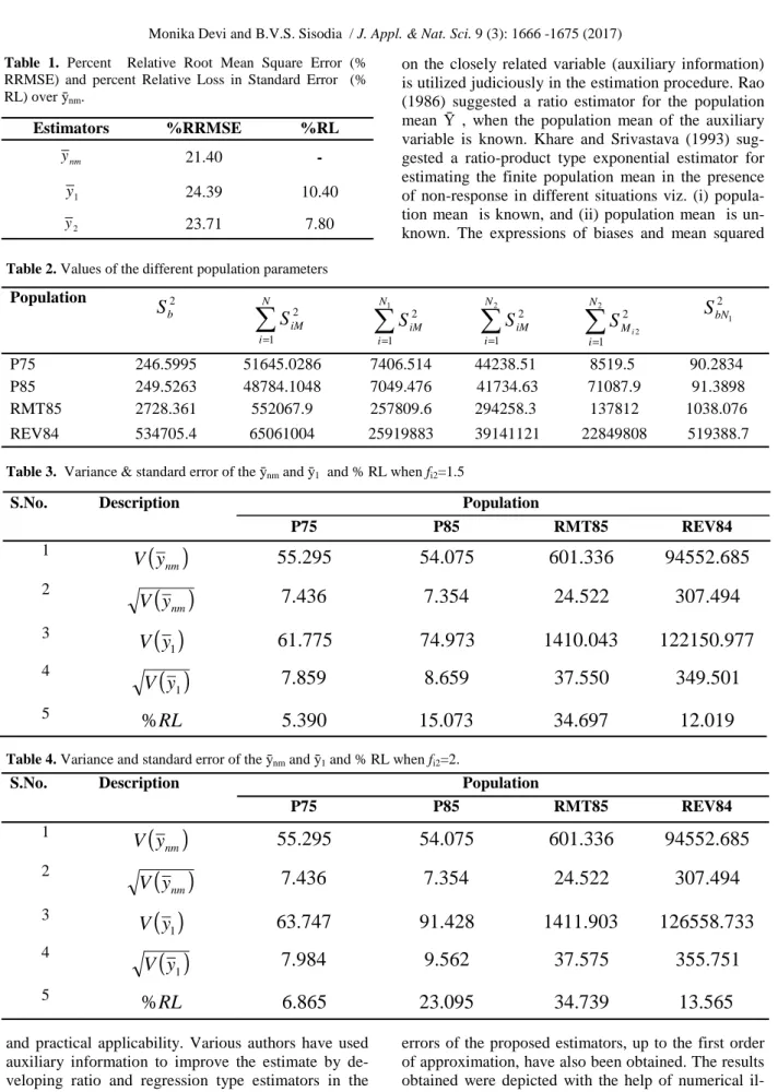
1.5 2 3 1 1 1 = = = h n fThe different population parameters involved in the variances of the estimators have been computed and are presented in the Table 2.
The variance of control estimator, i.e. V(ӯnm) has been
computed for each population. The variance of the proposed estimator ӯ1 for each population has been
computed for fi2 = 1.5 and 2.00. Similarly, the variance
of the proposed estimator ӯ2 for each population has
been computed for f1 = 1.5 .
The percent relative loss in standard error due to non-response over complete non-response with respect to the proposed estimators has been computed as follows
These results are summarized in the Table 3 to 5. It is obvious that making bias adjustment in case of non-response in sample surveys, we loose efficiency of the estimators to some extent (Hansen and Hurwitz 1946). It is evident from the results of the Table 3 and 4.3 that the percent relative loss in standard error has been found more in case of fi2 = 2 as compared to that
of fi2 = 1.5 for each population for the proposed
estima-tor ӯ1 over ӯnm. Since fi2 is the reciprocal of fraction of
sampled non-response ssu’s so in case of fi2 = 2 we
have more loss in percent relative standard error. So as the fi2 increases percent relative loss in standard error
also increases and it decrease with the decreasing value of fi2 for each population.
The Table 5 shows the percent relative loss in standard error in case of proposed estimator ӯ2 over ӯnm for
.
It is obvious that %RL will be less for proposed esti-mator ӯ2 for each population as compared to that of %
RL of estimator ӯ1 since estimator ӯ1 consists two
parts, one having complete non-response and, second of partial response whereas in case of estimator ӯ1 one
part has complete non-response and other has complete response.
It may also be noted that sampling rates and sub-sampling rates of respondent ssu(s) from non-respondents ssu(s) in selected psu(s) in the aforesaid simulation and empirical studies have already been at high side because of limitation of data. The de-crease in these rates would certainly increase the loss in efficiency.
RESULTS AND DISCUSSION
In order to make effective use of available sources various sampling technique have been developed from time to time which provide estimators of population characteristics of interest with high precision, reduced cost and above all will have the operational feasibility
5 . 1 1 1 1= = h n f
( )
( )
( )
100
,
%
=
−
×
i i nmy
V
y
V
y
V
RL
.
2
,
1
=
i
X X Xand practical applicability. Various authors have used auxiliary information to improve the estimate by de-veloping ratio and regression type estimators in the presence of non-response. It may lead to much im-provement in precision of estimation if the information
on the closely related variable (auxiliary information) is utilized judiciously in the estimation procedure. Rao (1986) suggested a ratio estimator for the population mean Ῡ , when the population mean of the auxiliary variable is known. Khare and Srivastava (1993) sug-gested a ratio-product type exponential estimator for estimating the finite population mean in the presence of non-response in different situations viz. (i) popula-tion mean is known, and (ii) populapopula-tion mean is un-known. The expressions of biases and mean squared
errors of the proposed estimators, up to the first order of approximation, have also been obtained. The results obtained were depicted with the help of numerical il-lustration. Singh and Kumar (2011) provided a Combi-nation of regression and ratio estimators in presence of
Table 2. Values of the different population parameters
Population 2 b
S
∑
= N i iMS
1 2∑
= 1 1 2 N i iMS
∑
= 2 1 2 N i iMS
∑
= 2 2 1 2 N i MiS
2 1 bNS
P75 246.5995 51645.0286 7406.514 44238.51 8519.5 90.2834 P85 249.5263 48784.1048 7049.476 41734.63 71087.9 91.3898 RMT85 2728.361 552067.9 257809.6 294258.3 137812 1038.076 REV84 534705.4 65061004 25919883 39141121 22849808 519388.7Table 3. Variance & standard error of the ӯnm and ӯ1 and % RL when fi2=1.5
S.No. Description Population
P75 P85 RMT85 REV84 1
( )
nmy
V
55.295
54.075
601.336
94552.685
2( )
nmy
V
7.436
7.354
24.522
307.494
3( )
1y
V
61.775
74.973
1410.043
122150.977
4( )
1y
V
7.859
8.659
37.550
349.501
5RL
%
5.390
15.073
34.697
12.019
S.No. Description Population
P75 P85 RMT85 REV84 1
( )
nmy
V
55.295
54.075
601.336
94552.685
2( )
nmy
V
7.436
7.354
24.522
307.494
3( )
1y
V
63.747
91.428
1411.903
126558.733
4( )
1y
V
7.984
9.562
37.575
355.751
5%
RL
6.865
23.095
34.739
13.565
Table 4. Variance and standard error of the ӯnm and ӯ1 and % RL when fi2=2.
Table 1. Percent Relative Root Mean Square Error (%
RRMSE) and percent Relative Loss in Standard Error (% RL) over ӯnm. Estimators %RRMSE %RL nm y 21.40 - 1 y 24.39 10.40 2 y 23.71 7.80
nonresponse. They addressed the problem of estimat-ing the population mean of the study variable y usestimat-ing information on two auxiliary variables x and z in pres-ence of nonresponse. Two classes of combined regres-sion and ratio estimators were defined in two different situations along with their properties. Many others extended the approach to double sampling for ratio and regression estimation.
Most of the work is however, dedicated to uni-stage sampling in the presence of non-response. Recently, Sud et al (2012) have made an attempt to develop the estimators of population mean in two-stage sampling in the presence of non-response. They have considered three types of non-response models. There are two more possible response models which they have not considered.
In what follows, we have considered these two non-response models for the development of the estimation of population mean in two-stage sampling design in the present paper. Here, we have considered the deter-ministic response mechanism. In situation-1, it is as-sumed that the psu(s) are divided into two strata, i.e. (i) first stratum consisting of N1 psu(s) from where we do
not get response at all, and (ii) second stratum consist-ing of N2 psu(s) from where we do get partial
re-sponses from ssu(s), such that N = N1 + N2. And in an
special case of situation-1, we assumed that the psu(s) are divided into two strata, i.e. (i) first stratum consist-ing of N1 psu(s) from where we do not get response at
all, and (ii) second stratum consisting of N2 psu(s)
from where we do get complete responses from ssu(s), such that N = N1 + N2. The expressions for the variances
and estimates of variance of these estimators have been derived. The optimum values of sample sizes have been obtained by considering a suitable cost function for a fixed variance.
Conclusion
The study of two-stage estimators of population mean under non-response has been presented. The optimum values of sample sizes have been obtained by consider-ing a suitable cost function for a fixed variance. It is
evident from the results of the Table 1 that the % RRMSE of the proposed estimators have increased to about 24 percent in comparison to about 21 percent of usual two-stage estimator (without non-response). The percent relative loss in standard error has been found more in situation-I as compared to that of situation-II which is on the expected line because more sampling error is expected in situation-I than situation-II. An empirical study using some real populations has also been carried out to examine the loss in standard error of the estimate due to non-response. It is also observed that the percentage relative efficiency decreases with increase in non-response. Since size of sub-sample is the reciprocal of fraction of sampled non-response
ssu’s so the percent relative loss in standard error will be more in case of small size sub-sample size as com-pared to that of a larger sub-sample and this has been supported by our empirical study results.
ACKNOWLEDGEMENTS
The present paper is a part of Ph.D. thesis of the first author, who is grateful to the DST, Govt. of India, for providing DST Fellowship (Inspire Fellowship) vide grant No. IF-120491 for carrying out present investiga-tion.
REFERENCES
Al Baghal, T. and Lynn, P. (2015). Using motivational state-ments in web-instrument design to reduce item-missing rates in a mixed-mode context. Public Opinion
Quar-terly, 79: 568 -579.
Anderson, Me., Henrikson, N., King, D. and Ulrich, K. (2015). Measuring the effects of operational designs on response rates and nonresponse bias. The American
Association for Public Opinion Research, 70th Annual
Conference. Retrieved from www.websm.org/ d b / 1 2 / 1 7 8 9 4 / W e b _ S u r v e y _ B i b l i o g r a p h y / Measurng_the_Effects_of_Operational_Designs_on_Re s p o n s e _ R a t e s _ a n d _ N o n r e s p o n s e _ B i a s / m e n u =1&lst=&q=search_1_111111_-1 & qdb=12 & qsort =1 Anido, C. and Valdes, T. (2000). An Iterative Estimation Procedure for Probit-type Nonresponse Models in
Sur-Table 5. Variance and standard error of the ӯnm and ӯ2 and % RL when f1=1.5
S.No. Description Population
P75 P85 RMT85 REV84 1
( )
nmy
V
55.295
54.075
601.336
94552.685
2( )
nmy
V
7.436
7.354
24.522
307.494
3( )
2y
V
59.803 58.517 1408.182 115980.118 4( )
2y
V
7.733 7.650 37.526 340.559 5RL
%
3.843 3.870 34.653 9.709veys with Call Backs. Sociedad de Estadistica e
Inveti-gacion Operativa, 9(1): 233-253.
Biemer, P., and M. Link (2006). “A Latent Call-Back Model for Nonresponse,” in 17th International Workshop on
Household Survey Nonresponse, Omaha, Nebraska,
USA.
Burton, J., Jaeckle, A. and Lynn, P. (2015). Going online with a face-to-face household panel: Effects of a mixed mode design on item and unit non-response. Survey
Research Methods, 9(1): 57-70.
Chhikara, R. S. and Sud, U. C. (2009). Estimation of popula-tion and domain totals under two phase sampling in the presence of non-response. Journal of the Indian Society
of Agricultural Statistics, 63(3): 297-304.
Cochran, W.G. (1997). Sampling Techniques, 3rd Edition. John Wiley & Sons, Inc., New York.
Colombo, R. (1992). Using Call-Backs to Adjust for Non-response Bias. Pages: 269-277. Elsevier, North Holland.
Fahimi, M., F. M. Barlas, R. K. Thomas and N. Buttermore (2015). Scientific Surveys Based on Incomplete Sampling Frames and High Rates of Nonresponse.
Sur-vey Practice, 8(5).
Hansen, M. H. and Hurwitz, W. N. (1946). The problem of nonresponse in sample surveys. Journal of the
American Statistical Association, 41: 517-529.
Khare, B. B. and Srivastava, S. (1993). Estimation of popula-tion mean using auxiliary character in presence of non-response. Nat. Acad. Sc. Letters, India, 16(3): 111-114. Khare, B.B. and Sinha, R.R. (2009). On class of estimators
for population mean using multi-auxiliary characters in the presence of non-response. Statistics in
Transition-new series. 10(1): 3-14.
Matei, A. and Ranalli, M.G. (2015). Dealing with non-ignorable nonresponse in survey sampling: A latent modeling ap-proach. Survey Methodology, 41(1), 145-164.
Monika, D., Sisodia, B.V.S. and Dube, L.K. (2014). Estima-tion of finite populaEstima-tion mean under non-response using auxiliary information. International Journal of
Agricul-tural and Statistical Sciences. 10(1): 127-131.
Okafor, F. C. and Lee, H. (2000). Double sampling for ratio and regression estimation with sub sampling the non-respondent. Survey Methodology, 26: 183-188. Okafor, F. C. (2001). Treatment of non-response in
succes-sive sampling, Statistica, 61(2):195-204.
Okafor, F. C. (2005). Sub-sampling the non-respondents in two-stage sampling over two successive occasions.
Journal of the Indian Statistical Association, 43(1): 33-49.
Rao, P. S. R. S. (1986). Ratio estimation with sub sampling the nonrespondents. Survey Methodology, 12(2): 217–230. S. Kumar and M. Viswanathaiah (2014). Population mean
estimation with sub sampling the non-respondents using two phase sampling. Journal of Modern Applied
Statis-tical Methods, 13(1): 187-198.
Sarndal, C. E., Swensson, B. and Wretman, J. (1992). Model Assisted Survey Sampling, Springer Verlag, New York. Singh, H. P. and Kumar, S. (2011). Combination of
regres-sion and ratio estimate in presence of nonresponse.
Braz. J. Probab. Stat., 25(2): 205-217.
Sodipo, A.A. (2010). Difference- type and regression- type estimators for the population mean based on post strati-fication and subsampling of the non-respondents.
Euro-pean Journal of Scientific Research. 43(4): 445-451.
Sud, U. C., Aditya, Kaustav, Chandra H. and Parsad, Ra-jender (2012). Two stage sampling for estimation of population mean with sub-sampling of non-respondents,
Journal of the Indian Society of Agricultural Statistics,
66(3): 447-457.
Tripathi, T. P. and Khare, B. B. (1997). Estimation of mean vector in presence of nonresponse. Communications in