THE EFFECT OF FEATURE COMPOSITION ON THE
LOCALIZATION ACCURACY OF VISUAL SLAM SYSTEMS
Mohamed Heshmat
and
Mohamed Abdellatif
Mechatronics and Robotics Engineering Department, School of Innovative Design Engineering, Egypt-Japan University of Science and Technology(EJUST), New Borg El Arab, Alexandria,Egypt
{mohamed.heshmat, mohamed.abdellatif }@ejust.edu.eg
Keywords: Monocular Visual SLAM: Feature Composition: Feature Selection Criteria.
Abstract: Simultaneous Localization and Mapping, SLAM, for mobile robots using a single camera, has attracted several researchers in the recent years. In this paper, we study the effect of feature point geometrical composition on the associated localization errors. The study will help to design an efficient feature management strategy that can reach high accuracy using fewer features. The basic idea is inspired from camera calibration literature which requires calibration target points to have significant perspective effect to derive accurate camera parameters. When the scene have significant perspective effect, it is expected that this will reduce the errors since it implicitly comply with the utilized perspective projection model. Experiments were done to explore the effect of scene features composition on the localization errors using the state of the art visual Mono SLAM algorithm.
1 INTRODUCTION
Simultaneous Localization and Mapping, SLAM is a fundamental problem in robotic research and there exist huge literature dealing with the problem from different perspectives and approaches.
Traditionally, SLAM exploits sensors that can measure the depth of scene objects directly such as laser range finders, ultrasonic range sensors or stereo camera range finders. Although sensors which measure depth explicitly always provide better accuracy of SLAM, the sensors are expensive and may complicate product marketing and user acceptance. Therefore, it is challenging to use a single camera that can infer the depth implicitly from its motion. Using visual information to solve the SLAM problem is intuitive, because human seems to do this and further more, robots are usually equipped with cameras.
The interest of using camera as the sole sensor for SLAM systems was active only recently because of the lack of robust techniques and the belief that it may be time consuming so that it may not work fast enough for real applications.
Feature-Based visual SLAM techniques find distinct visual features in the scene and track them among frames to recover camera motion and scene
map (Davison et al. 2007), (Jeong et al. 2006), and
(Lee et al. 2007).
The observed features in the scene can be thought of as a camera calibration target and when observed through the motion, we can obtain 3D reconstruction which constitutes a sparse feature map.
The best known solutions utilize either Extended
Kalman Filter, EKF (Davison et al. 2007), or
Particle filter (Eade et al. 2006). In this work,
Extended Kalman Filter, EKF, was used to solve the
SLAM problem from single video camera. (Civera et
al. 2008) devised one of the successful approaches
to solve the SLAM problem by using inverse depth parameterization. This parameterization solved the problem of representing distant points, with severe nonlinear effects due to the natural effects of depth. We adopt the inverse depth parameterization algorithm as implemented by (Civera et al. 2008). The point features used for solving SLAM were controlled based on their depth and the performance was explored.
The key question is whether all detected features will contribute equally to the accuracy of solving SLAM. Intuitively, we believe that the geometry of points affects the SLAM performance. Distant features contribute to the estimation of robot rotation angles but they are computationally expensive since they need to be represented in inverse depth with more parameters which slows down the SLAM algorithm. How much distant point features, and how much near point features are needed and useful is the question we try to answer in this paper.
Intelligence will impose the constraint that we have to select points that will only improve the accuracy and hence we can justify the added computational complexity, and consequently added processing time.
The objective is to find out selection rules of guaranteed beneficial feature points to the SLAM performance. This approach of feature management has not been considered before in the literature to the best of our knowledge.
The paper is arranged as follows: The next section outlines the EKF SLAM algorithm based on inverse depth parameterization. The experiments are presented in Section 3. Section 4 present the discussion and finally conclusions are given in Section 5.
2 EKF SLAM ALGORITHM
The Kalman Filter, KF, is a recursive Gaussian filter to estimate the state of continuous linear systems under uncertainty. The Extended Kalman Filter, EKF is an extension of the KF to model system non-linearities and detailed information on the Kalman filters and probabilistic methods can be found in
(Montemerlo et al. 2007), and (Thrun et al. 2005).
The state vector can be described as follows:
= r q v (1)
where r is the camera optical center position
referred to world reference coordinates, q refers
to the quaternion defining camera orientation; and
linear and angular velocity v and relative to
world frame W and camera frame C, respectively,
represents an appended dynamic vector of observed feature positions.
A constant acceleration is assumed in our state definition but the EKF will accommodate its changes as noise or disturbance. The dynamic model equations can be stated as follows:
= ∆∆ (2) = !" # !" $ !" !" % & '= + $+ ∆ #+ #+ ∆ $+ + % & ' (3)
where )* are linear and angular
acceleration, respectively, #+ ∆ the
quaternion of the rotation vector + ∆.
Here, the prediction is the standard for EKF, using the previous state vector and the dynamic model. The EKF update is done in two stages, one using low innovation inliers, and the other using
high innovation inliers (Civera et al. 2010).
In the inverse depth parameterization of 3D point, 6 elements vector is used to descibe features and can be defined by
+= ,-. /. 0. 1+ 2+ 3+4 (4)
This vector describes a ray whose optical centre
lies at (-+ /+ 0+ from which the point has been first
observed. 1+, 2+ are the azimuth and elevation angles
in the world frame, respectively, 3+ is the inverse
depth of the point along the ray. /+ represent 3D
feature through this equation:
+ = 6 -+ /+ 0+ 7 +31 +91+, 2+ (5) where
9 = cos 2+sin 1+, − sin 2+, cos 2+cos 1+ (6) The point observation can be represented as a ray from the camera to the point, expressed in the camera frame: ℎA= ,ℎB ℎC ℎD4 (7) ℎA= EAF G3 +GH -+ /+ 0+ I − FAJ + 91 +, 2+J (8)
The camera observes its projection in the image plane according to the camera pinhole model:
ℎ = K$ = KL− BℎℎB D $L− CℎℎC D% & ' (9)
where uL, vL are the image centre coordinate, and
fO, fP are the focal lengths measured along x, y
directions respectively. Because in the real world usually there is distortion, a distortion model has to
be applied (Civera et al. 2008, 2010).
3 EXPERIMENTS
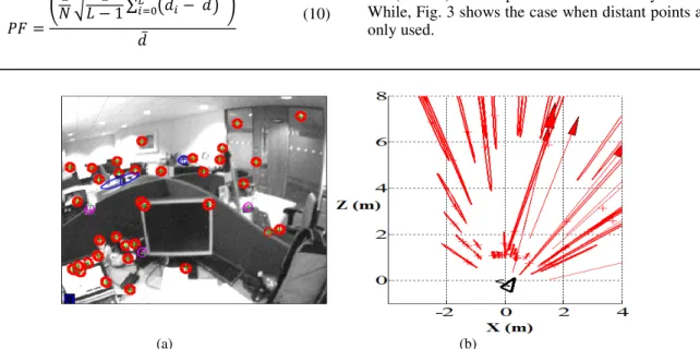
The code implemented by Civera, based on the inverse depth parameterization, is used throughout this work (Civera website. 2011) together with the dataset provided. Figure 1 shows the program interface, inside which a) shows a frame from the used data set and the detected features with colour circles overlaid on it, and b) shows the map and the camera motion.
In the code, the FAST corner detector is used to detect point features (Rosten and Drummond. 2006), but it is possible to use any other detector. The only constrain is to have plenty of features to select among them.
In camera calibration literature, features
geometric diversity is known to affect the calibration accuracy (Tsai. 1987). Therefore, viewing features as a dynamic calibration target, we intuitively expect that the same could have a similar effect on robot localization accuracy.
The feature diversity or composition is measured here in terms of what we call as the Perspective Factor, PF which is described by
QR =S1T U
1
V − 1 ∑ ,*Z+[L +− *̅4Y\
*̅
(10)
where N is the number of frames, L is the features
number, d` is the depth of the ith feature, and da is the
average depth. This value represents the standard deviation of features depth normalized by their average depth from camera.
Through the experiments the values of the perspective factor and the averaged sum of squared error, SSE of the robot position and orientation were computed.
The Perspective Factor values are controlled by removing some features, but with preserving the minimum number of features required in the experiment.
The case where the whole detected features is taken as a reference for our results, as we are concerned here with the relative relations not the
absolute accuracy of the results (Kummerle et al.
2009).
We controlled the scene features at first by selecting, two terminal cases, namely near features, and distant features. The near features are defined to be less than 3 meters in this case. On the other hand, the distant features are considered to be more than 7 meters. The position error in X, Z, and its’ uncertainty along the frames are registered. Also, The XZ motion of the camera is registered for each case.
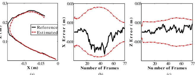
We examine the effect of selecting only the near or distant features on the accuracy of localization. Figure 2 shows the XZ path of the camera and the resulting errors and uncertainty in motion trajectory along the X and Z axes for near features, where the black (solid) line represents the error value and the red (dashed) lines represent the uncertainty bounds. While, Fig. 3 shows the case when distant points are only used.
(a) (b)
Figure 1: The program Interface, a) Sample frame of the test scene, and b) the camera motion and the detected features with uncertainty represented by ellipses in XZ plane.
As shown in Fig. 2, the near features give good results in terms of the error values and the convergence of the uncertainty. In contrast, as shown in Fig. 3 the distant points give large values of errors, and uncertainty divergence.
On the side of the XZ motion of the camera, the near points show good tracking of the reference path, but the distant points do not.
From this part of the experiment it is shown that, the near features have strong effect on the localization accuracy.
4 DISCUSSION
The localization error can be quantified by computing the difference between the reference
values and the estimated values of robot location or orientation through complete tour. This can be described by:
bc =T de1 fgh− eY
i j[L
(11)
where plmn is the reference parameter of position or
orientation and p is the estimated value.
Experiments are done using different values of the perspective factor. For each value of the perspective factors, the average sum of square errors
of the camera position and orientation (X Z o) are
computed.
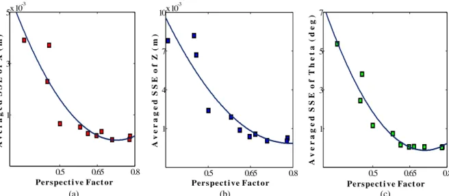
The effect of the perspective factor on the
averaged SSE in (X, Z, o) is shown in Fig. 4.
(a) (b) (c)
Figure 2: The camera path of experimental data set and associated localization error when using near features only. a) Camera motion path. The localization error (solid) and the associated uncertainty bounds (dashed) in b) errors of X-direction, and c) errors of Z-direction.
20 40 60 77 -0.01 0.01 0.03 N u m b e r o f F r a m e s X E r r o r ( m ) 20 40 60 77 -0.01 0.01 0.03 N u m b e r o f F r a m e s Z E r r o r ( m ) -0.3 -0.15 0 0.1 0.2 0.3 X ( m ) Z ( m ) R e f e r e n c e E s t i m a t e d (a) (b) (c)
Figure 3: The camera path of experimental data set and associated localization error when using distant features only. a) Camera motion path. The localization error (solid) and the associated uncertainty bounds (dashed) in b) errors of X-direction, and c) errors of Z-direction.
20 40 60 77 0 0.04 0.08 0.12 0.16 N u m b e r o f F r a m e s X E r r o r ( m ) 20 40 60 77 0 0.04 0.08 0.12 0.16 N u m b e r o f F r a m e s Z E r r o r ( m ) -0.4 -0.3 -0.2 -0.1 0 0.1 0.2 0.3 X ( m ) Z ( m ) R e f e r e n c e E s t i m a t e d
Table 1: The correlation coefficient between Perspective Factor and localization errors.
In the figure, each single point represents the error accumulated through the same tour for each value of Perspective Factor. The errors are shown for only these parameters since those are subject to main changes. An inverse relationship between them can be observed, when increasing the perspective factor, error values decrease.
Euclidean distance is a good measure of total deviation from reference path and was used for
representing the position errors (Funke et al. 2009).
Figure 5 shows the relationship between the perspective factor and the Euclidean error distance of averaged SSE in position (X, Z).
In general, by increasing the perspective factor, the errors are decreased. Therefore, we are advised to select among feature points (assuming we have plenty of points), the set of points which cause PF to have higher value.
Correlation Coefficient (R2) declares the strength
of the relation between two variables.
E2=
∑
-/ − )-a
/a
2∑
-2− )-a
2∑
/2− )/a
2(12)
Correlation Coefficient between PF and the
averaged SSE in (X Z o) were computed and its
values are shown in Table 1. The high values, shows strong correlation between PF and the errors values.
Parameters Correlation Coefficient, R2
Averaged SSE of X 0.8539
Averaged SSE of Z 0.8704
Averaged SSE of o 0.9427
This table confirms that Perspective Factor is a strong factor that limits the localization errors. Generally, to have higher localization accuracy, we should increase the perspective factor by proper selection of features.
(a) (b) (c)
Figure 4: The effect of the perspective factor on the localization errors measured in, a) X-direction, b) Z-direction, and c) o-orientation angular errors.
0.5 0.65 0.8 1 4 7 10x 10 -3 P e r s p e c t i v e F a c t o r A v e r a g e d S S E o f Z ( m ) 0.5 0.65 0.8 1 3 5 7 P e r s p e c t i v e F a c t o r A v e r a g e d S S E o f T h e t a ( d e g ) 0.5 0.65 0.8 1 3 5x 10 -3 P e r s p e c t i v e F a c t o r A v e r a g e d S S E o f X ( m ) 0.5 0.65 0.8 2 5 8 11x 10 -3 P e r s p e c t i v e F a c t o r E r r o r o f E u c l i d e a n D i s t a n c e
Figure 5: The effect of perspective factor on the Euclidean error distance of camera localization.
5 CONCLUSION
In this paper, the effect of features geometric configuration was studied on the SLAM algorithm performance using Civera inverse depth algorithm. A new factor was introduced, called the Perspective Factor, which expresses the degree of features depth variance normalized by features average depth from camera.
It was found that the localization error is highly correlated with the perspective factor. When features showed sufficient depth change compared to its mean depth from the camera, the estimation of the camera motion was more accurate because the feature geometrical content gave sufficient cues for the inference process.
Hence, selecting features points based on perspective factor is useful to reduce localization error when we have plenty of features in the scene to select from.
ACKNOWLEDGEMENT
The first author is supported by a scholarship from the Ministry of Higher Education, Government of Egypt which is gratefully acknowledged.
REFERENCES
Civera, J., Davison, A.J., Montiel, J.M.M., 2008. Inverse Depth Parametrization for Monocular SLAM. In IEEE Transactions on Robotics, 24(5): pp. 932–945. Civera, J., Grasa, O. G., Davison, A.J., Montiel, J.M.M,
2010. 1-Point RANSAC for EKF Filtering: Application to Real-Time Structure from Motion and Visual Odometry. Journal of Field Robotics, 27(5): pp. 609-631.
Civera website http://webdiis.unizar.es/~jcivera/code/1p-ransac-ekf-monoslam.html (accessed at 12:00 1/10/2011).
Davison, A. J., Reid, I. D., Molton, N. D., Stasse, O., 2007. MonoSLAM: Real-Time Single Camera SLAM. In IEEE Transactions on Pattern Analysis and Machine Intelligence, 29(6): pp. 1052–1067.
Eade, E., Drummond, T., 2006. Scalable Monocular SLAM. IEEE Conf. Computer Vision and Pattern Recognition, New York, Jun 17-22, vol. 1, pp. 469-476.
Funke, J., Pietzsch, T, 2009. A framework for evaluating visual slam. In Proc. of the British Machine Vision Conference.
Jeong, W.Y., Lee, K.M., 2006. Visual SLAM with Line and Corner Features. In Proc. of IEEE/RSJ Int. Conf. on Intelligent Robots and Systems, pp.2570-2575.
Kummerle, R., Steder, B., Dornhege, C., Ruhnke, M., Grisetti, G., Stachniss, C., Kleiner, A., 2009. On measuring the accuracy of SLAM algorithms. Autonomous Robots, 27(4): pp. 387-407.
Lee, Y.J., Song, J.B., 2007. Autonomous selection, registration and recognition of objects for visual SLAM in indoor environments. In the International Conference on Control, Automation and Systems. Montemerlo, M., Thrun, S., 2007. FastSLAM: A Scalable
Method for the simultaneous localization and mapping problem in robotics. In Springer Tracts in Advanced Robotics, vol. 27.
Rosten, E.,Drummond, T., 2006. Machine learning for high-speed corner detection. European Conference on Computer Vision.
Se, S., Lowe, D.G., Little, J., 2002. Mobile Robot Localization and Mapping with Uncertainty Using Scale-Invariant Visual Landmarks. International Journal of Robotics Research, 21: pp. 735–758. Thrun, S., Burgard, W., Fox, D., 2005. Probabilistic
Robotics. The MIT Press, Cambridge, Massachusetts, 3rd edition, pp. 39-81.
Tsai R., 1987. A versatile camera calibration technique for high—accuracy 3D machine vision metrology using of-the-shelf TV cameras and lenses. IEEE Journal of Robotics and Automation, 3(4): pp. 323-344.