doi:10.1093/climsys/dzx003 Advance Access Publication Date: 18 July 2017 Research Article
This Open Access article contains public sector information licensed under the Open Government Licence v2.0 (http://www.nationalarchives.gov.uk/doc/ open-government-licence/version/2/).
Published by Oxford University Press 2017.
Research Article
Towards the validation of a traceable climate
model hierarchies
Robin Tokmakian
a,*
and Peter Challenor
ba
Department of Oceanography, Naval Postgraduate School, Monterey, CA, USA and
bDepartment of
Mathematics, College of Engineering, Mathematics and Physical Sciences, University of Exeter, Exeter, UK.
*Correspondence Robin Tokmakian, Department of Oceanography, Naval Postgraduate School, 833 Dyer Rd, Bldg 232, Rm 328 Monterey, CA 93943, USA; E-mail: [email protected]Received 5 January 2017; Revised 5 July 2017; Accepted 11 July 2017
Abstract
Background. It is a common practice to use a simple model to explain the mechanisms or processes that occur in a much more complex, complete and computationally expensive model. Many such examples can be found in climate change research.
Objective. This paper uses two illustrative examples to show how we can quantitatively relate the mechanisms or processes observed in a simple climate model to similar mechanisms in a more complex one.
Method. A simple model can only explain a more complex solution’s mechanisms if outcomes are tested over a broad range of inputs. By carefully sampling the full set of inputs for both the simple and complex models, we can robustly compare the process or mechanistic outcomes, statistically, between them. Thus, by examining the similarity or differences in the relationship between the inputs and outputs. The method can reject an incorrect simple model.
Results. The examples are, first, analytic and numerical solutions to the heat equation and, second, the 1948 Stommel model of horizontal ocean circulation and a more complex quasi-geostrophic ocean model. We quantitatively state how similar the simple model’s mechanisms are to the mechanisms in the more complex representation. In addition, when a simple solution may be correct, we give the percentage of the variance of the complex model’s outcomes that is explained by the simple response along with an uncertainty estimate.
Conclusion. We successfully tested a methodology for robustly quantifying how the physics encapsulated by a simple model of a process may exhibit itself in another, more complex formulation. Suggestions are given as a guide for use of the methodology with more complex and realistic models.
1. Introduction
Various kinds of model hierarchies (Hoskins, 1983; Nikurashin and Vallis, 2012; Knutti and Rugenstein, 2015) allow us, to some degree, to explain responses in complex models in terms of physical processes encapsulated in simpler ones. While it is possible to argue, heuristically, which physical processes are important in a complex solution using a simpler model, such arguments do not quantitatively link the simple one to a more complex model. Furthermore, in contrast, as Knutti and Rugenstein (2015) suggest, if we want to argue that a simpler solution can represent key processes of a complex model, a quantitative analysis of the two models and their relationship to each other is neces-sary. Such a requisite, rigorous method should be able to understand how a simple model’s response space (and the physics within it) maps onto a similar solution space of the complex implementation.
Examples of quantifying connections within model hierarchies [In the broadest sense, a set of models that are hierarchical are ones in which the physics of the lower model are found in the higher, more complex model. The simple model is less computationally demanding than the complex model.] exist (Tran et al., 2016; Oughton and Craig, 2016), though not in the context of understanding physical processes or mechanisms that drive climate change. Quantifying such connections should provide us with confidence in our explanations and should help to distinguish between different possible simpler formulations of physical processes and their representation in a complex model. Such analysis can also allow us to rule out physical processes that are not present in the complex model. We propose a method that allows not only models of the same species [e.g. Community Earth System Model (CESM) at different resolutions] but also ones that are within the same general family [for example, conceptual models of ocean circulation and general circulation models (GCMs)] to be traceable [By traceable, we mean that the physics in the complex model can be attributed, quantifiably, to the physics of the simpler model. We also use mechanism and process, interchangeably, to refer to the underlying physics that control the dynamics (the move-ment of fluid, rather than in a mathematical sense of a dynamical systems) represented by the model.] from the simpler to the more complex model.
Using modern statistical machinery [Gaussian process (GP) emulators], we relate the response of the complex solu-tion to the response in the simpler model along with an associated uncertainty. This allows us to test whether a less complicated response, where we understand the physical mechanisms, is being reproduced (or not) in the complex model. The examples used in this paper have low computational requirements and could be addressed without emula-tors. Emulators become an important tool when the requirements to explore the input space of the complex model exceed the available computational resources. The key to success is the design of the experiment defined by a correct set of inputs to explain the outputs.
Two simple examples are used to explain this idea of tracing physical process through model hierarchies. The first is an abstraction. Our complex model is a set of partial differential equations solved numerically, and the simple model is the family of analytical solutions. We use this to illustrate the methodology. The second example is more real-istic and uses, as the complex model, a quasi-geostrophic (QG) model of the ocean with several parameters that can be varied. In this example, the simple physical process is a Stommel (1948) model of horizontal circulation, in which only bottom friction is allowed to change. Finally, we consider how this idea might be applied to hierarchies involving Climate Model Intercomparison Project (CMIP) class GCMs.
2. Methodology
The goal of this exercise is to show how to trace the physics from a simple and understandable model to similar physics in a much more complex solution with many more interactions and modelled processes and where it is not clear which physical processes are operating. The basic idea is that if the same physical processes are active in both the complex and simple models, then the response of the more sophisticated implementation to changes in the inputs (parameters) will be similar to the response of the simple model. Similarly, if the complex model does not respond in the same way to inputs as the simple model does, we can rule out these physical processes as being the driving force in the complex solution. We do not expect the response to be exactly the same, only similar.
We express this concept, mathematically, by considering, not only the relationship between the simple and complex solutions but also the difference between the simple formulation and the response from the complex model. That is:
= + +
x z x x z
where Yc is the model response from the complex implementation, a function of some vector of input parameters x (related
to the process or mechanism of interest) and a separate vector z (unrelated to the process of interest). Ys is the response
(out-come) from a simple model embodying the physical process. It is only a function of x. D is an additional response related to physical processes that are not accounted for by the simple model. It, also, is a function of the vector x and is unknown.
z
O( ) represents small-scale variability and other physical process contributions, which are unrelated to the inputs x but are a function of another, unspecified set of inputs z. Thus, we not only relate input quantities to outputs but also account for any differences in the two solutions that also can be related to the inputs. The success of this approach is that D( ) has to x
be distinguishable from O( )z. If there is no relationship between Yc and Y Ds+ , O( )z will be the dominant term.
The model is simple but encapsulates the question being addressed: does the complex implementation follow the simple dynamics or not? A more complex statistical model including, for example, interaction terms, could be built. Such a model would be difficult to fit. There may be problems with identifiability, but, more importantly, if we needed such a complex model, it would show that simple dynamics does not explain the behaviour of the complex model and hence answer our original question.
At its most fundamental level, the method we propose to use to trace the physical processes from a simple to a more complex model is a non-linear regression mapping of the set of inputs to the responses and to the dif-ferences between the simple and complex responses. In a larger context, these same methods are used to create statistical emulators to interpolate a limited set of model runs to give the full set of outcomes (and associated uncertainty) over the full range of input values. Furthermore, emulators have also been used in a variety of geo-physical problems and examples of their use are described in Higdon et al. (2004), Williams et al. (2006), Sansó et al. (2008), Sansó and Forest (2009), Hall et al. (2011), Tokmakian et al. (2012) and Tokmakian and Challenor
(2014). Alternative methods for statistically describing and analysing climate dynamics using Bayesian hierarch-ical models have been developed (e.g. Wikle et al., 2001). This work has mainly been involved with the assimila-tion of data and does not seem to map easily onto our problem. We have therefore not investigated such methods further in this context.
The first criteria for the success or not of this proposed approach is that the R2 value of the regression of the responses of the complex model versus the sum of the simple model responses plus the difference between the mod-els is significant and skilful. The outcomes should be tested for a broad range of input settings. The second criteria relates to the use of emulators. Because a physical model generally is expensive to run (e.g. GCM), an emulator can be employed to allow for the ability to create a set of outcomes from a broad set of inputs for the simple model, the complex model or both. The criteria for success for each emulator is that 90% of the validation cases fall within a 2σ uncertainty range of the mean emulator estimate for a given set of inputs.
A brief overview of the method is described next, with the details for those unfamiliar with GP emulators given in Appendix A. We develop the regression estimator or emulator using the assumption that the relationship between the inputs and outputs are smooth, but non-linear. Each of our models’ outputs will have a relationship such that
= x
Y F( ), where x is a vector of input parameter values, each with length q. Depending upon the problem, we create a sample set, Y, of a small size (n) of the model outcomes by one of two ways. The first is to specifically vary the inputs in both the simple and complex models in a similar manner so that the same physics is being modified. For example, varying a viscosity term in the examination of vertical mixing in the ocean. In some cases, especially in the realm of climate studies, the relationship between the inputs and the physical processes being studied may not be simple. For example, the influence of the Atlantic multi-decadal oscillation on the meridional overturning circulation does not relate in a simple way to a set of input parameters of an embedded process model. For such problems, some thought and care will be necessary to match inputs between the simple and complex implementations, possibly using sensitiv-ity analysis to identify the important inputs. The outcomes and inputs are then used to create emulators or regressions conditioned on the input vector x for the simple model, which we will refer to as Y ( )sx and for the difference, D( ).x
Formally,
≈ = +
x x x x
F( ) f( ) m0( ) G( ), (2)
where f is the regression function, m0 is some mean process function and G is a GP to capture the information that deviates from the mean. All are functions of the input vector x in which each element, x i( ), is the value for the ith par-ameter. An equation exists for each sample, j.
The prior specification of the regression function is an important part of specifying the emulator. In spatial statistics that use similar methods in a low dimension setting, there has been much discussion of confounding (see for example Hanks et al., 2015). However, in emulation, an efficient predictor of the underlying dynamical model is built, which we carefully validate. Because we are not interested in the form of the relationship in terms of the input variables, confounding is not an issue and we can use either simple prior mean functions, as used here, or more complex ones.
The GP regression interpolates the true outcomes Y at the locations where the simulator was run or sampled, which we will call the set Y, (also called the set of design locations). At other points, f ( ) gives an expected value x
for F( )x, the true function, along with an associated uncertainty estimate. A GP is used to determine f ( ) under the x
assumption that the uncertainty in the regression can be described with such a process. A GP can be understood as a generalization of a Gaussian distribution over an infinite vector space. Just as a Gaussian distribution has a mean and variance, a GP has a mean function and a covariance function. It does not mean that either the distributions of the inputs or the outcomes are Gaussian. Normally, the function F is smooth and continuous over its input space, although anything known about the outcome can be incorporated into the regression through the mean function. This can include strong non-linearities and discontinuities. With such a model, the uncertainty in the outcome, Y, at some vector location, x, is easily obtainable. Standard GP regression interpolates the data. If we add a ‘nugget’ term (an independent and identically distributed Normal random variable), the regression function no longer interpolates exactly (Gramacy and Lee, 2010; Andrianakis and Challenor, 2012).
Extensions to the standard GP methods have been developed which analyse hierarchies of models (see for example
Goldstein and Rougier, 2009). Assuming that there is a set of related models defined for various ‘levels’ t (e.g. resolu-tions, complexity) such that ys=f ( )sx, where f ( )sx is the emulator function for the simple model and ys is the approxi-mation of the output for the simple model. We also define the yc( )x =r Ys s( )x +d( )x, where d is a GP of the misfit (in
essence, a regression of the misfit, Y Yc− s) between the two model levels. It is only a function of x and rs is a set of
regression coefficients. yc is, then, the approximation for the complex model. The details can be found in Kennedy and O’Hagan (2000). The UK RAPIT Group (Williamson et al., 2012) used two related models of HADCM3 and a reduced resolution model FAMOUS, which has the same basic physics, to illustrate how the simpler implementation could make good predictions of the more complex model. Others, for example Tran et al. (2016), use such methods to have an inexpensive emulator replace an expensive model component of a climate system.
We test the validity of our regressions (emulators) by either using some additional input points (often chosen at random), or using known outcomes (Bastos and O’Hagan, 2009; Challenor, 2013). This is only advised when the numerical solutions or simulations are relatively cheap to run. In most cases, because the numerical solutions/ simulations are expensive to run, we test them by creating a series of emulators using only n 1− inputs and out-comes, leaving out each point in turn. The pair of inputs/outcomes that was not used in the emulator is then used to evaluate the validity of the regression, the ‘leave one out’ strategy. If 90% of the tests are successful, then we are confident the regression using the whole set of inputs and outcomes will be reasonable.
3. Example 1: heat equation
To illustrate our approach, we begin with an example using the heat equation. Our complex model is a numerical simulation of the equation, while the simple solution is the analytical solution. Two cases are provided. In the first case, the analytic solution is the correct solution for the heat equation, while in the second case, we test our method using an incorrect analytic solution.
The heat equation is defined as follows:
∂ ∂ = ∂∂ T t K T z 2 2 (3)
with the boundary conditions T(0, ) 0, ( , ) 0t = T Z t = , where Z 20 is the total depth, T is the temperature, t is time, z =
is depth and K is the diffusion coefficient. As the initial condition for the first case, we set T z( , 0)=Asin( )πZz, where A is a scaling coefficient. We now have two parameters, A and K, which we can vary resulting in a response T for every combination of the two parameters. The input vector x contains the values of A and K used to produce some response
We set up the first case such that we sample across a range of values (A = 1–10, K = 0.4–1) using a Latin hypercube (McKay et al., 1979) resulting in 100 (n) values for A and K that make up an input vector x1. We sample the solu-tions at z 3.8, and = t 24 giving us a vector of Y= s and Yc values, respectively, each vector of length 100. Using the set of inputs and the analytic solutions Ys, we create a regression or emulator (ys) as described in section 2 to represent the relationship between the inputs and outputs. We validate the regression by using 100 values of A and K chosen randomly. Figure 1a illustrates the results. We plot the emulator estimate of the outcome or response on the x-axis versus the true numerical outcome on the y-axis. The grey bars represent the uncertainty in the emulator outcomes (±2 SD). Ninety-nine of the 100 random values are within 2 SD of the given numerical value, giving an 99% signifi-cant level. Thus, we conclude that our regression ys for T for our analytic model is valid, within the given range of A and K values.
The second step in creating a traceable model hierarchy is to create an emulator or regression for the difference between our analytic and numerical model outcomes (Y Yc− s conditioned on x1). This regression or emulator is also validated by using the same random points as was done for ys. The results in Figure 1b show that the estimate of the differences and true difference both have values close to zero, with uncertainty on the order of 10e-3. This is as expected because the numerical model is close to an exact analytic solution (in other words, O( )z is approximately zero). The result is confirmed by Figure 1c, which shows the sum (yc) of the ys and d as compared to the true outcome of the numerical model, Yc. For this case, ys almost fully explains Yc because O( ) is zero and z d( )x1 is almost zero.
Our second case is an illustration of when the dynamics of a simple solution does not explain the outcomes of a more complex model. For this example, A is a value between -1 and -10 and K is a constant (5), giving us the set of inputs x2. We create a regression (ys) to relate these new inputs, x2, to the analytic outcomes Ys. Figure 1d
Figure 1. Example 1 Case 1: (a) Regression model, ys, versus true response of analytic solution, Ys, varying both A and k; (b)
regression, d, versus true difference, Yc−Ys, varying both A and k in both models; (c) regression, yc, versus truth Yc. Case 2: (d)
Regression model ys versus true response of analytic solution, Ys, varying only A; (e) regression, d, versus true difference, Yc−Ys,
varying only A in Ys and varying A and k in Yc. The regression is conditioned only on A; (f) regression model, yc, versus truth Yc,
with yc conditioned only on A. The circles represents the mean value from the regression model at 100 randomly sampled values
are the results, as expected, an almost perfect relationship between Ys and its associated regression, ys. Following the same steps as in Case 1, a regression, d( )x2, is created for relationship between the newly defined inputs (x2) and the difference between the analytic outcomes, Y ( )sx2, and the numerical set of solutions as defined in Case 1, Y ( )c 1x . Because 32 of the 100 emulator outcomes from our set of 100 random inputs fall outside 2 SD, as
seen in Figure 1e, we conclude that d( )x2 is not a good regression. Furthermore, a comparison of Y ( )c 1x (y-axis)
to the sum of y ( )sx2 and d( )x2 gives very low R2 value of 0.36, indicating that Ys does not represent the same process as given by Yc, even if we include some additional process, d, conditioned on x2. This leads to the conclusion, correctly, that in Case 2, the numerical solution does not follow the same response as found in the analytical model.
4. Example 2: Stommel model and QG model
Having illustrated the method using a relatively simple example, we now turn to a more complex problem. We will use, as our simple implementation of a process, the Stommel (1948) model of horizontal ocean circulation in a closed basin on a beta plane with bottom friction.
ττ ψ β β ψ ∂∇ ∂x = ∇ × + ∇ k 1 2 (4) where ∇ ×ττ represents the wind (τ) forcing of the system and βk is related to bottom friction. β is related to the Coriolis parameter and is constant for this problem.
The complex implementation will be a QG model (Pedlosky, 1996). The equation for the time-evolving stream function is given as follows:
ψ ψ ψ ψ µ ψ ψ ∂∇ ∂ + ∇ + ∂∇ ∂ = + ∇ + ∇ t J( , ) x we E 2 2 2 4 (5) where ψ is the streamfunction, ϵ is a coefficient related to advection, we is the vertical Ekman velocity associated with some forcing at the surface and E=βA
L
H
3 is a coefficient related to eddy viscosity. AH is the eddy viscosity coefficient, β is related to the Coriolis term and L is the width of the basin. The coefficient, µ=βrL, is the Stommel coefficient related to the bottom friction, r. J( ,ψ ∇2ψ) is the Jacobian of the stream function. The model will be examined when it reaches
steady state, and therefore, the first two terms are unimportant for our problem.
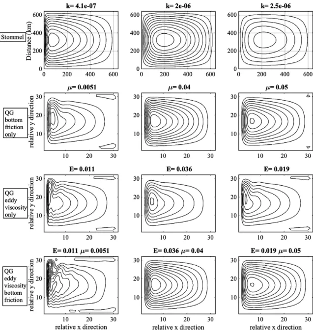
Physically, we would like to show how the Stommel model is represented in a QG formulation, especially in consideration that there are, most likely, interactions occurring between the bottom friction term and the eddy viscosity term as represented by the horizontal streamlines. Figure 2 presents the horizontal stream line fields for a subset of bottom friction and eddy viscosity parameter values. The three QG versions are as follows: row 2: varying only the Stommel related coefficient (μ), varying only the eddy viscosity term, E, and row 3: varying both of these terms. Each column represents a different location in the E, μ space. In general, the circulation, as shown by the streamlines, shows a circular pattern, with an enhanced western boundary current on the left side of each subplot. (Streamline values are relative, with the highest value in the centre and weakest value around the outside.) By eye, one might say that the Stommel solution (top row) is represented in all three versions of the QG model (rows 2, 3 and 4).
For each case below, we follow the same steps as in Example 1, that is (i) create an emulator for the simple solution, given a designed set of inputs, x (length of vector q 1) and outputs, Y= s, (ii) create an emulator for the difference in outcomes between the simple and the complex formulations and (iii) compare the resulting emulated outcomes, ys to see how well the simple model represents the processes in the complex implementation. Our input space, x, will be sampled from possible values of μ (or k in the Stommel model). The outcomes will be the stream-line value at yaxis=15 and xaxis=10 in the western portion of the domain near the point of the strongest flow. All
inputs and outputs are standardized before the regression or emulator is created. For our cases, 150 points (n) were sampled across the input space of the QG model using values of E and μ between 0.01 and 0.05 and for the Stommel model, k values between 0.4e-6 and 2.5e-6. The sampling of all parameters was determined by the same Latin Hypercube.
The results are given below. In Case 1, only the bottom friction parameter is varied in the QG model; in Case 2, only the eddy viscosity parameter is varied; and in Case 3, both the eddy viscosity parameter and bottom friction parameter are varied. In each case, we validate the emulator results in two ways. First, the emulator is validated by a ‘leave one out’ strategy. A second validation method can only be used when the simulator is cheap to run. This requires a sufficient size sampling of random input values to be used as inputs to the emulator and to the simulator. The outcomes from the emulator and the simulator can then be compared directly.
Figure 2. Plan view of stream function for a northern hemisphere basin. Top row: Stommel model with three different values of
bottom friction coefficient, k; second row: QG model with only the bottom friction coefficient (E) varied; third row: QG model varying only the eddy viscosity coefficient (μ); bottom row: QG model varying both the bottom friction and eddy viscosity terms. Streamlines are relative, with highest value as the centre ring and lowest value as the outside ring.
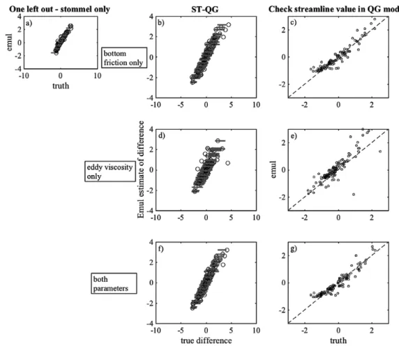
In Case 1, as we expect with only one parameter as an input (the bottom friction), we have a linear relationship between the emulator estimates (ys) of the streamline and the streamline value from the Stommel model (Fig. 3a), with small uncertainty. The emulator, or regression, of the difference between the Stommel and the QG outcomes (d), given a set of bottom friction values is also respectable with low uncertainty (Fig. 3b). For the second validation, the sum of the two emulators, ys and d, should compare favourably the true value of the QG simulator at the sampled input locations (Fig. 3c). The R2 estimate, y
c as compared to the truth Yc, is 0.99, allowing us to state with confidence that, indeed, the Stommel model is represented in the QG model response. This is expected, since the QG model at steady state reduces to the Stommel model if the eddy viscosity coefficient is held constant. Although unlike in the first example, the difference term, d( ) is not zero. We can say that the QG implementation is following the same physics x
as the simpler Stommel model but the response is not identical.
For Case 2 (Fig. 3d and e), when only the eddy viscosity coefficient, βALH
3, is varied and the bottom friction term is zero, the emulator of the difference, d, between the Stommel and the QG outcomes has a much larger uncertainty and 11 of the 150 ‘leave one out’ validity tests produce outcomes that are outside the range of uncertainty (52%). This is an acceptable emulator with a 93% confidence value, but with wide uncertainties (grey bands). However, where a
Figure 3. Example 2, input, x, is a set of bottom friction coefficient values, r or μ. The models’ responses, Yc and Ys, are the
stream-line values located at 0.5L (y-axis) and 0.3L, where L 600≈ for Stommel model and L 32= for QG model. Case 1: (a) Regression of Stommel model (ys) versus true values (Ys); (b) regression of difference d (Stommel model - QG model) conditioned on x; (c)
regression yc versus QG model with only bottom friction varying (μ). Case 2: (d) Same as (b), expect only eddy viscosity coefficient, E, varied in Yc, and regression conditioned on x containing varying values of bottom friction (μ); (e) same as (c), Yc only varied E.
Case 3: (f) Same as (b), but eddy viscosity (E) and bottom friction coefficients (μ) varied in QG model; (g) same as (c), except that eddy viscosity, E, and bottom friction coefficients, μ, varied. The circles represent the mean value from the regression model, while the grey line is the uncertainty in that estimate.
set of independent sampled values, Figure 3e, with the emulated streamline values are plotted versus the true values from the QG model, the R2 equals 0.52. The conclusion is that the physical processes in the simulator can not be represented by a simple model with only varying bottom friction.
Case 3 (Fig. 3f and g) is the most realistic of all the examples as we are varying both the eddy viscosity term and the bottom friction term in the QG model. The terms interact such that the response is non-linear in nature. As such, it illustrates a case in which a climate GCM contains many more processes than a simpler formulation of a process contains. Again, we have both an emulator of the streamline outcomes from the simple implementation (the Stommel model), ys, and an emulator of the difference, d, between the streamline values of the Stommel and the QG models. As Figure 3f illustrates, the emulator of the differences does a fairly good job of representing the outcomes of the differences (16 of the 150 values fall outside of 2σ or 90% confidence level). The uncertainty bands (given by the grey lines in the figure) are much smaller than for Case 2. A regression between the true differences and the emulated differences gives an R2 value of 0.99. This is confirmed by Figure 3g using a test of a set of 150 validation points that gives an R2 value of 0.98. It can be confidently stated that the dynamics of the Stommel model are represented in the QG model.
5. Example 3: time and space dilemma for geophysical flows
Complicating the analysis of geophysical flows is the high degrees of freedom (both in time and space) for such prob-lem. In the second example, the outputs of the Stommel and the QG models were sampled at one location. While the emulated solution and comparison of the two models is an adequate analysis at one location, the following question arises: does the solution hold for all locations? If the answer is yes, such a solution would give more weight to the justification that the simple model explains to processes in the complex model. It is possible to address this question just by creating an emulator for each location or a subset of locations as suggested by Rougier (2008). Depending on the size of the problem, this approach may be time consuming. It also does not address how the outcome of a process in one location relates to another location. A much simpler and elegant solution is to treat the spatial and temporal locations as additional input parameters. Just as the process parameter space is sampled broadly, the additional parameters, x and y, can also be sampled. In geophysical space, processes at a location are generally highly correlated with its near neighbours, thus making this approach attractive.
In this third example, the models from the second example are used, but now the x and y spatial locations are treated as input parameters in the creation of the emulator (q the length of the vector β is 3). And, rather than just sampling one location, as in Example 2, the outcomes of the Stommel and QG models are sampled at different x and y locations with every new setting of the bottom friction or eddy viscosity parameters. In other words, just as the models are not run at every bottom friction or eddy viscosity value, the x y, space does not need to be sampled everywhere. Again, three cases are run for the QG model: (i) varying only the bottom friction parameter, (ii) varying only the eddy viscosity term and (iii) varying both the bottom friction and eddy viscosity parameters. The result, shown in Figure 4, illustrates that the addition of the spatial parameters increases the confidence of the emulator for the first and third cases over just using one location (Fig. 4c and g), with R2 values of 0.92 and 0.91, respectively. For the case in which only the eddy viscosity term is varied, the R2 value is 0.76, For completeness, the validation (using the ‘leaveone out’ strategy) results in a valid emulator 97% of the time for Case 1, 93% of the time for Case 2 (but with wider uncer-tainty) and 97% of the time for Case 3. In summary, this third example illustrates how high spatial and temporal dimensions might be addressed successfully.
6. Discussion and conclusions
In the above examples, we have shown how one can use a statistical method to trace the dynamics of a rela-tively simpler model to the dynamics of a model with more complexity. The models may or may not be models within the same family (e.g. CESM models of differing resolutions). We acknowledge that climate GCMs are orders of magnitude more complex than these examples and care needs to be taken in how the inputs are chosen and which climate metrics are suitable to be used in this sort of problem. The following guidelines are proposed.
1. The input parameters need to be defined such that a wide range of values are allowed so that responses in the simple and complex models are variable. For example, the amount of CO2 (an absolute or percentage) applied as a forcing or the strength of the wind (related to CO2 uptake in the ocean).
2. Inputs and model responses should, each, be describing comparable physical processes in the simple and complex models.
3. The metric or model response should have a signal distinguishable from noise.
4. The inputs should be appropriate to the problem. For example, while the eddy viscosity coefficient is relevant for understanding whether or not an ocean model exhibits Munk theory circulation behaviour; on its own, the par-ameter will not help us in understanding the climate signal in complex GCMs. For the climate problem, we might chose a parameter such as the depth of the mixed layer for evaluating the amount of carbon uptake.
5. Metrics of a single variable or a spatial variable can be considered, and examples of both have been provided. A broad sampling of the output is an important to accurately reflect variations in the dynamics.
6. Section 2 states that the inputs x and z need to be clearly separable. It is possible to examine how parameters affect a process and for what range of values by exploring the full parameter space, as in this example from
Williamson et al. (2013). This initial step would identify regions of the input space x that is distinct from z for a given process in the complex model.
7. If a large number of possible dynamics are compared using these methods, the usual problems of multiple simul-taneous statistical tests will arise. We recommend the method is only used to compare small numbers of possible simple dynamical models.
8. We have deliberately simplified our methodology for clarity. In particular, in practice, we would use more sophis-ticated space-filling designs; maximin Latin hypercubes of even sequential designs.
Figure 4. Example 3, input, X, is a set of bottom friction coefficient values, r or μ, and spatial location x,y. The three cases are the same as Figure 3, but with the added inputs of a location in x y, space.
There are numerous climate-based problems that would be appropriate for such an analysis. One example is illus-trated in the following paper. Knutti and Rugenstein (2015) describe the qualitative relationships between outcomes from the complex CESM and a model of intermediate complexity, the ECBilt-CLIO model. CESM simulations with 4× CO2 forcing were compared with ECBilt-CLIO simulations using a range of forcings between cooling and 16× CO2. In their figure 9, they illustrate the relationship between surface temperature and top-of-atmosphere radiative imbalance with respect to how much CO2 forcing was used. Clearly, the relationship between the surface temperature and the top of the atmosphere (TOA) radiative balance is similar, but not the same between the CESM and the ECBilt-CLIO solutions. As described in this paper, to understand whether the same mechanism is functioning in both models, a few more simulations of CESM varying the CO2 forcing would be necessary to fully explore the response surfaces of the CESM and ECBilt-CLIO modules and their similarities. The next step to justifying this methodology would be to expand the method to more complex situations such as the example just described.
We have presented a methodology for robustly quantifying how the physics encapsulated by a simple model of a process may exhibit itself in another, more complex formulation. The method conclusively rejects simple phys-ical process models that do not have the same pattern of variation as the physics of the more complex implementa-tion, seen, for example, in the comparisons in Figures 1f and 3e where there is no significant relationship between the outcomes of the two models over the same input space. It has also been shown that this methodology can identify when a simpler physical model is, potentially, explaining the physics correctly for the more complex one. We have shown, when a simple formulation may be correct, the percentage of the variance of the complex model’s outcomes can be explained by the simple version’s mechanism. If there were multiple possible simple model pro-cesses, the variance percentage explained can help in determining our confidence in one explanation over another.
Declaration
Funding: NSF (0851065). Ethical approval: none. Conflict of interest: none.
Acknowledgement
We thank the anonymous reviewers for their comments which have improved the paper.
Appendix A. Gaussian emulator details
Equation 2 defined an emulator in a broad sense and following, now we provide the details for interested readers. We note that in the discussion of the emulator itself, we use the word parameter to refer to quantities intrinsic to the emula-tor. These parameters are not related to the ‘process parameters’ that are used as inputs in our specific implementation.
The idea of using GPs to model correlated fields has a long history. One of the first references to the use of GP models for spatial statistics is Diggle et al. (1998), as opposed to traditional Kriging based on best linear unbiased estimation (BLUE) (Cressie, 1990). The development of GP emulators for computer models starts with Sacks et al.
(1989). We assume that a stationary GP with squared exponential or Matérn covariance function fits the data and we assume there is some noise in the system requiring the use of a nugget term.
We use a Bayesian framework to evaluate our problem. We first define a prior for the GP. The general form of our prior mean function is given by:
β =
m( )x h x( )T ,
0 (A.1)
where h( )xT is a vector of q regression functions and β is a vector of q parameters. A great deal of statistical
modelling can be done to decide on the form of the prior. For our experiment however, the mean prior function is represented by a simple linear function (although more complex functions can be considered):
==
( )
h x( )T 1 x .Before we can determine the posterior mean we need to specify the prior on the GP. The joint distribution of any two points, (x , x1 2), is Normal with the mean given by Equation A.1 and the covariance by
σ χ ==
v x , xo 1( 2) 2 (x , x .1 2) (A.3)
where χ(x , x1 2) is a correlation function. For our applications, we use two different, but related, correlation
func-tions. The first example uses a Gaussian correlation function: e( (− −x x1 2)TB x x(1−2))
. B is a matrix of smoothing parameters set to be diagonal. This gives a very smooth emulator, i.e. all derivatives exist.
In the second and third examples, the correlation function is the Matérn. The general form is as follows:
∏
χ ν ν ν = Γ − − ν ν ν = − x x x x b K x x b ( , ) 2 ( ) 2 ( ) 2 ( ) i q i i ii i i ii 1 2 1 1 1, 2, 2 1, 2, 2 (A.4) where xj i, is the ith parameter for a given location j, bii is the smoothing parameter in that dimension, q is thenum-ber of parameters, Kν is a modified Bessel function (with its arguments following in the brackets) and Γ is the Gamma
function. We have set ν equal to 3/2. This gives much less smooth realizations of our GP, only the first two derivatives exist. Each matrix entry, bii, is a smoothing parameter for an input and 1/ biis are the correlation length scales where
the off-diagonal values equal zero. For details on GPs, see Rasmussen and Williams (2006).
Since these methods are Bayesian, they can incorporate expert knowledge (prior knowledge) to define prior dis-tributions of β, σ2 and B. If we wished to include such prior information, it would be gathered from experts with knowledge of the simulator of interest (O’Hagan et al., 2006). For our test problem, we assume we do not have any prior knowledge of how the simulator behaves and use a linear prior and a Gaussian covariance function with non-informative priors for mo and σ2. This has the advantage that the posterior of the parameters β and σ2 can be derived analytically (Oakley and O’Hagan, 2004).
B is estimated by maximizing the marginal likelihood, i.e. we estimate the length scales (1/ biis) by determining
their most probable values, given the model output. This is not a fully Bayesian analysis. For a true Bayesian analysis,
B would also be allocated a prior and a method such as Markov Chain Monte Carlo would be used to generate the posterior distributions. In using maximum likelihood, we underestimate the uncertainty, but it is believed that this is small and full Bayesian analysis is rarely done in problems such as these (Bayarri et al., 2007).
To restate, we form the posterior distribution by combining the prior mean function with the results of the simu-lation runs (Y) in the realization of the emulator. The regression functions associated with the vector β are used to determine the prior form, f( )x, initially, and the GP model determines the systematic variation of the outcome around the values of Y, and thus, defining the posterior mean function. To clarify, the posterior mean function, m∗( )x, is
not equal to the prior mean function, mo( )x. Rather, it is a combination of the mo( )x, the prior covariance function:
vo(x , x1 2), and the model output Y.
The formal expression for the posterior mean is defined as follows:
β β
= + −
∗ ^ − ^
m( )x h x( )T t x A Y H( )T 1( ),
(A.5) where β^=(H A H H A YT −1 )−1 T −1 , A is a n n covariance matrix between the design points × S and t is the n 1 vector of × covariances between the input x and S. H (n q) is the matrix of the prior mean function evaluated at the design points × S. The first term on the right hand side, h x( )Tβ^, is determined from the linear prior mean with respect to the outputs Y and is simply a regression function. The first term is modified by the relationships between the different simulator outcomes, Y, and our new point, x (second term). Note that we have set up the problem so that the emulator estimates are equal to the model output Y at the corresponding input locations. As we move away from where we have run the model the second term goes to zero and the emulator reverts to the form of the prior.
We can also calculate a posterior covariance term:
σ χ == −− ++ − ∗ − −− ∗ − − − − ^ v (x , x ) [ (x , x ) t(x ) A t(x ) h x t x A H H A H h x t x A H ( ( ) ( ) ) ( ) ( ( ) ( ) ) ], T T T T T T 1 2 2 1 2 1T 1 2 1 1 2 2 1 1 1 1 (A.6)
where σ^2=(n q− −2) (−1Y H− β^)TA Y H−1( − β^). This posterior covariance term gives us information about the
dif-ference in form between the mean posterior and the mean prior function. The first term within the brackets on the right side of the equation, χ( , )x x1 2, is the correlation function dependent on the different inputs. The second term,
− t x A t x( )T ( )
1 1 2, is due to correlation of Y at an input location and its associated predicted emulator outcome with the
training set. The third term, ( ( )h x T−t x A H( )T − ) (∗ H A HT − ) ( ( )− h x T−t x A H( )T − )T
1 1 1 1 1 2 2 1 , is a covariance quantity related to
the residuals from the mean posterior function, the regression function.
For further details on the GP emulators, see Oakley and O’Hagan (2004) or the Managing Uncertainty in Complex Models (MUCM) website at mucm.ac.uk. The advantage of using an emulator is that it is very quick to evaluate and can be used instead of the expensive full simulator for inference. A simple, illustrative, but very non-linear example of a simulator/emulator system is described in Tokmakian et al. (2012).
References
Andrianakis I, Challenor P. The effect of the nugget on Gaussian process emulators of computer models. Comput Stat Data Anal 2012; 56: 4215–28.
Bastos L, O’Hagan A. Diagnostics for Gaussian process emulators. Technometrics 2009; 51: 425–38.
Bayarri MJ, Berger JO, Paulo R et al . A framework for validation of computer models. Technometrics 2007; 49: 138–54. Challenor P. Experimental design for the validation of Kriging metamodels in computer experiments. J Simulat 2013; 7: 290–6. Cressie N. The origins of Kriging. Math Geol 1990; 22: 239–52.
Diggle PJ, Tawn JA, Moyeed RA. Model-based geostatistics. J R Stat Soc Ser C Appl Stat 1998; 47: 299–350.
Goldstein M, Rougier J. Reified Bayesian modelling and inference for physical systems. J Stat Plan Inference 2009; 139: 1221–39. Gramacy RB, Lee HKH. Cases for the nugget in modeling computer experiments. Stat Comput 2010; 22: 713–22.
Hall JW, Manning LJ, Hankin RKS. Bayesian calibration of a flood inundation model using spatial data. Water Resour Res 2011; 47: 14.
Hanks EM, Schliep EM, Hooten MB, Hoeting JA. Restricted spatial regression in practice: geostatistical models, confounding, and robustness under model misspecification. Environmetrics 2015; 26: 243–54.
Higdon D, Kennedy M, Cavendish J, Cafeo J, Ryne R. Combining field observations and simulations for calibration and prediction.
SIAM J Sci Comput 2004; 26: 448–66.
Hoskins BJ. Dynamical processes in the atmosphere and the use of models. Quart J Roy Meteor Soc 1983; 109: 1–21.
Kennedy M, O’Hagan A. Predicting the output from a complex computer code when fast approximations are available. Biometrika 2000; 87: 1–13.
Knutti R, Rugenstein M. Feedbacks, climate sensitivity and the limits of linear models. Philos Trans A Math Phys Eng Sci 2015; 373: 20150146.
McKay M, Beckman, RJ, Conover W. A comparison of three methods for selecting values of input variables in the analysis of output from a computer code. Technometrics 1979; 21: 239–45.
Nikurashin M, Vallis G. A theory of the interhemispheric meridional overturning circulation and associated stratification. J Phys
Ocean 2012; 42: 1652–67.
Oakley J, O’Hagan A. Probabilistic sensitivity analysis of complex models: a Bayesian approach. J R Stat Soc B Stat Methodol 2004: 66: 751–69.
O’Hagan A, Buck CE, Daneshkhah A et al . Uncertain Judgements: Eliciting Experts’ Probabilities. Chichester, UK: Wiley, 2006. Oughton RH, Craig PS. Hierarchical emulation: a method for modeling and comparing nested simulators. SIAM/ASA J Uncertain
Quantif 2016; 4: 495–519.
Pedlosky J. Ocean Circulation Theory. NY, USA: Springer, 1996.
Rasmussen C, Williams C. Gaussian Processes for Machine Learning. Cambridge, MA, USA: MIT Press, 2006. Rougier J. Efficient emulators for multivariate deterministic functions. J Comput Graph Stat 2008; 17: 827–43. Sacks J, Welch WJ, Mitchell TJ, Wynn HP. Design and analysis of computer experiments. Stat Sci 1989; 4: 409–35. Sansó B, Forest C. Statistical calibration of climate system properties. J R Stat Soc Ser C Appl Stat 2009; 58: 485–503. Sansó B, Forest C, Zantedeschi D. Inferring climate system properties using a computer model. Bayesian Anal 2008; 3: 1–38. Stommel H. The western intensification of wind-driven ocean currents. Transactions AGU 1948; 29: 202–6.
Tokmakian R, Challenor P. Uncertainty in modeled upper ocean heat content change. Clim Dynam 2014; 42: 1–20.
Tokmakian R, Challenor P, Andrianakis I. An extreme non-linear example of the use of emulators with simulators using the Stommel model. J Atmos Oceanic Technol 2012; 29: 1704–15.
Tran GT, Oliver KIC, Sóbester A et al . Building a traceable climate model hierarchy with multi-level emulators. Adv Stat Clim
Wikle C, Milliff R, Nychka D, Berliner L. Spatiotemporal hierarchical Bayesian modeling: tropical ocean surface winds. J Am Stat
Assoc 2001; 96: 382–97.
Williams B, Higdon D, Gattiker J et al . Combining experimental data and computer simulations, with an application to flyer plate experiments. Bayesian Anal 2006; 4: 765–92.
Williamson D, Goldstein M, Allison L et al . History matching for exploring and reducing climate model parameter space using observations and a large perturbed physics ensemble. Clim Dynam 2013; 41: 1703.
Williamson D, Goldstein M, Blaker A. Fast linked analyses for scenario-based hierarchies. J R Stat Soc Ser C Appl Stat 2012; 61: 665–91.