ANY OPINIONS EXPRESSED ARE THOSE OF THE AUTHOR(S) AND NOT NECESSARILY THOSE OF THE SCHOOL OF ECONOMICS, SMU
Forecasting Realized Volatility Using A Nonnegative
Semiparametric Model
Daniel PREVE, Anders ERIKSSON, Jun YU
November 2009NONNEGATIVE SEMIPARAMETRIC MODEL
DANIEL PREVE, ANDERS ERIKSSON, AND JUN YU
Abstract. This paper introduces a parsimonious and yet flexible nonneg-ative semiparametric model to forecast financial volatility. The new model extends the linear nonnegative autoregressive model of Barndorff-Nielsen & Shephard (2001) and Nielsen & Shephard (2003) by way of a power transfor-mation. It is semiparametric in the sense that the dependency structure and distributional form of its error component are left unspecified. The statisti-cal properties of the model are discussed and a novel estimation method is proposed. Simulation studies validate the new estimation method and sug-gest that it works reasonably well in finite samples. The out-of-sample per-formance of the proposed model is evaluated against a number of standard methods, using data on S&P 500 monthly realized volatilities. The com-peting models include the exponential smoothing method, a linear AR(1) model, a log-linear AR(1) model, and two long-memory ARFIMA models. Various loss functions are utilized to evaluate the predictive accuracy of the alternative methods. It is found that the new model generally produces highly competitive forecasts.
Key words and phrases. Autoregression, nonlinear/non-Gaussian time series, realized volatility, semiparametric model, volatility forecast.
1. Introduction
Financial market volatility is an important input for asset allocation, invest-ment, derivative pricing, and financial market regulation. Not surprisingly, how to model and forecast financial volatility has been a subject of extensive research. Numerous survey papers are now available on the subject, with hun-dreds of reviewed research articles. Excellent survey articles on the subject include Bollerslev, Chou & Kroner (1992), Bollerslev, Engle & Nelson (1994), Ghysels, Harvey & Renault (1996), Poon & Granger (2003), and Shephard (2005).
In this extremely extensive literature, ARCH and stochastic volatility (SV) models are arguably the most popular parametric tools. These two classes of models are motivated by the fact that volatilities are time-varying. Moreover, they offer ways to estimate past volatility and forecast future volatility from return data. In recent years, however, many researchers have argued that one could measure latent volatility by realized volatility (RV), see e.g. Andersen, Bollerslev, Diebold & Labys (2001, ABDL hereafter) and Barndorff-Nielsen & Shephard (2002), and then build a time series model for volatility fore-casting using observed RV, see e.g. Andersen, Bollerslev, Diebold & Labys (2003). An advantage of this approach is that “models built for the realized volatility produce forecasts superior to those obtained from less direct meth-ods” (ABDL 2003). In an important study, ABDL(2003) introduced a new Gaussian time series model for logarithmic RV (log-RV) and established its superiority for RV forecasting over some standard methods based on squared returns. Their choice of modeling log-RV rather than raw RV is motivated by the fact that the logarithm of RV, in contrast to RV itself, is approximately
normally distributed. Moreover, conditional heteroskedasticity is greatly re-duced in log-RV.
Following this line of thought, in this paper we introduce a new time series model for RV. For S&P 500 monthly RV, we show that although the distri-bution of log-RV is closer to a normal distridistri-bution than that of raw RV, nor-mality is still rejected at all standard significance levels. Moreover, although conditional heteroskedasticity is reduced in log-RV, there is still evidence of re-maining conditional heteroskedasticity. These two limitations associated with the logarithmic transformation motivate us to consider a more flexible trans-formation which is closely related to the well known Box-Cox transtrans-formation – the power transformation. In contrast to the logarithmic transformation, the power transformation is generally not compatible with a normal error distribution as the support for the normal distribution covers the entire real line. This well known truncation problem inherent to the power and Box-Cox transformations further motivates us to use nonnegative error distributions. The new model is flexible, parsimonious, and has a simple forecast expression. Moreover, the numerical estimation of the model is very fast and can easily be implemented using standard computational software.
The new model is closely related to the linear nonnegative models described in Barndorff-Nielsen & Shephard (2001) and Nielsen & Shephard (2003). In particular, it generalizes the discrete time version of the nonnegative Ornstein-Uhlenbenck process of Barndorff-Nielsen & Shephard (2001) by (1) applying a power transformation to volatility and (2) leaving the dependency structure and the distribution of the nonnegative error term unspecified. Our work is also related to Yu, Yang & Zhang (2006) and Goncalves & Meddahi (2006) where the Box-Cox transformation is applied to stochastic volatility and RV,
respectively. The main difference between our model specification and theirs is that a unspecified (marginal) distribution with nonnegative support, instead of the normal distribution, is induced by the transformation. Moreover, our model is loosely related to Higgins & Bera (1992), Hentschel (1995) and Duan (1997) where the Box-Cox transformation is applied to ARCH volatility, and to Fernandes & Grammig (2006) and Chen & Deo (2004). Finally, our model is related to a recent study by Cipollino, Engle & Gallo (2006) where an alternative model with nonnegative errors is used for RV. The main difference here is that the dynamic structure for the transformed RV is linear in our model, whereas the dynamic structure for the RV is nonlinear in theirs. In the terminology of Fan, Fan & Jiang (2007), our approach is in the time domain, but it can easily be integrated with methods in the state domain.
The proposed model is estimated using a two-stage estimation method. In the first stage, a nonlinear least squares procedure is applied to a nonstandard objective function. In the second stage an extreme value estimator is applied. The finite sample performance of the proposed estimation method is examined via simulations.
The new specification is used to model and forecast S&P 500 monthly RV. Its forecasting performance is compared to a number of standard time series methods previously used in the literature, including the exponential smoothing method and two logarithmic long-memory ARFIMA models. Under various evaluation criteria, we find that our simple nonnegative model generally pro-duces highly competitive forecasts.
While our model is related to several models in the literature, to the best of our knowledge, our specification is new in two ways. First, it is based on the power transformation. Second, the distribution and dependency structure
of its error component are unspecified. Also, it appears that our paper is the first to establish the empirical usefulness of a nonnegative process for financial time series. Moreover, the estimation method that we introduce is new.
The paper is organized as follows. Section 2 motivates and presents the new model. In Section 3 a novel estimation method is proposed to estimate the parameters of the new model, and its finite sample performance is examined via simulations. Section 4 outlines the competing models for volatility fore-casting and Section 5 presents the loss functions used to assess their forecast performances. Section 6 describes the S&P 500 realized volatility data and the empirical results. Finally, Section 7 concludes the paper.
2. A Nonnegative Semiparametric Model
Before introducing the new model, we first review two related time series models previously used in the volatility literature, namely, a simple nonnega-tive autoregressive (AR) model and the Box-Cox AR model.
2.1. Some Existing Time Series Models for Volatility. Barndorff-Nielsen
& Shephard (2001) introduced the following continuous time model for volatil-ity, σ2(t),
(2.1) dσ2(t) = −λσ2(t)dt+dz(λt), λ >0
where {z} is a L´evy process with independent nonnegative increments which ensures the positivity ofσ2(t) (see Equation (2) in Barndorff-Nielsen & Shephard
2001). Applying the Euler approximation to the continuous time model in (2.1) yields the following discrete time model
where φ = 1−λ and Vt+1 =z[λ(t+ 1)
−z(λt) is a sequence of independent identically distributed (iid) random variables whose distribution has a nonneg-ative support. A well known nonnegnonneg-ative random variable is the generalized inverse Gaussian, whose tails can be quite fat. Barndorff-Nielsen & Shephard (2001) discuss the analytical tractability of this model. In the case whenVt+1
is exponentially distributed, Nielsen & Shephard (2003) derive the exact fi-nite sample distribution of an extreme value estimator of φ for the stationary, unit root and explosive cases.1 Simulated paths from Model (2.2) typically match real realized volatility data very well. See, for example, Figure 1(c) in Barndorff-Nielsen & Shephard (2001). Unfortunately, so far no empirical evidence that establishes the usefulness of this model has been reported.
Two restrictions seem to apply to Model (2.2). First, since {Vt+1} is an
iid sequence, conditional heteroskedasticity is not allowed in the specification. However, conditional heteroskedasticity in volatility is well documented empir-ically. Important volatility models with conditional heteroskedasticity include the ones by Heston (1993) and Meddahi & Renault (2004). The second restric-tion in the specificarestric-tion concerns the ratio of two successive volatilities. More specifically, from (2.2) it can be seen thatσ2
t+1/σt2is bounded from below byφ,
almost surely, implying that σt2+1 cannot decrease by more than 100(1−φ)% compared to σ2t. Since the parameter φ in the model is typically estimated by an extreme value method, in practice, this restriction is automatically satis-fied by construction. For example, the estimate of φ in our empirical study is 0.2615, implying that σ2
t cannot decrease by more than 73.85% from one
time period to the next. Indeed, 73.85% is the maximum percentage drop in
successive monthly volatilities in the sample, which took place on November 1987.
In a discrete time framework, a popular parametric time series model for volatility is the lognormal SV model of Taylor (1986) given by
Xt = σtεt,
(2.3)
lnσt2 = µ+φ(lnσt2−1−µ) +ηt,
(2.4)
where Xt is the return, σt2 is the latent volatility, and {εt} and {ηt} are two
uncorrelated sequences of independent zero-mean Gaussian random variables. In this specification volatility clustering is modeled as a first-order autoregres-sion for the log-volatility. The logarithmic transformation in (2.4) serves three important purposes. First, it ensures the positivity of σ2
t. Second, it reduces
heteroskedasticity. Third, it induces normality.
Yu et al. (2006) introduce a closely related SV model by replacing the log-arithmic transformation in Taylor’s volatility equation with the more general Box-Cox transformation Box & Cox (1964),
(2.5) h(σt2, λ) = µ+φh(σt2−1, λ)−µ+ηt, where (2.6) h(x, λ) = ( (xλ−1)/λ, λ 6= 0 lnx, λ = 0.
Compared to the logarithmic transformation, the Box-Cox power transforma-tion provides a more flexible way to induce normality and reduce heteroskedas-ticity. A nice feature of the Box-Cox model is that it includes several stan-dard specifications as special cases, including the logarithmic transformation (λ= 0) and a linear specification (λ= 1). In the context of SV, Yu et al. (2006) document empirical evidence against the logarithmic transformation. Chen &
Deo (2004) and Goncalves & Meddahi (2006) are interested in the optimal power transformation. In the context of RV, Goncalves & Meddahi (2006) find evidence of non-optimality for the logarithmic transformation. They fur-ther report evidence of negative values ofλas the optimal choice under various data generating processes. Our empirical results reinforce this important con-clusion, although our approach is vastly different.
While both the nonnegative model and the Box-Cox model have proven useful for modeling volatility, nothing is documented on their usefulness for forecasting volatility. Moreover, it is well known that the Box-Cox transforma-tion is incompatible with a normal error distributransforma-tion. This is the well known truncation problem associated with the Box-Cox transformation in the context of Gaussianity.
2.2. Realized Volatility. In the ARCH or SV models, volatilities are
esti-mated parametrically from returns observed at the same frequency. In recent years, it has been argued that one can measure volatility in a model-free frame-work using an empirical measure of the quadratic variation of the underlying efficient price process, that is, RV. RV has several advantages over ARCH and SV models. First, by treating volatility as directly observable, RV overcomes the well known curse-of-dimensionality problem in the multivariate ARCH or SV models. Second, compared with the squared return, RV provides a more reliable estimate of integrated volatility. This improvement in estimation nat-urally leads to gains in volatility forecasting.
Let RVt denote the RV at a lower frequency (say daily or monthly) and
Table 1. Summary statistics for S&P 500 monthly RV, log-RV
and power-RV. JB is the p-value of the Jarque-Bera test under the null hypothesis that the data are from a normal distribution.
Mean Med Max Skew Kurt JB
RV 0.0037 0.0033 0.0256 3.3073 28.7912 0.000 log-RV -5.6873 -5.7257 -3.6661 0.3887 3.6574 0.000 power-RV 4.8939 4.9123 6.9076 0.0320 3.2879 0.277 Then RVt is defined by (2.7) RVt = v u u t N X k=2 p(t, k)−p(t, k−1)2,
where N is the number of higher frequency observations in a lower frequency period.2
The theoretical justification of RV as a measure of volatility comes directly from standard stochastic process theory, according to which the empirical qua-dratic variation converges to integrated volatility as the infill sampling fre-quency goes to zero (ABDL 2001, Barndorff-Nielsen & Shephard 2002, Jacod 1994). The empirical method inspired by this consistency has recently become more popular with the availability of ultra high frequency data.
In a recent important contribution, ABDL (2003) show that a Gaussian long-memory model for the logarithmic daily realized variance provides more accurate forecasts than the GARCH(1,1) model and the RiskMetrics method of J.P. Morgan (1996). The logarithmic transformation is used since it is
2In ABDL (2003) RV is referred to as the realized variance, PN
k=2[p(t, k)−p(t, k−1)] 2.
Although the authors build time series models for the realized variance, they forecast the realized volatility. In contrast, the present paper builds time series models for, and forecasts, the realized volatility, which seems more appropriate. Consequently, the bias correction, as described in ABDL (2003), is not needed.
found that the distribution of logarithmic realized variance, but not of real-ized variance, is approximately normal. In Table 1, we report some summary statistics for monthly RV, log-RV and power-RV for the S&P 500 data over the period Jan 1946-Dec 2004, including the skewness, kurtosis and p-values of the Jarque-Bera test statistic for normality.3 For RV, the departure from normality is overwhelming. While the distribution of log-RV is much closer to a normal distribution than that of RV, there is still strong evidence against normality.
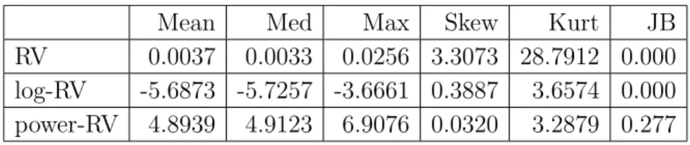
In order to compare the conditional heteroskedasticities, in Figure 1 we plot the squared residuals (ˆε2it), obtained from the AR(1) regressions for RV, log-RV and power-RV, respectively, against each corresponding explanatory variable (lagged RV, log-RV and power-RV). For ease of comparison, superimposed are smooth curves fitted using the LOESS method. It is clear that while the loga-rithmic transformation reduces the conditional heteroskedasticity there is still evidence of conditional heteroskedasticity in the residuals. The power trans-formation further reduces the conditional heteroskedasticity of RV. While the logarithmic transformation reduces the impact of large observations (extreme deviations from the mean), the second plot of Figure 1 suggests that it is not as effective as anticipated. In contrast, the power transformation with a negative power parameter is able to reduce the impact of large observations further. Thus, the results indicate that there is room for further improvements over the logarithmic transformation. A more detailed analysis of the S&P 500 data is provided in Section 6.
3The power parameter is -0.2780 which is the estimate ofλin the proposed model obtained
0.000 0.010 0.020 0e+00 1e−04 2e−04 3e−04 4e−04 Lagged RV Residual Squares −7.0 −6.0 −5.0 −4.0 0.0 0.5 1.0 1.5 2.0 2.5 3.0 Lagged Log−RV Residual Squares 3 4 5 6 7 0.0 0.5 1.0 1.5 2.0 2.5 3.0 Lagged Power−RV Residual Squares
Figure 1. Plots of the squared residuals, obtained from the
AR(1) regressions for RV, log-RV and power-RV, respectively, against each corresponding lagged explanatory variable. Super-imposed are smooth curves fitted using the LOESS method.
2.3. The Nonnegative Semiparametric Model–NonNeg. In this paper,
of Model (2.5),
(2.8) h(RVt, λ) = α+βh(RVt−1, λ) +εt, t = 2, ..., T
where{εt}is a sequence of independentN(0, σε2) distributed random variables
and h(x, λ) is given by (2.6). Ifλ 6= 0, we may rewrite (2.8) as
(2.9) RVtλ = (λα+ 1) +β(RVtλ−1−1) +λεt,
where RVλ
t is a simple power transformation. A special case of (2.9) is the
linear Gaussian AR(1) model when λ= 1:
(2.10) RVt= (α+ 1) +β(RVt−1 −1) +εt.
Ifλ = 0 in (2.8), we have the log-linear Gaussian AR(1) model previously used in the literature:
(2.11) lnRVt=α+βlnRVt−1+εt.
While the specification in (2.8) is more general than the log-linear Gaussian AR(1) model (2.11), it has two potential drawbacks. First, in general, the right hand side of (2.9) has to be nonnegative with probability 1. This re-quirement is violated since a normal error distribution has a support covering the entire real line. Second, the model imposes a simple AR(1) structure for the transformed RV. While an AR(1) structure typically is the most important component in capturing the volatility dynamics, the actual dynamic proper-ties of volatility can be more complicated. See Chernov, Gallant, Ghysels & Tauchen (2003) and ABDL (2003) for evidence against the simple AR(1) struc-ture. In ABDL (2003) the AR(1) specification is augmented with a fractional integrated component to induce long memory in the logarithmic daily RV.
These two drawbacks motivates us to explore an alternative model specifi-cation for RV. Our nonnegative (NonNeg) model is of the form
(2.12) RVtλ =φRVtλ−1+Vt, t= 2, ..., T
where λ 6= 0, φ > 0 and the initial value RV1 is positive with probability 1.
{Vt}is assumed to be a sequence ofm-dependent, identically distributed,
con-tinuous random variables with nonnegative support [γ,∞), for some unknown γ ≥ 0. It is assumed that m ∈ N is finite and potentially unknown. Hence, the specifics of the dependency structure of Vt is left unspecified. So is the
distribution of Vt.
The nonnegative restriction on the support of the error distribution ensures the positivity of RVλ
t . Hence, our model does not suffer from the truncation
problem in the classical Box-Cox model (2.8). When Vt is serially dependent,
the dynamics ofRVtλ are more complex than the dynamics of an AR(1) model. As the distribution of Vt is left unspecified, some very flexible tail behavior
is allowed for. Consequently, both drawbacks in the classical Box-Cox model (2.8) are addressed in the NonNeg model.
One role that the transformation parameter, λ, plays in our model is to sta-bilize the variance, i.e. to induce homoskedasticity (cf. Figure 1). An intercept in the model is superfluous because γ can be strictly positive.
Ifm= 0, our model echoes Equation (2.8) where the normal distribution in (2.8) is replaced with a nonnegative error distribution. If, in addition, λ= 1, our model becomes the discrete time version of Equation (2) in Barndorff-Nielsen & Shephard (2001).
In general, neither the dependency structure nor the distributional form is assumed to be known for the error component. Hence, the NonNeg model combines a parametric component for the persistence with a nonparametric
component for the error. On the one hand, the new model is highly parsimo-nious. In particular, there are only two parameters that have to be estimated for the purpose of volatility forecasting, namely φ and λ. On the other hand, the specification is sufficiently flexible for modeling the error. For example, Vt is not required to have finite higher order moments and can hence
eas-ily incorporate jumps. The specification also allows for a more acute “peak” around the mean. Typically, an additive or multiplicative MA(m) structure may be assumed forVt, the purpose of which is to capture any remaining serial
dependence left uncaptured by the autoregressive component.
As mentioned earlier, there exists a lower bound for the percentage change in volatility in Model (2.2). A similar bound applies to our model. It is easy to show that RVt/RVt−1 ≤ φ1/λ if λ < 0 (upper bound), and RVt/RVt−1 ≥ φ1/λ
if λ > 0 (lower bound). Typical estimated values of φ and λ in (2.12) for our empirical study are 0.639 and -0.278, respectively, implying that RVt cannot
increase by more than 500% from one time period to the next. As we will see later, our proposed estimator for λ depends on the ratios of successive RV’s and hence the bound is endogenously determined.
3. Robust Estimation & Forecasting
3.1. Estimation of φ. For the exceptional situation when λ is known, we
propose to estimate φ using the extreme value estimator (EVE) defined by
(3.1) φˆ= min RVλ t RVλ t−1 T t=2 .
This estimator is the maximum likelihood estimator (MLE) of φ when the errors in (2.12) are independent exponentially distributed random variables Nielsen & Shephard (2003). Interestingly, the EVE is strongly consistent for more general error specifications under a set of mild conditions Preve (2008).
It is robust in the sense that the conditions allow for certain model misspeci-fications in Vt. For example, the order of m-dependence in the errors and the
conditional distribution of RVt may be incorrectly specified. Moreover, the
EVE is strongly consistent even under quite general forms of heteroskedastic-ity. For a more detailed account of the EVE, see Preve (2008).
Like the well known ordinary least squares (OLS) estimator, the EVE is distribution-free in the sense that its consistency does not rely on a particular distributional assumption for the error component. However, the EVE is in many ways superior to the OLS estimator. For example, its rate of convergence can be faster than Op(T−1/2) even when φ < 1, whereas the OLS estimator
converges faster thanOp(T−1/2) only whenφ≥1 Phillips (1987). Furthermore,
unlike the OLS estimator the consistency conditions of the EVE do not involve the existence of any higher order moments.
Under additional technical conditions, Davis & McCormick (1989) and Fei-gin & Resnick (1992) obtain the limiting distribution of a linear programming estimator (LPE) for which the EVE in (3.1) appear as a special case when λ = 1 and the errors are iid (i.e. 0-dependent). The authors show that the accuracy of the LPE depends on the index of regular variation at zero (or infin-ity) of the error distribution function. For example, for standard exponential errors, the index of regular variation at zero is 1 and the LPE/EVE converges to φ at the rate of Op(T−1). In general, a difficulty in the application of the
limiting distribution is that the index of regular variation at zero appears both in a normalizing constant and in the limit. Datta & McCormick (1995) avoid this difficulty by establishing the asymptotic validity of a bootstrap scheme based on the LPE.
It is readily verified that the EVE is positively biased and nonincreasing in T, that is, φ < φˆT2 ≤ φˆT1 with probability 1 for any T1 < T2.4 Hence, the
accuracy of the EVE either remains the same or improves as the sample size increases (cf. Figure 2).
To understand the robustness of the EVE, consider the covariance stationary AR(1) model
RVt=φRVt−1+Vt, t = 0,±1,±2, ...
under the possible model misspecification Vt=Zt+
m
X
i=1
θiZt−i,
where {Zt} is a sequence of non-zero mean iid random variables. For m > 0
the identically distributed errors Vt are serially correlated. In this setting the
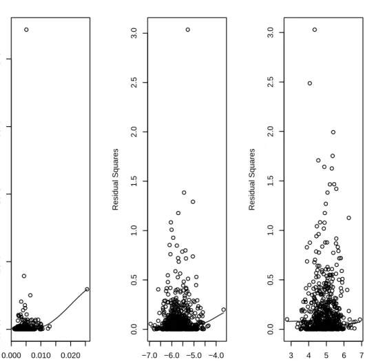
OLS estimator of φ is inconsistent while the EVE remains consistent. In the first panel of Figure 2 we plot 100 observations simulated from the nonnegative ARMA(1,1) model, RVt = φRVt−1 +Zt+θZt−1 with φ = 0.5, θ = 0.75 and
standard exponential noise. In the second panel of Figure 2 we plot the paths of the recursive EVEs and the recursive OLS estimates for φ obtained from the simulated data. In each pass, a new observation is added to the sample. It can be seen that the EVEs quickly approach the true value of φ, whereas the OLS estimates do not. Additionally, the OLS estimates fluctuate much more than the EVEs when the sample size is small, suggesting that in small samples the EVE is less sensitive to extreme deviations from the mean than the OLS estimator.
We now list the conditions under which the consistency of the EVE holds. The proof of the proposition is found in Preve (2008).
1 25 50 75 100 0 5 10 t 1 3 25 50 75 100 0 0.5 0.743 1 T
Figure 2. The top panel displays a time series plot of data
simulated from the nonnegative ARMA(1,1) process RVt =
φRVt−1 +Zt+θZt−1 with φ = 0.5, θ = 0.75 and iid standard
exponential noise. The bottom panel displays the paths of re-cursive EVEs and OLS estimates forφin the misspecified AR(1) modelRVt=φRVt−1+Zt, obtained from{RV1, ..., RVT}, where
T ∈ {3, ...,100}. The solid line represents the EVEs and the dash-dotted line represents the OLS estimates.
Condition 1. In Model (2.12), λ 6= 0, φ > 0 and the initial value RV1 is
al-most surely positive;{Vt}is a sequence ofm-dependent, identically distributed,
nonnegative continuous random variables.
Condition 2. The error component in Model (2.12) satisfies
P(c1 < Vt< c2)<1,
It is important to point out that Condition 2 is satisfied for any error dis-tribution with unbounded nonnegative support.
Proposition 3.1. Denote the EVE in (3.1) by φˆT. Under conditions 1 and
2, φˆT a.s.
−→φ as T → ∞.
3.2. Estimation of φ and λ. In practice, we do not know the true value of
λ. In this section we propose an EVE based two-stage estimation method for λandφ in Model (2.12). The estimators are easily computable using standard computational software such as Matlab. In doing so, we also establish an ex-pression for its one-step-ahead forecast. We then investigate the finite sample performance of the proposed estimation method via Monte Carlo simulations. Estimation of λ and φ is non-trivial, even under certain parametric and simplifying assumptions about Vt. For example, if {Vt} is a sequence of
inde-pendent exponentially distributed random variables it can be shown that the MLEs of λ and φ are inconsistent.5
In our EVE based two-stage estimation method, we first choose ˆλ to mini-mize the sum of squared one-step-ahead prediction errors
ˆ λT = arg min λ∈Λ T X t=2 RVt−RVdt(λ) 2 , where d RVt(λ) = 1 T −1 T X s=2 h ˆ φ(λ)RVtλ−1+Vbs(λ) i1/λ , ˆ φ(λ) = min RVt RVt−1 λT t=2 and Vbs(λ) =RVsλ−φ(λ)RVˆ λ s−1,
5This result also applies to the standard nonlinear least squares (NLS) estimator that
minimizesP
t(RV λ
t −φRVtλ−1)2. In this case the resulting estimator ofλandφis always 0
respectively. The intuition behind the proposed estimation method is that we expect RVdt ˆλT
to be close E(RVt | RVt−1) as T is large. This is not
surprising since Model (2.12) implies that RVt= φRVtλ−1+Vt 1/λ , and E(RVt|RVt−1) =E φRVtλ−1+Vt 1/λ |RVt−1 . In the second stage, we use the EVE to estimate φ,
ˆ φT = ˆφ λˆT = min RVt RVt−1 λˆTT t=2 .
While we minimize the sum of squared one-step-ahead prediction errors when estimating λ, other criteria, such as minimizing the sum of absolute one-step-ahead prediction errors, can be used. We have experimented with absolute prediction errors using the S&P500 data and found that our out-of-sample forecasting results for the NonNeg model are quite insensitive to the choice of the objective function in the estimation stage. However, the objective function with squared prediction errors performs better in simulations. It is important to use the EVE estimator for φ due to its robustness property with respect to serial dependence in Vt.
With an estimated λ and φ, the proposed one-step-ahead semiparametric forecast expression for the NonNeg model is
d RVT+1= 1 T −1 T X s=2 ˆ φTRV ˆ λT T +Vbs 1/ˆλT , whereVbs=RV ˆ λT s −φˆTRV ˆ λT
s−1 is the residual at time periods. Of course, in line
with Granger & Newbold (1976), several forecasts of RVT+1 may be
consid-ered. For example, one could base a forecast on the well known approximation E[h(Y)]≈h[E(Y)] using h(y) = y1/λ. However, this approximation does not
take into account the nonlinearity of h(y). For instance, if Y ∼ N(0, σ2) and h(y) = y2 then E[h(Y)] =σ2 6=h[E(Y)] = 0.
3.3. Monte Carlo Evidence. In the special case of a nonnegative AR(1)
model with iid exponential errors, the distribution of the EVE estimator for φ is nonstandard and asymptotically exponential Nielsen & Shephard (2003). Since our estimator is EVE-based, its asymptotic distribution is likely to be nonstandard and difficult to obtain. Instead of establishing the limiting dis-tribution of the proposed estimators forλand φ, we examine the performance of our estimation method via simulations.
We designed two experiments in which data are generated by the nonnega-tive model
RVtλ =φRVtλ−1 +Zt+θZt−1, t= 2, ..., T
with iid standard exponential driving noiseZt. The parametersλ and φ were
estimated using the proposed two-step method of Section 3.2.
In the first Monte Carlo experiment the true values were set to λ=−0.45, φ = 0.58 and θ = 0.05. In the second experiment the true parameter values are λ = −0.28, φ = 0.64 and θ = 0.15. The values chosen for λ and φ in the experiments are empirically realistic (cf. the results of Section 6). We consider sample sizes ofT = 200,400 and 800. The sample size of 400 is close to the smallest sample size used for estimation in our empirical study, while the sample size of 800 is close to the largest sample size in the study.
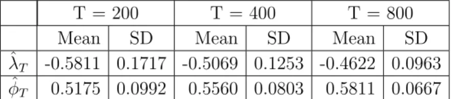
Simulation results based on 5000 Monte Carlo replications are reported in Tables 2 and 3. Several interesting results emerge from the tables. First, the smaller the value of T the greater the sample bias of ˆλT, and ˆφT. Second,
as T increases the bias and standard error of ˆλT, and ˆφT, decreases. It may
Table 2. Simulation results for the proposed two-step
estima-tion method. Summary statistics for ˆλT and ˆφT based on data
generated by the nonnegative process RVλ
t = φRVtλ−1 +Zt +
0.05Zt−1 with iid standard exponential noise. True values for
λ and φ are -0.45 and 0.58. Mean and SD denotes the sample mean and standard deviation, respectively. Results based on 5000 Monte Carlo replications.
T = 200 T = 400 T = 800
Mean SD Mean SD Mean SD
ˆ
λT -0.5811 0.1717 -0.5069 0.1253 -0.4622 0.0963
ˆ
φT 0.5175 0.0992 0.5560 0.0803 0.5811 0.0667
Table 3. Simulation results for the proposed two-step
estima-tion method. Summary statistics for ˆλT and ˆφT based on data
generated by the nonnegative process RVλ
t = φRVtλ−1 +Zt +
0.15Zt−1 with iid standard exponential noise. True values for
λ and φ are -0.28 and 0.64. Mean and SD denotes the sample mean and standard deviation, respectively. Results based on 5000 Monte Carlo replications.
T = 200 T = 400 T = 800
Mean SD Mean SD Mean SD
ˆ
λT -0.3660 0.1099 -0.3113 0.0793 -0.2776 0.0604
ˆ
φT 0.5824 0.0925 0.6242 0.0742 0.6524 0.0610
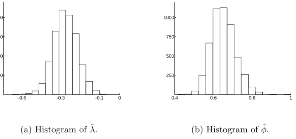
is estimated by ˆλT. Figure 3 plots histograms of ˆλT and ˆφT obtained from
5000 Monte Carlo replications with common sample size T = 800. In sum, it seems that the proposed estimation method works well, especially when T is reasonably large.
-0.5 -0.3 -0.1 0 250 500 750 1000 (a) Histogram of ˆλ. 0.4 0.6 0.8 1 250 500 750 1000 (b) Histogram of ˆφ.
Figure 3. Histograms of ˆλT and ˆφT based on data generated by
the nonnegative processRVtλ =φRVtλ−1+Zt+ 0.15Zt−1 with iid
standard exponential noise. Results based on 5000 Monte Carlo replications with common sample size T = 800. True values for λ and φ are -0.28 and 0.64, respectively.
4. Competing Models
Numerous models and methods have been applied to forecast stock market volatility. For example, ARCH-type models are popular in academic publica-tions and RiskMetrics is widely used in practice. Both methods use returns to forecast volatility at the same frequency. However, since the squared return is a noisy estimator of volatility ABDL (2003) instead consider RV and present strong evidence to support time series models based directly on RV in terms of forecast accuracy. Motivated by their empirical findings, we compare the forecast accuracy of the proposed model against three time series methods, all based on RV: (1) the linear Gaussian AR model (LinGau); (2) the log-linear Gaussian AR model (LogGau) and (3) the logarithmic autoregressive frac-tionally integrated moving average (ARFIMA) model. We also compare the
performance of our model against the exponential smoothing method, a RV version of RiskMetrics. The LinGau and LogGau models are defined by equa-tions (2.10) and (2.11), respectively. We now review the exponential smoothing method and the ARFIMA model.
Exponential Smoothing-ES. Exponential smoothing is a simple method of
forecasting, where the one-step-ahead forecast of RV is given by
(4.1) RVdT+1 = (1−α)RVT +αRVdT = (1−α) T−1 X i=0 αiRVT−i, with 0< α <1.
The exponential smoothing formula can be understood as the RV version of RiskMetrics, where the squared return, XT2, is replaced by RVT. Under
the assumption of conditional normality of the return distribution, XT2 is an unbiased estimator of σ2t. RiskMetrics recommends α = 0.94 for daily data and α= 0.97 for monthly data.
To see why the squared return is a noisy estimator of volatility even under the assumption of conditional normality of the return distribution, suppose that Xt follows Equation (2.3). Conditional on σt, it is easy to show that
Lopez (2001) (4.2) P Xt2 ∈ 1 2σ 2 t, 3 2σ 2 t = 0.2588.
This implies that with a probability close to 0.74 the squared return is at least 50% greater, or at most 50% smaller, than the true volatility. Not surprisingly, Andersen & Bollerslev (1998) find that RiskMetrics is dominated by models based directly on RV. For this reason, we do not use RiskMetrics directly. Instead, we use (4.1) withα= 0.97, which assigns a weight of 3% to the most
recently observed RV. We remark that the forecasting results of Section 6 were qualitatively left unchanged when other values for α were used.
ARFIMA(p, d, q). Long range dependence is a well documented stylized fact
for volatility of many financial time series. Fractional integration has pre-viously been used to model the long range dependence in volatility and log-volatility. The autoregressive fractionally integrated moving average (ARFIMA) was considered as a model for logarithmic RV in ABDL (2003) and Deo, Hurvich & Lu (2006), among others. In this paper, we consider two par-simonious ARFIMA models for log-RV, namely, an ARFIMA(0,d,0) and an ARFIMA(1,d,0).
The ARFIMA(p, d,0) model for the log-RV is defined by (1−β1B−...−βpBp)(1−B)d(lnRVt−µ) =εt,
where the parametersµ, β1, ..., βp and the memory parameterdare real valued,
and {εt}is a sequence of independent N(0, σε2) distributed random variables.
Following a suggestion of a referee, we estimate all the parameters of the ARFIMA model using an approximate ML method by minimizing the sum of squared one-step-ahead prediction errors. See Beran (1995), Chung & Baillie (1993) and Doornik & Ooms (2004) for detailed discussions about the method and Monte Carlo evidence supporting the method. Compared to the exact ML of Sowell (1992), there are two advantages in the approximate ML method. First, it does not require d to be less than 0.5. Second, it has smaller finite sample bias. Compared to the semi-parametric methods, it is also more effi-cient.6 The one-step-ahead forecast of an ARFIMA(p, d,0) withp= 0 at time
6We also applied the exact ML method of Sowell (1992) and the exact local Whittle
estimator of Shimotsu & Phillips (2005) in our empirical study and found that the forecasts remained essentially unchanged.
period T is given by d RVT+1 = exp n ˆ µ− T−1 X j=0 ˆ πj(lnRVT−j −µ) +ˆ ˆ σ2 ε 2 o , and for p= 1 by d RVT+1 = exp n ˆ µ+ ˆβ(lnRVT −µ)ˆ + T−1 X j=1 ˆ πj ˆ β(lnRVT−j −µ)ˆ −(lnRVT−j+1−µ)ˆ +σˆ 2 ε 2 o , where ˆ πj = Γ(j−dˆ) Γ(j + 1)Γ(−dˆ), and Γ(·) denotes the gamma function.
5. Forecast Accuracy Measures
It is not obvious which accuracy measure is more appropriate for the eval-uation of the out-of-sample performance of alternative time series methods. Rather than making a single choice, we use four measures to evaluate forecast accuracy, namely, the mean absolute error (MAE), the mean absolute per-centage error (MAPE), the mean square error (MSE), and the mean square percentage error (MSPE). LetRVditdenote the forecast ofRVtfrom modeliat
time periodt and define the accompanying forecast error byeit =RVt−RVdit. The four accuracy measures are defined, respectively, by
MSE = 1 P P X t=1 e2it, MSPE = 100 P P X t=1 eit RVt 2 , MAE = 1 P P X t=1 |eit|, MAPE = 100 P P X t=1 eit RVt . where P is the length of the forecast evaluation period.
An advantage of using MAE instead of MSE is that it has the same scale as the data. The MAPE and the MSPE are scale independent measures. For a comprehensive survey on these and other forecast accuracy measures see Hyndman & Koehler (2006).
When calculating the forecast error, it is implicitly assumed thatRVtis the
true volatility at timet. However, in reality the volatility proxyRVtis different
from the true latent volatility. Several recent papers discuss the implications of using noisy volatility proxies when comparing volatility forecasts under cer-tain loss functions. See, for example, Andersen & Bollerslev (1998), Hansen (2006) and Patton (2007). The impact is found to be particularly large when the squared return is used as a proxy for the true volatility, but diminishes with the approximation error. In this paper, the true (monthly) volatility is approximated by the RV using 22 (daily) squared returns. As a result, the approximation error is expected to be much smaller than in the case of using a single squared return.
6. Empirical Study
Forecasting S&P 500 Monthly Realized Volatility. The data used in
this paper consist of daily closing prices for the S&P 500 index over the period January 2, 1946-December 31, 2004, covering 708 months and 15,054 trading days. We measure the monthly volatility using realized volatility calculated from daily data. Denote the log-closing price on thek’th trading day in month t by p(t, k). Assuming there are Tt trading days in month t, we define the
monthly RV as RVt = v u u t 1 Tt Tt X k=2 p(t, k)−p(t, k−1)2 , t= 1, ...,708
Jan 19460 Jun 1975 Dec 2004 0.01
0.02 0.03
t
Figure 4. S&P 500 monthly realized volatilities, Jan 1946-Dec
2004. The vertical dashed line indicates the end of the initial sample period used for estimation in our first out-of-sample fore-casting exercise.
where 1/Tt serves the purpose of standardization.
In order to compare the out-of-sample predictive accuracy of the competing methods, we split the time series of monthly RV into two subsamples. The first time period is used for the initial estimation. The second period is the hold-back sample used for forecast evaluation. When calculating the forecasts we use a recursive scheme, where the size of the sample used for estimation suc-cessively increases as new forecasts are made. The time series plot of monthly RV for the entire sample is shown in Figure 4, where the vertical dashed line indicates the end of the initial sample period used for estimation in our first forecasting exercise.
Table 4. Summary statistics for the S&P 500 RV data. JB
is the p-value of the Jarque-Bera test under the null hypothesis that the data are from a normal distribution.
Mean Max Skew Kurt JB ρˆ1 ρˆ2 ρˆ3
RV 0.0037 0.0256 3.307 28.791 0.000 0.576 0.477 0.408 log-RV -5.6873 -3.6661 0.389 3.657 0.000 0.683 0.595 0.511
Table 4 shows the mean, maximum, skewness, kurtosis, the p-value of the JB test statistic for normality, and the first three sample autocorrelations of the entire sample for RV and log-RV. For RV, the sample maximum is 0.0256 which occurred in October 1987. The sample kurtosis is 28.791 indicating that the distribution of RV is non-Gaussian. In contrast, log-RV has a much smaller kurtosis (3.657) and is less skewed (0.389). It is for this reason that we include Gaussian time series models for log-RV in the competition. However, a formal test for normality via the JB statistic strongly rejects the null hypothesis of normality of log-RV, suggesting that further improvements over log-linear Gaussian approaches are possible.
Higher order sample autocorrelations are in general slowly decreasing and not statistically negligible, indicating that RV and log-RV are predictable. To test for possible unit roots, augmented Dickey-Fuller (ADF) test statistics were calculated. The ADF statistic for the sample from 1946 to 2004 is -5.69 for RV and -5.43 for log-RV, which is smaller than -2.57, the critical value at the 10% significance level. Hence, we reject the null hypothesis that RV or log-RV has a unit root.
Forecasting Results. Each competing model was fitted to the in-sample
a forecast frequency of one month is sufficiently important in practical ap-plications, we focus on one-period-ahead forecasts in this paper. However, multi-period-ahead forecasts can be obtained in a similar manner.
We perform two out-of-sample forecasting exercises. In both exercises, we use the recursive scheme, where the size of the sample used to estimate the competing models grows as we make forecasts for successive observations. More precisely, in the first exercise, we first estimate all the competing mod-els with data from the period January 1946-June 1975 and use the estimated models to forecast the RV of July 1975. We then estimate all models with data from January 1946-July 1975 and use the model estimates to forecast the RV of August 1975. This process is repeated until, finally, we estimate the models with data from January 1946-November 2004. The final model estimates are used to forecast the RV of December 2004, the last observation in the sample.
Sample including the 1987 Crash. In the first exercise, the first month for
which an out-of-sample volatility forecast is obtained is July 1975. In total 354 monthly volatilities are forecasted, including the volatility of October 1987 when the stock market crashed and the RV is 0.0256.
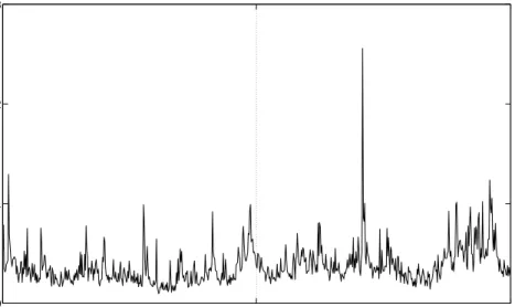
In Figure 5, we plot the monthly RV and the corresponding one-month-ahead NonNeg forecasts for the out-of-sample period, July 1975 to December 2004. It seems that the NonNeg model captures the overall movements in RV reasonably well. The numerical computation of the 354 forecasts is fast and takes less than ten minutes on a standard desktop computer.
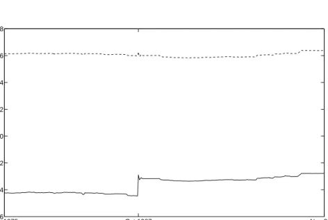
In Figure 6, we plot the recursive estimates, ˆφT and ˆλT. While ˆλT takes
val-ues from -0.45 to -0.28, ˆφT ranges between 0.58 and 0.64. It may be surprising
1980 1985 1990 1995 2000 0 0.01 0.02 0.03 Year
Figure 5. Realized volatility and out-of-sample NonNeg
fore-casts for the period Jul 1975-Dec 2004. Dashed line: S&P 500 monthly realized volatility. Solid line: one-step-ahead NonNeg forecasts.
the transformation parameter, λ, are varying over time. Our empirical esti-mates of λ seem to corroborate well with the optimal value of λ obtained by Goncalves & Meddahi (2006) using simulations in the context of a GARCH diffusion and a two factor SV model. While ˆφT is quite stable, ˆλT jumps in
October 1987.
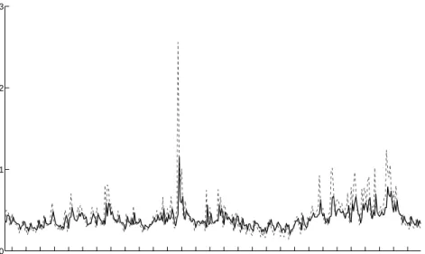
In Figure 7, we plot the NonNeg residuals, Vbt, for the entire sample. Also depicted is a histogram of the residuals. From the histogram, it can be seen that there is no evidence of outliers in Vbt and that there is an acute “peak”
about the mean. These two features suggest that the error term in the NonNeg model tends to take a value around the mean and may explain why the NonNeg model can under-predict (cf. Figure 5).
Jun 1975 Oct 1987 Nov 2004 −0.6 −0.4 −0.2 0 0.2 0.4 0.6 0.8 T
Figure 6. NonNeg recursive parameter estimates for the first
out-of-sample forecasting experiment. Solid line: path of ˆλT.
Dashed line: path of ˆφT.
100 300 500 700 0 0.5 1.5 2.5 3.5 t
(a) Time series plot ofVbt.
0 1 2 3 0 50 100 150 200 (b) Histogram ofVbt.
Figure 7. Time series plot and histogram of the residuals Vbt, obtained when estimating the NonNeg model using the entire sample.
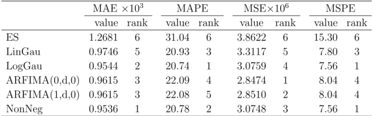
Table 5 reports the forecasting performance of the competing models under the four forecast accuracy measures of Section 5. Several results emerge from the table. First, the relative performances of the competing models are sen-sitive to the measures. Under the MSE measure, the two ARFIMA models ranks as the best, followed by the NonNeg model and the log-Gaussian model. ABDL (2003) found that their ARFIMA models perform well in terms of R2
in the Mincer-Zarnomitz regression. Since the MSE is closely related to the R2 in the Mincer-Zarnomitz regression, our results reinforce their findings. However, the rankings obtained under MSE are very different from those ob-tained under the other three accuracy measures. The MAE and the MSPE ranks the NonNeg model the first while the MAPE and the MSPE ranks the log-Gaussian model the first. Second, the performances of the two ARFIMA models are very similar under all measures. To understand why, we plotted the sample autocorrelation functions of the ARFIMA(0,d,0) residuals for the entire sample and found that fractional differencing alone successfully removes the serial dependence in log-RV. Third, the improvement of ARFIMA(0,d,0) over NonNeg is 7.40% in terms of MSE. On the other hand, the improvement of NonNeg over ARFIMA(0,d,0) is 0.83%, 6.30% and 6.35% in terms of MAE, MAPE, and MSPE, respectively. These improvements are striking as we ex-pect ARFIMA models to be hard to beat. Fourth, ES performs the worst in all cases.
Sample Post the 1987 Crash. To examine the sensitivity of our results with
respect to the 1987 crash and the 1997 crash due to the Asian financial crisis, we redo the forecasting exercise so that the first month for which an out-of-sample volatility forecast is obtained is January 1988 and the last month is September 1997.
Table 5. Forecasting performance of the competing methods
under four different accuracy measures. Results based on 354 one-step-ahead forecasts for the periodJul 1975-Dec 2004.
MAE ×103 MAPE MSE×106 MSPE
value rank value rank value rank value rank
ES 1.2681 6 31.04 6 3.8622 6 15.30 6 LinGau 0.9746 5 20.93 3 3.3117 5 7.80 3 LogGau 0.9544 2 20.74 1 3.0759 4 7.56 1 ARFIMA(0,d,0) 0.9615 3 22.09 4 2.8474 1 8.04 4 ARFIMA(1,d,0) 0.9615 3 22.08 5 2.8510 2 8.04 4 NonNeg 0.9536 1 20.78 2 3.0748 3 7.56 1
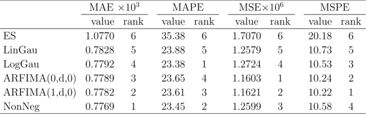
In Figure 8, we plot the monthly RV and the corresponding one-month-ahead NonNeg forecasts for the out-of-sample period, January 1988-September 1997. As before, forecasts from the NonNeg model captures the overall move-ments in RV reasonably well. Table 6 reports the forecasting performance of the competing models under the four forecast accuracy measures. Since the RVs are smaller in this subsample, as expected, the MAE and the MSE are smaller than before. However, the relative performances of the compet-ing models obtained from the subsample are very similar to those obtained from the entire sample. For example, as before the NonNeg model performs the best according to the MAE. Moreover, the two ARFIMA models perform better than the other competing models in terms of MSE.
7. Concluding Remarks & Future Research
In this paper, a simple time series model is introduced to model and forecast RV. The new model combines a nonnegative valued process for the error term with the flexibility of a Box-Cox like power transformation. The transforma-tion is used to induce homoskedasticity while the nonnegative support of the
1989 1991 1993 1995 1997 0 0.002 0.004 0.006 0.008 0.010 Year
Figure 8. Realized volatility and out-of-sample NonNeg
fore-casts for the period Jan 1988-Sep 1997. Dashed line: S&P 500 monthly realized volatility. Solid line: one-month-ahead Non-Neg forecasts.
Table 6. Forecasting performance of the competing methods
under four different accuracy measures. Results based on 117 one-step-ahead forecasts for the periodJan 1988-Sep 1997.
MAE ×103 MAPE MSE×106 MSPE value rank value rank value rank value rank
ES 1.0770 6 35.38 6 1.7070 6 20.18 6 LinGau 0.7828 5 23.88 5 1.2579 5 10.73 5 LogGau 0.7792 4 23.38 1 1.2724 4 10.53 3 ARFIMA(0,d,0) 0.7789 3 23.65 4 1.1603 1 10.24 2 ARFIMA(1,d,0) 0.7782 2 23.61 3 1.1621 2 10.22 1 NonNeg 0.7769 1 23.45 2 1.2599 3 10.58 4
error distribution overcomes the truncation problem in the classical Box-Cox setup. The model is semiparametric as only the support and not the functional form of the error distribution is assumed to be known. Also, the dependency structure of the error process is left unspecified which allows for departures from the dynamics of a conditional AR(1) model. Consequently, the proposed model is highly parsimonious, containing only two parameters that have to be estimated for the purpose of forecasting. A two-stage estimation method is proposed to estimate the parameters of the new model. Simulation studies validate the new estimation method and suggest that it works reasonably well in finite samples.
We empirically examine the forecast performance of the proposed model rel-ative to a number of existing methods, using monthly S&P 500 RV data. The out-of-sample performances were evaluated under four different forecast accu-racy measures (MAE, MAPE, MSE and MSPE). We found strong empirical evidence that our nonnegative model produce highly competitive forecasts.
Why does the simple nonnegative model produce such competitive fore-casts? Firstly, as shown in Section 2.2, the logarithmic transformation may not induce homoskedasticity and normality as well as anticipated. A more general transformation may be needed. Secondly, the nonnegative model is highly parsimonious. Thirdly, we allow for the dependence in the error term to be of an unknown form. This new approach is in sharp contrast to the tra-ditional approach which aims to find a model that removes all the dynamics in the original data. When the dynamics are complex, a model with a rich parametrization is called for. This approach may come with the cost of over-fitting and hence may not necessarily lead to superior forecasts. By combining
a parametric component for the persistence and a nonparametric error compo-nent with unknown dependency structure, our approach presents an effective utilization of more recent and less recent information.
Although we only examine the performance of the proposed model for pre-dicting S&P 500 realized volatility one month ahead, the technique itself is quite general and can be applied in many other contexts. First, the method requires no modification when applied to intra-day data to forecast daily RV. In this context, it would be interesting to compare our method with the pre-ferred method in ABDL (2003). Second, our model can easily be extended into a multivariate context by constructing a nonnegative vector autoregres-sive model. Third, while we focus on stock market volatility in this paper, other financial assets and financial volatility from other financial markets can be treated in the same fashion. Fourth, as two alterative nonnegative models, it would be interesting to compare the performance of our model with that of Cipollino et al. (2006). Finally, it would be interesting to examine the useful-ness of the proposed model for multi-step-ahead forecasting. These extensions will be considered in later work.
Acknowledgments
The authors gratefully acknowledge research support from the Jan Wallan-der and Tom Hedelius Research Foundation unWallan-der Grant No. P2006-0166:1 and from the Singapore Ministry of Education AcRF Tier 2 Fund under Grant No. T206B4301-RS. We wish to thank the editor, an associate editor, three referees, Torben Andersen, Federico Bandi, Frank Diebold, Marcelo Medeiros, Bent Nielsen, and Neil Shephard for very helpful comments. The OX language of J. A. Doornik and ARFIMA package of Doornik & Ooms (2004) were used
to estimate the two ARFIMA models. Matlab code and data used in this paper is available from http://www.mysmu.edu/faculty/yujun/research.html.
References
Andersen, T. & Bollerslev, T. (1998). Answering the skeptics: Yes, standard volatility models do provide accurate forecasts,International Economic Review39: 885–905. Andersen, T., Bollerslev, T., Diebold, F. & Labys, P. (2001). The distribution of realized
exchange rate volatility,Journal of the American Statistical Association96: 42–55. Andersen, T., Bollerslev, T., Diebold, F. & Labys, P. (2003). Modeling and forecasting
realized volatility,Econometrica71: 579–625.
Barndorff-Nielsen, O. E. & Shephard, N. (2001). Non-gaussian ornstein-uhlenbeck-based models and some of their uses in financial economics,Journal of the Royal Statistical Society, Series B63: 167–241.
Barndorff-Nielsen, O. E. & Shephard, N. (2002). Econometric analysis of realized volatility and its use in estimating stochastic volatility models,Journal of the Royal Statistical Society, Series B64: 253–280.
Beran, J. (1995). Maximum likelihood estimation of the differencing parameter for invertible short and long memory autoregressive integrated moving average models, Journal of the Royal Statistical Society, Series B57: 659672.
Bollerslev, T., Chou, R. Y. & Kroner, K. F. (1992). Arch modeling in finance: A review of the theory and empirical evidence,Journal of Econometrics 52: 5–59.
Bollerslev, T., Engle, R. F. & Nelson, D. (1994). Arch models,inR. F. Engle & D. McFadden (eds),Handbook of Econometrics, Vol IV, Vol. 14, Elsevier Science B.V., Amsterdam, pp. 2959–3038.
Box, G. E. P. & Cox, D. R. (1964). An analysis of transformations, Journal of the Royal Statistical Society, Series B26(2): 211–252.
Chen, W. & Deo, R. (2004). Power transformations to induce normality and their applica-tions,Journal of Royal Statistical Society, Series B 66: 117–130.
Chernov, M., Gallant, A. R., Ghysels, E. & Tauchen, G. (2003). Alternative mmdels for stock price dynamics,Journal of Econometrics116: 225–257.
Chung, C. & Baillie, R. (1993). Small sample bias in conditional sum-of-squares estimators of fractionally integrated arma models,Empirical Economics18(4): 791–806.
Cipollino, F., Engle, R. F. & Gallo, G. (2006). Vector multiplicative error models: Repre-sentation and inference,Technical report, NBER.
Datta, S. & McCormick, W. P. (1995). Bootstrap inference for a first-order autoregression with positive innovations, Journal of the American Statistical Association 90: 1289– 1300.
Davis, R. A. & McCormick, W. P. (1989). Estimation for first-order autoregressive pro-cesses with positive or bounded innovations,Stochastic Processes and their Applications
31: 237–250.
Deo, R., Hurvich, C. & Lu, Y. (2006). Forecasting realized volatility using a long-memory stochastic volatility model,Journal of Econometrics 131: 29–58.
Doornik, J. & Ooms, M. (2004). Inference and forecasting for arfima models with an ap-plication to us and uk inflation, Studies in Nonlinear Dynamics and Econometrics
8: 1218–1218.
Duan, J.-C. (1997). Augmented garch(p,q) process and its diffusion limit,Journal of Econo-metrics79(1): 97–127.
Fan, J., Fan, Y. & Jiang, J. (2007). Dynamic integration of time- and state-domain methods for volatility estimation,Journal of the American Statistical Association102: 618–631. Feigin, P. D. & Resnick, S. I. (1992). Estimation for autoregressive processes with positive
innovations,Communications in Statistics - Stochastic Models8(3): 479–498.
Fernandes, M. & Grammig, J. (2006). A family of autoregressive conditional duration mod-els,Journal of Econometrics 127(1): 1–23.
Ghysels, E., Harvey, A. C. & Renault, E. (1996). Stochastic volatility, in C. R. RAO, & G. S. Maddala (eds), Handbook of Statistics, Vol. 14, North-Holland, Amsterdam, pp. 119–191.
Goncalves, S. & Meddahi, N. (2006). Box-cox transforms for realized volatility, Technical report, Department de sciences economiques, Univeriste de Montreal.
Granger, C. W. J. & Newbold, P. (1976). Forecasting transformed series, Journal of the Royal Statistical Society, Series B38: 189–203.
Hansen, P. R. (2006). Consistent ranking of volatility models, Journal of Econometrics
131: 97–12.
Hentschel, L. (1995). All in the family: Nesting symmetric and asymmetric garch models,
Journal of Financial Economics39: 71–104.
Heston, S. L. (1993). A closed-form solution for options with stochastic volatility with applications to bond and currency options,Review of Financial Studies6: 327–343. Higgins, M. L. & Bera, A. (1992). A class of nonlinear arch models,International Economic
Review33: 137–158.
Hyndman, R. J. & Koehler, A. B. (2006). Another look at measures of forecast accuracy,
International Journal of Forecasting22: 679–688.
Jacod, J. (1994). Limit of random measures associated with the increments of a brownian semimartingale,Technical report, Laboratoire de Probabilit´es, Paris.
Lopez, J. A. (2001). Evaluating the predictive accuracy of volatility models, Journal of Forecasting20: 87–109.
Meddahi, N. & Renault, E. (2004). Temporal aggregation of volatility models, Journal of Econometrics119: 355–379.
Morgan, J. P. (1996). Riskmetrics technical document,New York. 4th Ed.
Nielsen, B. & Shephard, N. (2003). Likelihood analysis of a first-order autoregressive model with exponential innovations,Journal of Time Series Analysis24(3): 337–344. Patton, A. (2007). Volatility forecast comparison using imperfect volatility proxies,Technical
report, Oxford University.
Phillips, P. C. B. (1987). Time series regression with a unit root,Econometrica55: 277–301. Poon, S.-H. & Granger, C. W. J. (2003). Forecasting volatility in financial markets: A
review,Journal of Economic Literature41(2): 478–539.
Preve, D. (2008).Essays on Time Series Analysis - With Applications to Financial Econo-metrics, PhD thesis, Uppsala University. Paper II.
Shephard, N. (2005).Stochastic Volatility: Selected Readings, Oxford University Press. Shimotsu, K. & Phillips, P. C. B. (2005). Exact local whittle estimation of fractional
inte-gration,The Annals of Statistics33(4): 1890–1933.
Sowell, F. (1992). Maximum likelihood estimation of stationary univariate fractionally inte-grated time series models,Journal of Econometrics53: 165–188.
Taylor, S. J. (1986).Modeling Financial Time Series, John Wiley and Sons, New York. Yu, J., Yang, Z. & Zhang, X. (2006). A class of nonlinear stochastic volatility models and its
implications for pricing currency options,Computational Statistics and Data Analysis
51: 2218–2231.
Current address: School of Economics, Singapore Management University, 90 Stamford Road, Singapore 178903.
E-mail address: [email protected]
Current address: Department of Information Science/Statistics, University of Uppsala, Box 513 SE-751 20, Sweden.
E-mail address: [email protected]
Current address: School of Economics, Singapore Management University, 90 Stamford Road, Singapore 178903.