I
n f o r m a t i o n
, C
a r e e r
C
o n c e r n s
,
a n d
O
r g a n i z a t i o n a l
P
e r f o r m a n c e
S
t e p h e n
H
a n s e n
Thesis subm itted to the Department of Economics of the London
School of Economics for the degree of Doctor of Philosophy.
UMI Number: U615968
All rights reserved
INFORMATION TO ALL USERS
The quality of this reproduction is dependent upon the quality of the copy submitted.
In the unlikely event that the author did not send a complete manuscript and there are missing pages, these will be noted. Also, if material had to be removed,
a note will indicate the deletion.
Dissertation Publishing
UMI U615968
Published by ProQuest LLC 2014. Copyright in the Dissertation held by the Author. Microform Edition © ProQuest LLC.
All rights reserved. This work is protected against unauthorized copying under Title 17, United States Code.
ProQuest LLC
789 East Eisenhower Parkway P.O. Box 1346
D ecla ra tio n
I certify th a t this thesis is solely my own work other than where I have clearly indicated th at it is the work of others (in which case the extent of any work carried out jointly by me and any other person is clearly identified in it).
The copyright of this thesis rests with the author. Quotation from it is permitted, provided th a t full acknowledgment is made. This thesis may not be reproduced without the prior written consent of the author.
I warrant th a t this authorization does not, to the best of my belief, infringe the rights of any third party.
A b str a c t
This thesis explores how career concerns and information affect organizational perfor mance.
Its first two chapters analyze a principal-agent model in which the agent has career concerns along the lines of Holmstrom (1999) and in which the principal observes the agent’s performance but the agent and the outside labor market do not.
The first chapter shows th at the presence of career concerns with asymmetric infor mation creates a trade-off between turnover and incentives: in order for career concerns to increase, the firm must release talented workers in the future. The chapter applies its theoretical framework to examine the optimal level of labor market competition and firms’ willingness to make general and firm-specific human capital investments.
In the second chapter, the agent works for the principal for two periods, after which labor market competition for talent occurs. W ithin this environment, it explores the firm’s incentives to disclose the agent’s performance to the agent in between the two periods. It finds th at a profit-maximizing disclosure policy (1) always provides some information to workers; (2) never identifies the worst performers; and (3) sometimes does not identify the best performers.
A ck n o w led g m en ts
I would first like to thank my supervisors Gilat Levy and Andrea P rat for their support throughout these past few years. I am extremely lucky to have had them on hand at the start of my academic career. They have not only provided intellectual guidance, but also have known what to say at the right time to keep me focused on the task at hand.
The work in this thesis has benefited greatly from conversations with economists who are too many to name in a page. I would however like to mention Luis Garicano, who listened on numerous occasions to my ideas for chapter two and instilled in me the importance of applied microeconomic theory being applied; Michael Gibbs at the Booth School of Business, who supported and encouraged my work at a critical stage; Oliver Denk, who carefully read drafts of my papers and provided excellent guidance on how to best communicate my ideas; and Michael McMahon, who has not only been a fantastic coauthor, but also a fantastic friend.
I also appreciate the help of two institutions. First, the Bank of England gave me the financial support throughout my PhD th at I needed to attend the LSE. Second, the Kellogg School of Management at Northwestern University kindly hosted me for two quarters at a late stage in my PhD. The facilities there provided an ideal setting for finalizing my research papers.
Of course, completing a PhD requires not only intellectual fortitude, but also emo tional as well. On this dimension, I am grateful to my mother, father, and step-mother, who have always had time to listen; Nathan Foley-Fisher, who has been with me all the way; and Vee Lin Gann, who has been a second mother to me in London.
C o n ten ts
A b s tra c t... 3
Acknowledgments... 4
P reface... 10
1 Turnover and Incentives in Labor M arkets w ith A sym m etric Inform a tion 14 1.1 In tro d u ctio n ... 14
1.2 M o d e l ... 17
1.2.1 Definition of e q u ilib riu m ... 18
1.3 S o lu tio n ... 19
1.3.1 Equilibrium T urnover... 19
1.3.2 Equilibrium Effort ... 22
1.4 A pplications... 23
1.4.1 C om petition... 24
1.4.2 Human capital investments ... 25
1.5 D iscussion... 27
l.A P r o o f s ... 30
l.A .l Proof of Lemma 1 .1 ... 30
l.A .2 Proof of Proposition 1 . 1 ... 30
l.A .3 Proof of Lemma 1 .2 ... 32
l.A .4 Proof of Proposition 1 . 2 ... 32
l.A .5 Proof of Lemma 1 .3 ... 33
l.A .6 Proof of Proposition 1 . 3 ... 33
l.A .7 Proof of Proposition 1 . 4 ... 34
l.A .8 Proof of Proposition 1 . 5 ... 35
2 The B enefits o f Lim ited Feedback in O rganizations 36 2.1 In tro d u ctio n ... 36
2.2 M o d e l ... 42
2.2.2 Motivation for s e t u p ... 45
2.2.3 Definition of eq u ilib riu m ... 46
2.3 Effects of F e e d b a c k ... 47
2.3.1 Second period effort and effort r i s k ... 47
2.3.2 First period effort and coasting incentives ... 50
2.4 Optimal D isclo su re... 52
2.4.1 Optimal contract with high re w ard s... 53
2.4.2 Optimal contract with low r e w a r d s ... 54
2.4.3 Features of Optimal Disclosure P o lic ie s... 56
2.4.4 Robustness ... 56
2.5 Feedback, Competition, and Technology ... 58
2.6 D iscussion... 61
2.A P r o o f s ... 64
2.A.1 Proof of Lemma 2 .1 ... 64
2.A.2 Proof of Proposition 2 . 1 ... 64
2.A.3 Proof of Lemma 2 .2 ... 66
2.A.4 Proof of Lemma 2 .3 ... 66
2.A.5 Proof of Proposition 2 . 2 ... 67
2.A.6 Proof of Lemma 2 .4 ... 69
2.A.7 Proof of Proposition 2 . 4 ... 70
2.A.8 Proof of Proposition 2 . 6 ... 72
2.A.9 Proof of Proposition 2 . 7 ... 74
2.A. 10 Proof of Lemma 2 .6 ... 74
3 A ssessing th e Effectiveness of M ixed C om m ittees: E vidence from th e B ank o f England M PC 75 3.1 In tro d u ctio n ... 75
3.2 Previous Research on MPC V o t i n g ... 77
3.3 MPC B ackground... 78
3.4 Committee Voting M odel... 80
3.4.1 Assumptions and s e t - u p ... 80
3.4.2 Member b e h a v io r... 83
3.4.3 Mixed committees and w elfare... 88
3.5 D a t a ... 90
3.6 Econometric Modelling and R e s u lts ... 96
3.6.1 Probability of D e v ia tin g ... 96
3.7 Alternative M o d e ls ... 105
3.7.1 Career Concerns ... 106
3.7.2 Asymmetric P re fe re n c e s ... 108
3.7.3 Testing both to g e th e r... 110
3.8 A Natural E x p e rim e n t... I l l 3.9 Conclusion... 115
3.A P r o o f s ... 117
3.A.1 Proof of Proposition 3 . 1 ... 117
3.A.2 Proof of Proposition 3 . 2 ... 117
3.A.3 Proof of Proposition 3 . 3 ... 119
3.A.4 Proof of Proposition 3 . 5 ... 120
List o f F igu res
2.1 Example of Rating D is trib u tio n ... 37
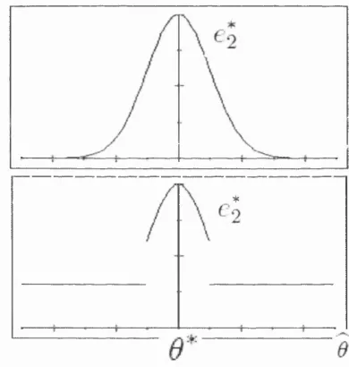
2.2 Equilibrium Effort with Full and Partial D is c lo s u re ... 48
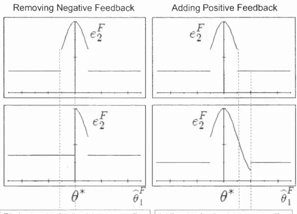
2.3 The Effects of Feedback on First Period E f f o r t... 51
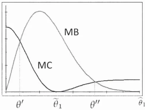
2.4 The Marginal Benefit and Cost of Information D isclosure... 55
3.1 Member Preferences ... 84
3.2 Member Preferences ... 85
3.3 Decision Rules for Members 1 and 2 Given dn and Sn ... 85
3.4 The Effect of Member 1 Disclosure on Member 2 Decision Rule ... 86
3.5 Votes and Decisions of the Monetary Policy C o m m itte e ... 94
L ist o f T ables
2.1 Performance Appraisal Use by In d u stry ... 62
3.1 Distribution of Unique Votes Across M e e tin g s ... 82
3.2 Sample Statistics by Member ... 92
3.3 Total and Percentage Deviations using 3 Different Approaches, by Member 95 3.4 Logit Model - Basic Regression R e s u lts ... 99
3.5 Logit Model - Experience Regression R e s u lts ... 101
3.6 Logit Model - Robustness to Different Experience V ariables... 102
3.7 Level and Vote Variability Regression R e s u l t s ... 104
3.8 Estimates of “Experience-Effect” by Member Type: Career Concerns . . 108
3.9 Estimates of “Experience-Effect” by Member Type: 110 3.10 Estimates of “Experience-Effect” by Member Type: Combined Career Concerns and Asymmetric Preferences R eg ressio n ... I l l 3.11 Estimates of “Experience-Effect” by External Type: Career Concerns Re gression from Natural E xperim ent... 113 3.12 Estimates of “Experience-Effect” by External Type: Combined Career
P refa ce
Ever since Fama (1980) proposed the idea th at a worker’s concern for his reputation could substitute for explicit incentive schemes, economists have recognized the poten tial importance of career concerns in explaining behavior. Today, the career concerns framework laid out in Holmstrom (1999) has become a workhorse model in applied or ganizational economics. One reason is that the prediction from Holmstrom (1979) th a t optimal explicit incentive schemes should depend on every available signal th at is (con ditionally) correlated with output is manifestly not borne out in the real world. Instead, implicit incentives appear more important for explaining why workers exert effort, es pecially in professional service firms, which are playing an increasingly crucial role in modern economies.
While economists have a fairly solid grasp of how career concerns operate at the individual level, what is much less clear is how to design organizations in which career concerns operate. W ith explicit contracting, organizational design is not a first-order problem because the goal is to construct the optimal mapping from output signals to wage payments. In contrast, career concerns depend crucially on institutional details such as the quantity of information available to actors inside and outside organizations and the rewards th at accrue to those perceived as more talented. The central goal of this thesis is to uncover these relationships and to show how organizations can use them to improve overall performance. For the most part, the analysis consists of applied microeconomic theory in its most literal sense. That is, the chapters use game-theoretic models to shed light on real-world phenomena, in many cases generating testable implications. The thesis is therefore a contribution to the growing field of Organizational Economics, which seeks to understand the forces th at shape non-market institutions such as internal labor markets, bureaucracies, committees, and corporate hierarchies.
It is important to point out two main weaknesses in the analysis before summarizing the key results. First, the majority of the conclusions th at the chapters reach depend on particular modelling assumptions, and may not hold in more general environments. General career concerns models are very difficult to solve, so the chapter uses simple functional forms for production technologies, and specifies particular distributions for random variables. Second, although the first two chapters generate testable predictions, the thesis does not provide any empirical analysis to examine them. On the other hand, many of the empirical findings in the third chapter (written jointly with Michael McMa hon) are explored informally, not with an explicit model. All the chapters would benefit from stronger links between theory and data.
principal privately observes an agent’s output within a competitive labor market. This is a natural situation for career concerns to arise, because when outsiders cannot observe output, contracting on it is presumably not possible. The introduction of asymmetric information also adds more richness to the canonical Holmstrom model, in which all participants in the labor market have the same information at all points in time; in particular, it allows one to discuss a range of important human resource management policies about which the Holmstrom model is silent.
In the first chapter, an agent (the worker; he) matches with a principal (the employer; it) for an initial period, after which labor market competition takes place and the employer either retains or releases the worker for a second period. The equilibrium outcome of labor market competition is similar to th at in Waldman’s (1984) well-known paper: the employer retains the worker whenever his expected talent is above a threshold and releases the worker whenever his expected talent is below it. This is inefficient because the employer releases the worker with positive probability even though he always generates more output with the employer than he does with other firms. In the first period, the worker exerts effort because the wage he will be paid if the employer retains him is higher than the wage he will be paid if it releases him. A crucial result is th at whenever second period output is convex in worker talent, this wage difference—and therefore the strength of career concerns—is increasing in the probability th at the agent is released. So, equilibrium turnover is positively correlated with equilibrium effort.
The results suggest th at policies th at jointly affect turnover and effort must resolve a basic trade-off between matching and incentives, and the first chapter presents two applications. The first is to competition policy. Increased labor market competition worsens second period social surplus by increasing turnover, while improving first period social surplus by increasing effort. The same tension also arises when the employer can choose whether to invest in general or firm-specific human capital. Both kinds of human capital inversely affect the ability of the employer to retain talented workers in the second period and its ability to motivate them in the first. The fact th a t the presence of career concerns influences optimal competition and human capital investment means th at traditional analyses of these policy choices may be missing important incentive effects.
First, it creates uncertainty for the worker about his second period effort level, which increases his disutility from joining the employer. Second, when the worker learns his performance, the employer’s belief about his second period effort choice depends on his first period output. So, the worker can use first period effort to influence the amount of effort th at the employer expects him to exert in the second.
The optimal disclosure policy has three notable properties. First, it always involves some, but not full, disclosure. Second, the worker never learns th a t his performance is among the worst possible. Finally, in some situations, the worker does not learn th at his performance is among the best possible. These results are im portant because real world performance appraisals tend not to identify poor performers, and to concentrate ratings in the center of the distribution. Observers often argue th at these patterns reflect some dysfunctionality in appraisal systems, but in fact the rating distributions th at arise from optimal disclosure policies have much in common with real-world distributions. This is not equivalent to saying th at rating systems are always perfect, only th at they may not be as bad as they first appear.
The third chapter (written jointly with Michael McMahon) is quite distinct from the first two. It no longer considers a principal-agent model and no longer explicitly models career concerns. The question it seeks to ask is whether monetary policy committees can benefit from having heterogeneous experts. It is pertinent because some countries (like the UK) appoint people to their monetary policy committees from outside their central banks, while some countries (like the US) do not. To address the issue, it builds a theoretical model to explore the dimensions along which mixed committees might out perform homogeneous ones. The central result is th at if the committee designer knows experts’ beliefs about long-term macroeconomic conditions, it should appoint the expert with the most moderate belief as the sole committee member, and allow all other experts to advise him. The only rationale for having different experts on the same committee is if the committee designer does not observe beliefs. In this case, drawing experts from two different belief distributions can produce a more moderate median voter than drawing experts from only one if every member votes according to his personal view about what is the best policy.
C h ap ter 1
T urnover and In cen tives in Labor
M ark ets w ith A sy m m etric
In form ation
1.1
In tro d u ctio n
There are two important sources of value th at firms enjoy from new workers: their initial productivity and the option value from retaining talented workers in the future. Thus, a firm must achieve two distinct goals to maximize the benefit from employing workers. First, it must provide effort incentives to motivate workers. Second, it must use the information it obtains after observing worker performance to make appropriate retention decisions. Failure to adequately address either issue will impair overall performance.
Of course, there are numerous possible frictions th at may prevent optimal retention and limit effective incentive provision. This chapter focuses on asymmetric information between an employer and an outside labor market as a source of both matching and contracting inefficiencies. In itself, the fact th at asymmetric information distorts labor market outcomes and creates contracting difficulties is not surprising. Instead, the main contribution of this chapter is to show that the ability of firms to retain talented workers under asymmetric information is in many situations negatively related to worker moti vation when effort incentives come from career concerns. In this case, firms’ ability to retain talented workers is inversely related their initial productivity.
uninformed labor market. Asymmetric information implies th a t the 'employer can only pay one wage to retained ability types, and so in equilibrium it releases the worker if his ability falls below a threshold. This is inefficient because every ability type is more productive with the employer than an outside firm in period two.
As explicit contracts can only be written for publicly observable variables, they are not feasible when only the employer observes output. Effort incentives for the worker must therefore arise implicitly, and the chapter assumes they come from career concerns a la Holmstrom (1999). Since career concerns incentives depend on expected future earnings, this choice of contracting instrument creates a tight relationship between the worker’s period one effort and the equilibrium outcome of the bidding game between the employer and outside firms. In the second period, the worker earns higher wages if he is retained by the employer than if he is released, so his second period payoff improves discreetly if the employer’s belief about his ability crosses the retention threshold. He exerts effort in the first period in order to increase the employer’s belief about his talent and increase his future expected payoff—the standard signal jamming logic.
A key assumption in the model is th at second period output is convex in worker tal ent. The implication is th at raising the retention threshold increases the expected market output of retained ability types by more than it increases the expected market output of released ability types. This in turn increases the difference between the equilibrium wage paid to retained and released ability types, which strengthens career concerns. However, raising the retention threshold also increases the probability of turnover. Of course, the retention threshold itself is endogenous. It is primarily determined by two deep parame ters th at measure worker productivity in the market and with the employer, respectively. Increasing either parameter has opposite effects on effort and turnover. When market productivity increases, the retention threshold increases, as does the amount the market is willing to pay every ability type. Both effects increase the wage difference between retained and released ability types, but the former worsens matching. By contrast, when employer productivity increases, the threshold decreases, reducing effort but improving matching. This is the fundamental logic underlying the chapter.
competition th at can lie anywhere from zero to one, depending on the relative magnitudes of the distortions.
The second apphcation of the model examines the employer’s firm-specific and general human capital investment incentives. Increasing general human capital raises the equi librium retention threshold, increasing turnover along with effort. When effort costs are low enough, the firm is willing to invest in general human capital even though it limits its ability to retain talent. Firm-specific human capital presents the opposite trade-off. In creasing it decreases turnover and effort through reducing the retention threshold. Thus, investment in firm-specific skills will not occur when effort is highly sensitive to variations in wages—i.e., when effort costs are low.
The value added of the chapter lies not in analyzing labor market outcomes or career concerns per se, but in tying them together to show that two of the most basic problems facing firms regarding human resource management may not be possible to resolve si multaneously. In fact, the very popularity of adverse selection labor market models and career concerns models highlights the importance of combining both for a clearer picture of how organizations function. Doing so not only reveals an inverse relationship between incentives and turnover, but also uncovers new dimensions on which competition policy and human capital investments might have an impact.
R e la te d L ite r a tu r e The Waldman (1984) model of adverse selection labor market com petition is the closest to the one presented in the chapter, although there are other papers th at examine the consequences of strategic bidding in labor markets with asymmetric in formation (see Greenwald 1986, Bar-Isaac, Jewitt, and Leaver 2008, Li 2008). The crucial assumption is th at bidding occurs sequentially, beginning with the employer and followed by the outside firms. The end of the chapter will discuss how the results depend on this bidding structure.
The career concerns literature th at began with Fama (1980) and Holmstrom (1999), has, for the most part, considered the interactions between one principal and an agent, or among multiple identical principals and an agent. This chapter, in contrast, considers the case in which an agent interacts with multiple principals th at differ both in terms of their productivity and their information about the agent’s output.
to generate effort. Moreover, Schmidt focuses on product market competition, and this chapter on factor market competition.
Acemoglu and Pischke (1998) and Acemoglu and Pischke (1999) argue th at an em ployer will only undertake general human capital investments when it can capture some of the associated gain in worker productivity. Here, the employer does not capture any of the second period surplus from general human capital investment, and yet it still in vests in general skills because by increasing the labor market’s valuation of talent, it strengthens career concerns.
Finally, Mukherjee (2008) combines adverse selection labor market competition with career concerns (and explicit contracting) in order to study an employer’s incentive to disclose information to an outside market. He does not study the relationship between turnover and effort under asymmetric information.
The rest of the chapter proceeds as follows. The next section lays out the model and the subsequent one presents the solution, highlighting how turnover and incentives jointly depend on productivity parameters. The fourth section applies the model to competition and human capital investments, illustrating how they create trade-offs between effort and matching. The final section discusses the assumptions th at underlie the model, and the implications of changing them.
1.2
M od el
In period 1, a worker (he) matches with a firm (it) F. The worker’s first period output is yi = 9 + e where 0 ~ U[ 0,1] is worker talent and e is worker effort. The cost of effort function for the worker is c% (e), where x satisfies the standard properties x ' > 0? x" > 0? lime_>o X (e) — 0 and lim^oo x (e) = oo. The c > 0 parameter is a measure of the cost of effort, and will play an important role in determining how sensitive is equilibrium effort to wage variation. The worker has an outside option equal to 0.
In addition to F t there is an outside labor market th at consists of a large number of firms indexed by j G J . A crucial assumption is th at F perfectly observes yi but th at no firm j does; there is thus asymmetric information. This captures the fact th a t since F works more closely with the worker than does the outside market, it is in a better position to judge the quality of his output.
firm th a t offers him the highest wage. If the maximum wage he is offered by the outside market equals the wage that F offers him, he remains with F; if more than one outside firm offers him the highest wage, he joins each with equal probability; and if his highest wage offer is 0 he takes his outside option. All firms incur an arbitrarily small cost 8 from making wage offers, which could for example reflect the legal costs of drafting a wage contract.
If the worker remains with F for period 2, his output is y.f = f 6 N and if he moves to an outside firm it is = mON, where f > m > 1 and N > 1. The assumption on the magnitudes of the productivity parameters / and m implies th a t every ability type is more productive with F than with an outside firm in the second period. In section 1.4, the chapter gives / and m more specific interpretations, but for now they are left as abstract parameters.
The assumption th at N > 1 implies th at second period production is convex in talent.1,2 While the particular functional form for y2 is not itself crucial for the results of the chapter, convexity is. The exact role it plays will become clear in the next section.
In the model, there is no contracting on output since it is not publicly observable. Instead, all effort incentives will come from career concerns. Thus, the fact th at second period production does not depend on effort is without loss of generality, since career concerns do not exist in the final period of the game.
1 .2 .1
D e fin itio n o f eq u ilib riu m
The chapter uses the Perfect Bayesian Equilibrium concept to solve the model. After observing yi, F forms a belief 0*" on worker talent. Denote by 0 F the set of all possible realizations of 9F , and let wF : 0 F —►W F be F ’s strategy in the bidding game. Let fu7 be market firm f s belief about the strategy th at F employs, and let uft : W F —►WJ be the strategy th at each market firm j employs. Furthermore, let eF and eJ denote the beliefs of firm F and j on worker effort.
The equilibrium set of strategies wF* U {w^*}J-=l and beliefs {wj *}j=1 must satisfy the following conditions:
u?* maximizes E — w* — 1 (w7 ^ 0) £ \/wF given w \ e7, and \u?* (1.1) wF* maximizes E \y2 \ ~ wF ~ 1 ^ 0) 8 given eF and {uP*}^=1 (1.2)
wj * = wF* (1.3)
1The discussion section provides a motivation for this assumption.
Condition (1.1) states th at the strategies employed by market firms constitute a Nash Equilibrium; (1.2) th at F maximizes profit given the behavior of the labor market; and (1.3) th at the belief of each market firm about the strategy employed by F is consistent with its actual strategy.
wF* U {^'*}j=1 implicitly defines an ability-wage schedule w Let ew be the worker’s actual period 1 effort. Equilibrium effort e* must satisfy
ew = arg max —cy (e) + w ^ (1.4)
^ = y i ~ e F (1-5)
e* = ew = eF = e-7 (1-6)
(1.4) requires the worker to maximize utility; (1.5) requires Bayesian learning on the part of the firm; and (1.6) requires every firm’s belief about worker effort to be consistent with the worker’s effort choice.
D efinition 1.1 A Perfect Bayesian Equilibrium of the model satisfies (1.1)-(1.6).
The remainder of the chapter solves the model according to Definition 1.1
1.3
S olu tion
This section derives the implications of the model for turnover and effort and emphasizes their relationship to the / and m parameters. Although the model presented above is relatively simple, it delivers the important insight th at increased effort implies increased turnover. The first part of the section derives properties of the equilibrium bidding strategies and their relationship to turnover, while the second part derives first period equilibrium effort as a function of the equilibrium wage schedule. The section does not impute any welfare implications to the findings, but instead leaves this for the applications presented afterwards.
1.3 .1 E q u ilib riu m T u rn over
Since the labor market bidding game is sequential, the first step involved in solving it is describing the behavior of the outside firms after they observe wF. Condition (1.3) implies th a t all outside firms must share the same belief about F ’s strategy, so th at vP = w. Moreover, condition (1.6) implies th at every outside firm believes th a t &F rsj
Lem m a 1.1 I f wF ^ 0 and E [m9N \ wF, w] — wF — 6 > 0, or if wF = 0 and E [mQN | w F,w ] — 5 > 0, then maXj Wj = E [mON | wF,ui] — 5. Otherwise, = 0 Vy. If F does not pay the worker a wage at least equal to the expected surplus he could generate in the labor market, then one outside firm will pay him a wage equal to the expected surplus. The result follows from Bertrand bidding, which implies th at no outside firm can capture any surplus from the worker.
The behavior of the outside firms influences the bidding behavior of F through setting the worker’s outside option. The next result describes its equilibrium strategy.
P rop osition 1.1 The equilibrium strategy of F satisfies
behavior identified in Lemma 1.1 leads to two wages in equilibrium: one to ability-types th at F retains and one to ability-types th at F releases. The following assumption pins down the latter.
the surplus he creates is positive.
The reason th at F cannot pay any two retained ability-types two different wages is th at wages cannot credibly signal private information. If F paid two different retained types two different wages, and the outside market believed these wage offers credibly communicated private information, F would have an immediate incentive to “lie” to the market and tell it th at the higher ability-type was the lower one since it would save on wage costs. Within the set of retained workers, communication between F and the outside market is impossible.3
3The intuition is similar to that in the cheap talk literature (Crawford and Sobel 1982). Within the set of retained types, the sender of private information (the firm) has no preference concordance at all with the receiver (the outside labor market), so communication is impossible.
(1.7)
where 6* uniquely satisfies
(1.8)
In words, F retains the worker if and only if its belief on his talent exceeds 6* and pays all retained ability-types a wage independent of 6F that is equal to their expected market productivity conditional on 6F C [#*,!]• This strategy combined with the labor market
A ssu m p tio n 1.1 0 < 5 < E m6N+1 \ 6F < 0* = m^ * |1—
The reason released ability-types earn a flat wage is costly bidding. W ithout costly
n /q* \ N + 1
bidding, F could still only retain ability-types above 0* at wage — ; however, it could credibly communicate its private information to the market for ability-types below 9* since providing information would be costless and not affect second period profit. For example, one possible equilibrium strategy for F could satisfy w F* = 6F — e if 0* < e* for some arbitrarily small e. An outside firm would then hire ability-type 0^ whenever m 9F — 5 > 0 at wage m ^ —S. F ’s employing this strategy would lead to a different ability-wage schedule than its employing the strategy specified in Proposition 1.1. This would in turn impact on the worker’s first period effort incentives. Among the different equilibria of the costless bidding game, the most plausible one would maximize profit. However, solving for the optimal amount of information provision to the outside market is not the focus of this chapter. Assuming costly wage offers not only avoids this problem, but also has a realistic interpretation.
A crucial feature of this equilibrium is inefficient matching: since / > m, any turnover is inefficient. However, since (1.8) has a solution that lies within (0,1), F releases the worker with positive probability in equilibrium. The basic reason is wage pooling. F must earn zero profit on the lowest retained ability type while paying him a wage equal to the expected market output of all ability-types above his. Since the output of the lowest ability-types is near 0, F cannot profitably retain them .4
The following result summarizes the effect of the productivity parameters on equilib rium turnover.
Lem m a 1.2 9* is strictly decreasing in f , strictly increasing in m, and bound between 0
and 1.
When / increases, F earns more on every worker type. Since an outside firm’s willingness to bid for the worker is unchanged, this lowers 9* and decreases turnover. When m increases, the outside market is willing to pay more for every ability-type, so F must raise the wage it pays to retained workers. This reduces the number of workers it can profitably retain, increasing 9* and lowering expected second period profit. Moreover, one can also easily show th at lim x ^ ^ 9* = 0, in which case the probability of turnover
771
tends to 0, and th at l i m x - 9* = 1, in which case the probability of turnover tends to 1.
m
1 .3 .2
E q u ilib riu m Effort
To derive first period effort, one needs to look at the entire ability-wage schedule. Com bining the results from above gives
_m_ l-(g*)N+1 qF > N + l 1 - 9 * u — U
_rr^ ( d * ) N+1 jf Q F < Q* N + l 9* 11 V ^ U •
In other words, the worker’s second period earnings are higher if he is retained by F than if he is released. There is thus a reputational reward associated with remaining with F. The size of the reputational reward is given by
W ( T ) = m 1 - ( e *)JV+1 m (6*)n+1 N + l 1 - 0 * N + l 0*
TO 1 - (0*)W
JV + 1 1 - 0 * ' (1.9)
Since contracting on output is not possible, effort incentives for the worker arise solely from the desire to signal a high ability to his employer in order to increase the probability of earning W (9*). The next result establishes the dependence of equilibrium effort on this quantity.
P r o p o s itio n 1.2 Equilibrium effort satisfies
* ' « ■ ) . (1.10)
c
Because 0 is uniformly distributed on [0,1], a marginal increase in effort will increase P r 0F >9*\ by a constant amount 1, the probability density function for a uniform random variable.5 Equilibrium effort equates the marginal benefit of effort—1 x W (9*)— with the marginal cost—cx'-6
Clearly, the size of the reputational reward is key for determining equilibrium effort. As it changes, so too will e* and first period profit for F.
L e m m a 1.3 W (9*) is decreasing in f and increasing in m .
This result hinges on the assumed convexity of second period output in talent. When the retention threshold 9* increases, the newly released types are more talented than
tech n ica lly speaking, this is not true if e is large enough to guarantee that 6F > 6* . In fact, the proof of the result shows that equilibrium effort can never lie at such a corner solution.
the previously released types and less talented than the newly retained types. This means th at the expected output of both retained and released types increases following an increase in turnover. Convexity implies that the expected output of retained types increases by more than the expected output of released types. Hence, the difference in the wage paid to retained and released types increases with turnover. Therefore, an increase in / reduces W (9*) since it decreases 6*, while an increase in m has two complementary effects: it increases W (9*) both through increasing 0* and directly raising the value th a t the outside firm place on any ability-type.
Comparing Lemma 1.3 with Lemma 1.2 leads to the immediate conclusion th at changes in the productivity parameters that decrease turnover reduce first period ef fort and vice versa. To put it another way, the model predicts th a t in a cross-section of firms, after controlling for / (and N), one should observe a positive relationship between turnover and effort, and likewise after controlling for m (and TV).7 This is the central message of the chapter: under asymmetric information, the employer can either motivate the worker in the first period or retain him in the second, but not both.
The results suggest th at policies designed to alter the / and m parameters will have to take into account a trade-off between turnover and effort. The next section explores this idea in more detail. First, though, it is important to discuss how sensitive is effort to changes in / and m in order to determine the relative magnitudes of the associated costs. As one can see from (1.10), e* is more sensitive to differences in W (6*) the smaller is c, the cost of effort parameter. Essentially c measures the importance of career concerns. When it is large, signalling is costly, so that career concerns are weak; when it is small, signalling is cheap, so th a t career concerns play a larger role in the worker’s effort choice.
1.4
A p p lica tio n s
While the results so far are useful for illustrating the inverse correlation between turnover and effort, it is silent about how to interpret the m and / parameters or why they might take on particular values. This section instead models m and / as deliberate policy choices. The first application is to a social planner choosing the optimal level of competition, and the second is to the firm choosing levels of firm-specific and general human capital. In both cases, the optimal policy must balance the trade-off between incentives and matching.
1.4.1
C o m p e titio n
In order to apply the model to competition, one can write m as the following random variable, realized between periods 1 and 2:
{
/ — e with probability p 0 with probability 1 — pwhere e G (0, / ) . If the realization of m is 0, then the worker has no value in the outside market, and F only needs to pay the worker his outside option in order to retain him. If the realization of m is / — £, then F must bid for the worker and pay a positive wage to retain him. p is therefore a natural measure of competition, since it can be interpreted as the probability with which the employer faces another firm in the bidding game. Here, p measures factor market competition, not product market competition, and when p = 0, F is a monopsonist, not necessarily a monopolist. Finally, e measures the output loss when the worker leaves F. Such a loss might arise for many reasons, but the most natural motivation is firm specific human capital, broadly speaking. As e —> 0, then F and the outside firms become identical. Its role in determining the optimal level of competition is discussed below.
A social planner th at can choose the level of competition will select
p* - argmax e* - c% (e*) -f E [;y2}. (1.11)
p
In (1.11), E [2/2] refers to total expected second period output, not just expected second
period output in F. Denote by 6* (e) the retention threshold if m = / — e and W (9*) the wage difference between retained and released workers when m = f — e 8
p* must balance two forces. Whenever m = f —e, the employer inefficiently releases all ability types below 9* (e), leading to an output loss of e (6*(e))N+1. Increasing p increases the probability th at this loss occurs and so damages social welfare. On the other hand, one can write equilibrium effort (from Proposition 1.2) as
x ' ( O = P E E ! , (1-12)
c
meaning th at increasing p increases equilibrium effort. The reason is that, conditional on m = 0, the worker’s second period wage is 0 no m atter what his employer’s belief about his ability, so career concerns do not arise. On the other hand, when m = f — e, there is a reputational reward for signalling an ability above $*, meaning th at career concerns
motivate effort.
A s su m p tio n 1 . 2 W (9*) < 1.
Assumption 1.2 implies th at even when competition is maximal (i.e., p = 1), the worker’s effort is less than first-best. So, increasing p unambiguously increases first period social surplus.
P ro p o s itio n 1.3 A unique p* G [0,1] exists. Moreover, limc-.oop* = 0, limc_>oT* — 1; and ^ < 0 whenever p* G (0,1).
The uniqueness of p* arises from the fact that while the marginal decrease in second period output is constant in p, the marginal increase in first period surplus is decreasing in p since it is concave in effort. The results on the c parameter arise because the welfare gain from moving effort closer to its first-best level is decreasing in the cost of effort. The novel aspect of Proposition 1.3 is th at it derives optimal competition in terms of its impact on the internal and external labor market. The model shows th at the effects of competition go beyond what regulators usually consider, and th at competition can endogenously determine firm productivity.
R e m a rk 1.1 lime_+0 p* = 1
When e —► 0, the employer and the outside firms become identical in the sense th at the worker is equally productive in the second period no m atter where he is employed. The only rationale for limiting competition in the model is to reduce the expected loss in second period output arising from turnover. So, when all firms are identical, the social planner should maximize competition in order to make first period effort as high as possible. The fact th at maximum turnover results does not affect E [2/2] • Loosely
speaking, perfect competition on the intensive margin (eliminating match-specific human capital among potential competitors) implies the social desirability of perfect competition on the extensive margin (ensuring potential competitors actually compete).
1 .4 .2
H u m a n c a p ita l in v e stm e n ts
allows F to choose g and h prior to period 1 but after F and the worker have agreed any period 1 wage payments.9
To simplify the presentation, the section first considers the case in which F can invest in general human capital when firm-specific human capital is fixed at some level h*. W ithout investment, general human capital is g'. However, F can pay a cost K in order to increase g to some g" > g'. To examine investment incentives, one can write the employer’s objective function as
E [ Vl + y2] - l ( g = g " ) K
= \ + ( X T 1 ( ^ ) + [l - ( * T +1] - 1 (ff = 9") K. (1.13)
Investment in general human capital affects profit through increasing the retention thresh old 6*, which increases effort but also increases turnover. As investment in g is costly,
the firm will only ever undertake it if the resulting increase in effort is large enough to both compensate for the investment outlay and the associated reduction in second period profit. Since c measures the sensitivity of effort to changes in 6*, its value determines
whether investment takes place.
P rop osition 1.4 F chooses g = g" if and only i f O < c < c * < o o .
A long-standing argument dating back to Pigou (1912) maintains th a t firms tend to under-invest in general human capital because the resulting productivity gains simply increase the wage payments th at they must pay to retain workers. Since the rate of return on general human capital investment is thus 0, firms will not be willing undertake
them. Ignoring effort for a moment, the situation in this model is even worse. F not only fails to increase the rents it earns on retained workers after investing in their general productivity, it actually reduces the number of ability-types it can retain. Thus, from the perspective of period 2, the rate of return on investment in g is actually negative.
While much of the human capital literature ignores incentive issues, the model demon strates th at the effect of general skills on effort is just as im portant a determinant for investment as their direct effect on future productivity. W ith career concerns, the value th at the labor market places on workers drives their effort choices. By increasing its employee’s general human capital, F increases the amount th at outside firms are willing to pay for talent, increasing W (6*). Proposition 1.4 suggests th a t empirical estimates
of the returns to general human capital investment may be underestimating their full impact if they fail to take into account incentive effects.
Firm-specific human capital investment presents F with the opposite trade-off. Sup pose th a t g is fixed at g*, and th at F can increase h from h' to h" by incurring a cost K . Profit as a function of h is
E [ yi + y2} - t ( h = h " ) K
= 1 + (x T 1 + j v T I [1 " (0*)W+1] “ 1 {h = h " ] K ■ {L14)
Increasing h increases second period profit but decreases first period effort due to its lowering the retention threshold. Thus, the dependence of the optimal h on effort costs is the now the opposite of above.
P rop osition 1.5 F chooses h = h" only if c* < c < oo.
Again, the model highlights new margins on which human capital investments should theoretically depend. Traditional theory (Becker 1993) maintains th at under-investment in firm-specific human capital arises when there is non-zero probability of worker turnover. However, the chapter shows that the probability of turnover is actually endogenous to the choice of firm-specific human capital. In fact, a firm-specific human capital investment motivation arises precisely to reduce turnover. Counteracting this force is the negative impact of firm-specific human capital on incentives. If effort is highly sensitive to wage differentials, investment in firm-specific human capital is not profitable in any circum stances. Again, the key message is th at a theory of human capital investments th at does not consider incentives can be seriously misleading.
1.5
D iscu ssio n
This chapter has argued th at the presence of asymmetric information induces a trade off between worker turnover and effort th at should affect competition policy and human capital investments. To conclude, it examines the particular modeling assumptions th at give rise to this result.
limiting competition even in the presence of large effort costs (so long as equilibrium effort at p = 1 is less than first-best). Since expected second period output is now
independent of p, increasing p does not reduce second period welfare, but only boosts effort incentives. As for human capital investments, symmetric information makes both types less costly. Increasing general human capital no longer increases turnover, and increasing firm-specific human capital no longer decreases effort. Now the only margin th a t m atters for the former is the creation of incentives and for the latter is the increase in expected second period output. In short, asymmetric information is key for creating the trade-offs th a t this chapter identifies.
A key question becomes in what circumstances asymmetric information is likely to arise in combination with career concerns. In some cases, there are mechanisms avail able th at allow employers to commit to disclosing information about employees, such as sending consultants to work on-site for clients, allowing industrial scientists to publish their research, or posting authored reports on the Internet. 11 However, much of the work
done by professional service firms is not done on-site, involves some element of team production, and produces a subjective output. For example, associates in law firms of ten have little face time with clients and work with one or more partners in developing cases. Such factors make asymmetric information, especially for junior workers, a relevant consideration.
The other crucial assumption in the model is th at second period output is strictly convex in talent. If it were linear in talent, 0* would not affect wage differentials, and if it were concave in talent, effort and turnover would be negatively, not positively, related. There are multiple plausible grounds for convexity. Suppose firms can assign workers to a set of production technologies in which a larger fixed cost implies a higher (constant) marginal productivity of talent. Then, the upper envelope of the resulting output func tions is convex in talent. A more organizational grounding for convexity can be found in Rosen (1981) and Garicano and Rossi-Hansberg (2006). The idea is th at an individ ual’s output depends on his ability to leverage his knowledge, and th at more talented people will occupy higher levels within organizations where they can better leverage their knowledge.
The order in which the firm and outside market bid for the worker is also im portant for the results. Greenwald (1986) shows th at when the order is reversed and the market firms bid first, then there is no turnover without exogenous separation, and all workers
\ N
ability types for whom m ldF) <6. So, turnover approaches 0 as 6 —*■ 0.
earn the same wage in equilibrium. The reason is th at a winner’s curse arises: when outside firms bid for a worker, they will only attract him when the employer does not match their offers, so th at they are left with the low-ability “lemons” for which they will have overpaid. However, it is impossible to judge what is the more appropriate model for describing labor markets, and in some sense the order of bids is not as im portant as who makes the last offer. 12
In conclusion, the chapter identifies a novel trade-off facing organizations. Its strength lies in its simplicity: deriving the results using standard models and basic assumptions uncovers clear economic intuitions for why turnover and effort should be positively related. The message for policy makers and firms is th at attem pting to create effort incentives and make optimal personnel decisions may be a lost cause with asymmetric information, and th a t intelligent human resource management must at times sacrifice one for the other.
l . A
P ro o fs
l . A . l
P r o o f o f L em m a 1.1
Proof. If w F7^ 0 and E [m9N | wF, w ] —wF—5 < 0, or if w F = 0 and E [m9N | wF,w] —
S < 0, then no outside firm can profitably employ the worker, so none makes a wage offer.
If instead wF ^ 0 and E [m0N \ wF , w ] —wF—S > 0, or wF = 0 and E [m9N \ wF,w~\ — S > 0, then it cannot be an equilibrium for no outside firm to make an offer, since one
firm could deviate and profitably employ the worker. Suppose the highest wage offered in equilibrium is wmax < E [m6N | wF — S. If there is one firm not offering wmax,
then it can offer the worker wmax + s for small enough e and make a positive profit. If all firms offer wmax, then if one offers wmax + e it increases the probability of employing the worker for an arbitrarily small cost, also increasing its payoff. ■
l . A . 2
P r o o f o f P r o p o sitio n 1.1
Proof. Conjecture an equilibrium pure strategy wF* for F, and let
| (§ ^ )
Now, suppose th at in equilibrium 39F, 9% £ 0 F such th at 9[ 7= 9% and, without loss of
generality, wF* < wf * ft must be the case that
N _ / _ N _ _
ar
and
~ F * W
fie*)
-55F* ( F ) - 5 > O f o r § y = ^ ',^
(% ) > e \wBn |f5 F* (bf\ ,w = ™f *1 — <5 for ^ = $[,(%.
The first condition says th at the worker yields F non-negative profits. The second con dition says th at the worker is paid at least his outside option, since if he were not some market firm would bid him away and F would have expended S for no gain.
So, regardless of whether the worker is paid w F* ^9[ ^ or w F* ^9F) 5 the outside market
does not bid for him. But since
/ ( % ) N - ( s f ) - & > f $ ) N - ™F* (&r) - s,
There are two objects needed to fully define wF*: w and the retention rule. Clearly
w = E m$N I e*1 € e F (1.15)
is the profit maximizing wage. It also must be the case th at
/ (0*)N — w — 5 = 0, where 9* = inf ©J (1.16)
since otherwise F could profitably retain a type 9* — e for small enough e or else not make a wage offer to type 9* and save But if F makes zero profit on 9*, it makes strictly positive profit on all types 9F > 9*, meaning the equilibrium retention rule is to retain all workers whose expect talent surpasses a threshold. The equilibrium value of this threshold can be found be plugging (1.15) into (1.16):
f m N = e m eN \ e F > 6'
= m t 9Nd0 m (19*)
N+ 1
1 - N + 1 1
-(1.17)
It remains to be shown th at 6* exists and is unique. Existence is straightforward. It
follows from the fact th at the left-hand side of (1.17) is less than the right-hind side at
6* = 0 and greater than the right-hand side as 9* —> 1 since
lim (9*)n = lim 1 1 - (9*)
N
= 1
and f > m.
Uniqueness is more involved. Instead of working with 1.17, it is easier to show that the equivalent expression
axN (1 — x) = 1 — x N + l
N + 1
(1.18) where a > 1, has a unique solution on £ € (0,1). The LHS of 1.18 is increasing on x G (0, 77^1) and decreasing on x G (77^ , l), and its first derivative is increasing on
x G (0, and decreasing on x G ( $ + j,l)- The first and second derivatives of the RHS of 1.18 are decreasing on x G (0,1).
The first derivative of the LHS near x = 1—a—is bigger than the first derivative of
the RHS near x = 1—1. Therefore, uniqueness is guaranteed if a is large enough for
1.18 to have no solution on x G (77^ , l)- Therefore, proving uniqueness is equivalent to
proving th at if 1.18 has a solution x* on x G (77^7, l), then x * is the unique solution. A
less than the second derivative of the RHS on x E (77^ ;, l)- In other words, we need
a N (N - 1) xN ~ 2 - a N {N + 1) < - N x N~ \
which holds for
a (N — 1) x >
a { N + 1) — 1' Thus, we have uniqueness if
N a ( N - l ) N + l a ( N + l ) - l
a N2 + a N — N > a N2 + a N — a N — a =>
N (a — 1) + a > 0,
which holds by the assumption a > 1.
Finally, for the equilibrium to exist, the wage specified in (1.15) must be greater than 0 1 1___m * \ J V
for the worker to remain with F. Therefore, it must be the case th at 0 < 5 < 1_6)i .
l . A . 3
P r o o f o f L em m a 1.2
Proof. Let f = f ' and m — m', and let 9' be the corresponding retention threshold. Suppose f increases to f " . It must then be the case th at
„ _ ml
1 {6) N + 1 1 - 6' '•
By continuity, there must then exist some 9" E (0 ,9') at which N ml 1 - (ff')N+1
1 { J N + l 1 - 9 " '
Moreover, by the proof of Proposition 1.1, 9" must be unique. Thus, the retention threshold is strictly decreasing in / . A similar argument can be made for m. m
l . A . 4
P r o o f o f P r o p o sitio n 1.2
Proof. First, suppose th at out-of-equilibrium beliefs are defined in the following way.
0 if y\ — eF < 0
The worker’s problem is
m axP r 0^ > 0* W (0*) — c \ (e)
e L J
= max Pr [0 + e — eF > 0*1 W (0*) — ex (e) e
= max Pr \ 6 > 0* — e + eF] W (0*) — c \ (e ).
e
Clearly, the objective function is concave in e. When e = eF + 0*, Pr [0 > 0* — e + eF] is 1, so the worker will choose some e G [0, eF + 0*]. When W > c \[' (eF + 0*), then
ew = eF + 0* and when W < ex' (eF + 0*), ew satisfies
W - ex' (ew ) = 0.
The corner solution can never be an equilibrium since ew ^ eF. On the other hand, when eF satisfies
W - ex' (eF) = 0,
then
W - c x ' (eF + 0*) < 0,
so th a t the ew = eF G (0, eF + 0*). ■
l . A . 5
P r o o f o f L em m a 1.3
P ro o f. One needs to show th at — is increasing in 9*. The derivative is
- N (fl* ) " ' 1(1 - 6>*) + 1 - {0‘)N
(1 - 0*)2
This expression is positive whenever
1 1 - m N . 1
N 1 - 6 * which is equivalent to
E [ 0 N~l \ 6 > P ] > 0 ^ , which holds whenever N > 1. ■
l . A . 6
P r o o f o f P r o p o sitio n 1.3
Differentiating (1.11) with respect to p gives
(1 - pW) — - £ (0*)N+1. (1.19)
Since (1.19) is decreasing on p £ [0,1], (1.11) is concave in p. There are three possible cases. If
- < e (0- f +1,
c
then p* = 0. As c —> oo this condition clearly holds. Second, if
(1 - W ) — < e ( P) N + 1
c
then p* = 1. This condition clearly holds as c —> 0. Otherwise, p* satisfies
( l - p ' W ) — = e (8*)N+1,
c from which one obtains
dp* 1 - p W
dc cW
l . A . 7
P r o o f o f P r o p o sitio n 1.4
P ro o f. Let 6" and 6' be the equilibrium retention thresholds when general human capital
is g" and g \ respectively. One can write the equilibrium threshold in general as
1 + * W = 1
g ) N + 1 1 — 6*
By the arguments in the proof of Lemma 1.2, then, 6" > 6'. If one denotes W " and W ' as
the wage difference between retained and released workers when g" and gr, respectively, then by Lemma 1.3, W ” > W '.
F will therefore invest in general human capital whenever (en)N+1 - (0 , ) iV+1
c / \ c / iV + 1
l . A . 8
P r o o f o f P r o p o sitio n 1.5
P ro o f. Let 6" and O' be the equilibrium retention thresholds when F chooses h" and
/i', respectively, and let W " and W ' be the associated wage differentials. From previous arguments (Lemmas 1.2 and 1.3), 6" < 6' and W " < W ' . F invests in firm-specific capital
whenever
h! 1 - {9")n \ N+ 1 - b ! N + l
> K + (x')o - i f W ' \ N + l
Clearly, this condition will not hold for small enough c.
C h ap ter 2
T h e B en efits o f L im ited F eedback in
O rgan ization s
2.1
In tro d u ctio n
Most organizations have performance appraisal systems in place th at allow managers to provide feedback to workers at regular intervals. Such arrangements have existed for centuries, and their use has grown to the point th at they are now a common feature of the modern workplace.1 Not only are they ubiquitous, but performance appraisals consume
vast amounts of managerial time, both for the human resource professionals th at design and administer reviews as well as for the front line managers who actually conduct them.2
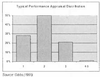
A typical firm conducts annual or semi-annual performance reviews in which super visors give numerical ratings to the workers they oversee. Figure 2.1 displays a rating distribution from a medium-sized service firm in the United States.3 In this firm, 1 is the
rating associated with highest performance, and 5 the worst.
In this firm, almost no workers receive negative feedback: 4 and 5 make up just one percent of the sample. Moreover, there is a marked central tendency in the distribution, with fully fifty percent of workers receiving the rating 2. At the very least, one can
conclude th at managers in this firm do not differentiate between levels of performance as much as the rating scale allows them to. While this distribution comes from only
1 Performance appraisal systems were in place by 300 AD in the Chinese state bureaucracy. As of the early 1980’s, between seventy four and eighty nine per cent of American businesses used them (Murphy and Cleveland 1991).
2The Chief Human Resource Counsel for International Paper recently noted that ’’...few tasks occupy as much time by human resource professionals as designing, implementing, monitoring, and defending performance appraisal systems” (Murphy and Margulies 2004).
T y p i c a l P e r f o r m a n c e A p p r a i s a l D i s t r i b u t i o n
50%
4 0 %
m
0%
Source G tb s (1995)
Figure 2.1: Example of Rating Distribution
one firm, other firms’ rating distributions exhibit similar patterns (Medoff and Abraham 1980, Murphy 1992).
Knowing the true distribution of performance in the firm is impossible, so figure 2.1 taken by itself does not allow one to reach any definite conclusions about feedback. However, there is evidence that it reflects managers’ hiding private information from workers. Several studies have shown that the ratings that supervisors report to workers are significantly higher and more skewed than the ratings they report to independent researchers (see Murphy and Cleveland 1991, p.79, and references therein). Also, the same patterns emerge when rating categories have labels such as “average” and “below average” (Gibbs 1991).4 Finally, workers and managers themselves report that managers do not distinguish among workers.5
The economics and HRM literature has identified several reasons for why there might be limited feedback in organizations. First, managers are very often not rewarded for providing accurate appraisals, so they might not exert the effort required to assess and document the performance of their workers (Baron and Kreps 1999). Second, managers may exhibit favoritism and bias ratings (Prendergast and Topel 1996). Third, organiza tional politics may constrain truth-telling.6 Finally, worker psychology may discourage
4In one particularly stark example, Milkovich, Newman, and Milkovich (2007) report a ten-year study of a thousand-member social service department in which only three of the possible ten thousand ratings were “below average”.
5In a case study of Merck, Murphy (1992) reports such sentiments as “Tell me this, how in the world can 83 per cent of the people be exceeding job expectations while the company, as a whole, is doing just average?” and “How can I rate my people objectively when the other directors are giving all th