5
VIII
August 2017
983
©IJRASET (UGC Approved Journal): All Rights are ReservedMatlab – A Successful Tool for Epidemic Modelling
and Simulation
Ojaswita Chaturvedi
Assistant professor, Department of Electrical Engineering, AISSMS Institute of Information Technology, Pune
Abstract: MATLAB is a widely used platform for all major Engineering, Mathematical and even Biological learning streams. This study focuses on bringing out the capability of MATLAB in the compiler mode to perform successful epidemic modeling simulation. Various mathematical processes have been incorporated in the work to show the epidemic status and the study also includes the building of a basic interactive interface in the compiler mode itself. A collection of epidemic models have been taken from various sources and their simulations have been done in MATLAB successfully to give realistic results. A separate model for Shigella diarrhea has been considered for the building of the basic interactive interface.
Keywords: MATLAB, Epidemic Modelling, Simulation, Epidemic Models, Mathematical Models
I. INTRODUCTION A. Matlab
Ranging from Mathematical, Engineering, Biological and even Chemical, MATLAB has been largely accepted for solving complex problems [1,2]. Epidemic modeling has emerged as a significant tool in the process of disease prevention for which successful modeling and simulation has been achieved through MATLAB [3]. This platform gives a wide range of analytical tools that can be used and extrapolated on the epidemic models to give noteworthy information regarding a particular disease. Enhanced graphical features enable one to think beyond simple analysis and even try further manipulations and uses of epidemic models.
B. Infectious Diseases and Epidemic Models
Transmissible diseases repeatedly produce significant world threats due to the diffusive nature of being transferred from human to human. Such transmissible diseases have accounted for 16% of world-wide deaths in 2008 [4]. In general, such diseases are introduced into a closed population by the insertion of an infective individual or by an external vector [4]. Examples of external vectors include water, air, body fluids, insects such as mosquitoes or biological vectors which carry infectious agents such as protozoa, bacteria or virus.
Disease dynamics can be well understood scientifically using Epidemic modelling. As the risk of infectious diseases is increasing throughout the world, models depicting the respective transmission are becoming more functional. These models are simply tools that are used to predict the infections mechanisms and future outbreaks of diseases. Although many treatment methods are employed across the globe to combat epidemics such as the diarrhoea, many individuals fail to receive or respond to these methods. Thus, the epidemic models focus more on the prevention mechanisms.Karmarck and McKendrick introduced the modelling of infectious diseases in 1927 through the first compartmental epidemic model which consisted of three compartments and came to be known as the Susceptible-Infected-Recovered (SIR) model [5]. The model diagram of the SIR epidemic model is shown in figure 1.
Fig. 1 The Basic SIR Model
The above schematic diagram can be described using a set of ordinary differential equations (ODEs) and some defined parameters.
β represents the infectivity parameter and r is the rate of recovery.
= − (1)
984
©IJRASET (UGC Approved Journal): All Rights are Reserved= (3)
Using the above SIR model as a base, there have been numerous other models that have been formulated since then for various infectious diseases in the continuous perspective. Changes in the number of compartments, the connections between the population compartments and the number of variables included in the model can be varied according to the disease characteristics in order to obtain a new model. The Biomedical Modelling Centre, LA has modelled influenza using the SIR model [6]. This model incorporates factors such as demographics – in/out flow of individuals from the population which make it possible to calculate the incidence rate of influenza for different transmission rates. The University of New South Wales, Australia, has created an agent based model to describe the dynamics of the virus – Hepatitis C that gives rise to liver diseases. Additional inputs such as age, sex and immigrant status help in easily evaluating outputs such as infections, cure and death rates related to the disease [7]. Discrete SI and SIS models have been found to be very useful in determining the dynamical behaviour of diseases such as malaria or gonorrhoea [8].
For this study, we shall consider the SI model as described by Brauer F. [9], the SIS model described by Arino J. [10], the SEIR model of Shah N. H. and Gupta J. [11] and the SIRS model described by Chaturvedi O, Masupe T and Masupe S [12]. These models will all be separately analysed for basic dynamics and simulated in MATLAB to show the variations of population sizes in each class.
II. BACKGROUND A. Epidemic Modelling
For any epidemic, the basic reproduction number is defined as the number of secondary infections caused by a single infectious individual in a closed population. This value is the most crucial numerical aspect of epidemic modeling as it determines the presence and strength of the epidemic, in other words it determines the transmission potential of an epidemic. According to the epidemic
theory, if R0 1 then the epidemic does not exist and if R0 1, and epidemic exists and is likely to spread [13]. The basic
reproduction number can be calculated using mathematical analysis [14], the next generation matrix method [15] or through data analysis [16].
For basic MATLAB simulation, the models have been implemented with assumed parameters. The results that arise from these simulations simply give an overview of the overall change that is expected upon practical execution of the epidemic models.
Simulations have been done for both the epidemic equilibrium (i.e. for values of R0 1) and the case of no epidemic (i.e. for values
of R0 1).
The SIRS model shall be used as a guide to see how the values of R0 have been varied to get results for both the equilibriums.
B. MATLAB Simulation Basics
As outlined in the section above, epidemic models are defined by a set of differential equations which describe the rate of change of each of the compartments with respect to time. MATLAB provides many solvers for differential equations which can be used to solve the set of ODEs for the epidemic model and get the actual number of people in each class over a chosen period of time. The Symbolic Math Toolbox (included in MATLAB from the MATLAB 6.5 version) is extremely a handy tool for solving mathematical problems that involve calculus, linear algebra and mathematical plotting [17].
For solving differential equations in MATLAB, the equation has to be represented using a manually created function and then the solver is used. Single and simple differential equations can be solved using the dsolve function in-built in MATLAB. This solver can be put to use for equations of the first, second and third orders and also for both linear and non-linear systems. If solved with an
initial condition the coefficient is calculated and included in the answer else it is depicted as Cn [18].
When it comes to epidemic models, the model is defined by a system of ODEs (a number of coupled ODEs which are inter-related to each other). The simulation of the system in MATLAB involves the expression of this system in matrix format. The system will
be considered to be a vector x defined as x(y) = [x1(y), x2(y),.., xn(y)] and the derivative of the vector x will be defined as xn= F(y, x,
x’,x’’,…, x(n-1)). Mathematically, the system may not necessarily be linear and considering epidemiology, the human population
985
©IJRASET (UGC Approved Journal): All Rights are Reservedgives more accurate results but for simple calculations, sometimes ode23 is a better option. In this study we have used the ode45 function [19].
III.EPIDEMICMODELSANDSIMULATIONS
All paragraphs must be indented. All paragraphs must be justified, i.e. both left-justified and right-justified.
A. SIRS Model
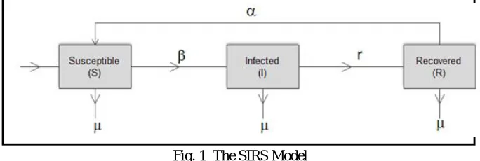
[image:4.612.135.477.224.339.2]This model has been formulated for diarrheal infections caused by the bacteria Shigella. With a small extension of incomplete immunity post recovery, the model is a minute extension of the basic SIR model having the recovered population losing their immunity and becoming susceptible again. The model diagram and the parameter description have been shown in figure 1 and table 1 respectively.
Fig. 1 The SIRS Model
TABLEI
PARAMETER DESCRIPTION FOR THE SIRS MODEL
Parameter Description
Population renewal
rate
β Infectivity rate
µ Natural death rate
r Recovery rate
Immunity loss rate
The above SIRS model can be defined using a set of ODEs as follows:
= − − + (4) = − − (5) = − − (6)
The susceptible population, as the name suggests, is non-resistant to the disease and gets in contact with the pathogen through the infected population. The infected class contributes to the pathogen population in the environment and hence transmits the disease. With the help of medication and rehydration therapies or body immunity, the infectious people become recovered. For some time, the body maintains an immunity level but gradually, this level drops and the recovered population again becomes susceptible to the disease.
The basic reproduction of this model has been evaluated as [12]:
=
( + ) ( )
Considering the borderline situation where R0 = 1, and making the infectivity rate the subject of the formula, the above formula
986
©IJRASET (UGC Approved Journal): All Rights are Reserved= ( + ) ( )
In order to compute the value of the infectivity rate when the basic reproduction is 1, the assumed parameters are fed into equation (ii). Mathematically, it is obvious that the infectivity rate and the basic reproduction number are directly proportional to each other,
therefore considering the value of the infectivity rate calculated in (ii), it is safe to assume that if the obtained value is increased, R0
will become greater than 1 and if the obtained value is reduced, R0 will become less than 1. Therefore, using the computed value of
the infectivity rate, , we can successfully obtain values of R0 for both equilibriums.
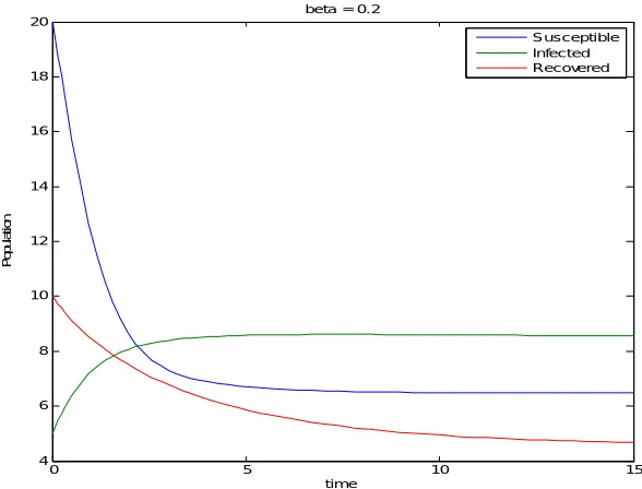
Figures 3 and 4 show the results of the simulations obtained by analyzing the model in MATLAB.
Fig. 3 Simulation of the SIRS Model for the disease free state
[image:5.612.152.446.478.702.2]
Fig 4 Simulation of the SIRS Model for the epidemic free state
0 5 10 15
0 20 40 60 80 100 120 140 160 180 time P o p u la ti o n
beta = 0.0002
Susceptible Infected Recovered
0 5 10 15
4 6 8 10 12 14 16 18 20 time P o p u la ti o n
beta = 0.2
987
©IJRASET (UGC Approved Journal): All Rights are ReservedB. SI Model
The SI model that has been taken up for this demonstration [9] is a special case and alteration of the basic SIR model (figure 1). The system can be shown diagrammatically and expressed through ODEs as follows:
Fig. 5 The SI Model
There are no entries or departures from the closed population that have been considered for this model. The infectivity rate is and r
is the recovery rate which directly makes the individuals susceptible to the disease.
= − (7) = − (8)
The basic reproduction number for this model is defined as
= ( )
Where k = S(0).
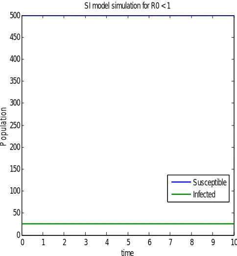
[image:6.612.191.433.416.677.2]Simulations of the model for the disease free and epidemic state are shown in figures 6 and 7.
Figure 6 SI Model Simulation for disease free state
0 1 2 3 4 5 6 7 8 9 10
0 50 100 150 200 250 300 350 400 450 500
time
P
o
p
u
la
ti
o
n
SI model simulation for R0 < 1
988
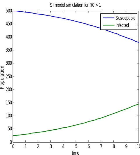
©IJRASET (UGC Approved Journal): All Rights are Reserved [image:7.612.191.431.94.360.2]r
Figure 7 SI Model Simulation for the epidemic state
It is evident from Figure 6 that the population numerical are not disturbed as long as the basic reproduction number is kept below 1. The stagnant values are more dominant in this case due to the absence of any demographic changes. When the basic reproduction number is increased, the susceptible population begins to decrease and the infected population increases. It is noteworthy that the total population remains constant again due to no demographic changes.
C. SIS Model
The SI model described in Figure 5 implemented with demographical changes forms the SIS model that will be considered for this section [10]. Diagrammatic representation of this model is shown in figure 8 and the system of equations with the parameter descriptions is also described following. There will be changes in the basic reproduction number too.
Fig. 8 The SIS Model
Demographic changes ( = population renewal and = natural death rate) have been included in this model. The infectivity rate is
and r is the recovery rate which directly makes the individuals susceptible to the disease. The system of ODEs is listed as:
= − − (9) = − − (10)
The basic reproduction number for this model is defined as
0 1 2 3 4 5 6 7 8 9 10
0 50 100 150 200 250 300 350 400 450 500
time
P
o
p
u
la
ti
o
n
SI model simulation for R0 > 1
[image:7.612.244.363.515.609.2]989
©IJRASET (UGC Approved Journal): All Rights are Reserved=
(+ ) ( )
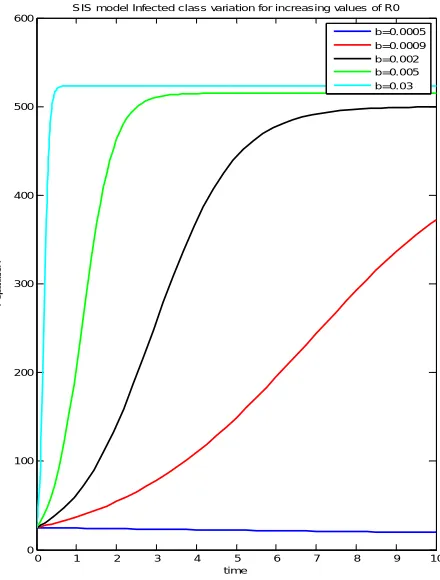
Simulations of the model was done and the graphs for the susceptible and infectious class have been individually shown in figures 9
and 10 for increasing values of R0 which was controlled using the value of the infectivity rate, . It can be seen from the graphs that
[image:8.612.199.429.171.375.2]as the basic reproduction number is increased, the susceptible population decreases while the infected population increases.
Figure 9 SIS Model Simulation for disease free state
Figure 10 SIS Model Simulation for epidemic state
0 1 2 3 4 5 6 7 8 9 10
0 100 200 300 400 500 600 time P o p u la ti o n
SIS model Susceptible class variation for increasing values of R0
b= 0.0005 b= 0.0009 b= 0.002 b= 0.005 b= 0.03
0 1 2 3 4 5 6 7 8 9 10
0 100 200 300 400 500 600 time P o p u la ti o n
SIS model Infected class variation for increasing values of R0
[image:8.612.201.421.413.703.2]990
©IJRASET (UGC Approved Journal): All Rights are ReservedD. SEIR Model
[image:9.612.155.453.196.276.2]For some diseases, there exists an exposed stage. This class is basically the proportion of the susceptible class that has not been introduced to any prevention mechanisms in order to avoid the infections. Such a model formulates to take the SEIR format (Susceptible-Exposed-Infected-Recovered format) [11]. Diagram representation of the model is shown in figure 11 followed by the parameter descriptions and system ODEs. This model also incorporates demographic changes and disease induced mortality as shown and explained in the diagram and the system equations. Permanent recovery (no immunity loss after one infection) is shown in this system indicating that the recovered population never becomes susceptible to the disease.
Fig. 11 The SEIR Model
The population is renewed () and added into the susceptible class. A natural death rate () reduces each class in the model and the
infected class is reduced by an additional death rate due to disease (). An effective infection rate () governs the transition of the
susceptible to the exposed and the regression rate (v) controls the fraction of the exposed class who will be infected. Individuals recover from the disease at a recovery rate (r). The system can be described using the following set of equations:
= − − (11) = − − (12) = −(++ ) (13)
= − (14)
The basic reproduction number for this model is defined as
=
(+ )(++ ) ( )
Simulations of the model was done and the graphs for the susceptible and infectious class have been individually shown in figures
12 and 13 for increasing values of R0 which was controlled using the value of the infectivity rate, .
Figure 12 SEIR Model Simulation for disease free state
0 1 2 3 4 5 6 7 8 9 10
0 50 100 150
time
P
o
p
u
la
ti
o
n
SEIR model s imulation for R0 < 1
[image:9.612.197.422.535.708.2]991
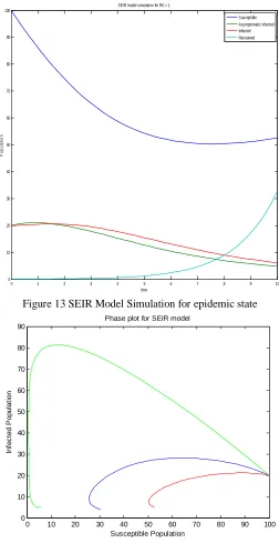
©IJRASET (UGC Approved Journal): All Rights are ReservedFigure 13 SEIR Model Simulation for epidemic state
Figure 14 SEIR Model Phase Plot
We can observe that the changes in each of the compartments for the disease-free and epidemic state show realistic patterns. The susceptible population increases in case of no epidemic and reduces when there is an epidemic. Exposed and infected populations are both expected to rise as shown in the epidemic case. The phase plot analysis (a plot of the infected population against the susceptible population) has also been done for increasing values of the basic reproduction number.
IV.BASICINTERFACEDESIGNFORTHESIRSMODEL
Using the model design and code in MATLAB, together with the pathogenesis of the parasite causing the disease, it is possible to build a basic interface that takes in a few inputs and shows the presence/absence of an epidemic in the defined population. In this
0 1 2 3 4 5 6 7 8 9 10
0 10 20 30 40 50 60 70 80 90 100 time P o p u la ti o n
SEIR model simulation for R0 > 1
Susceptible Asymptomatic infected Infected Recovered
0 10 20 30 40 50 60 70 80 90 100
0 10 20 30 40 50 60 70 80 90 Susceptible Population In fe c te d P o p u la ti o n
992
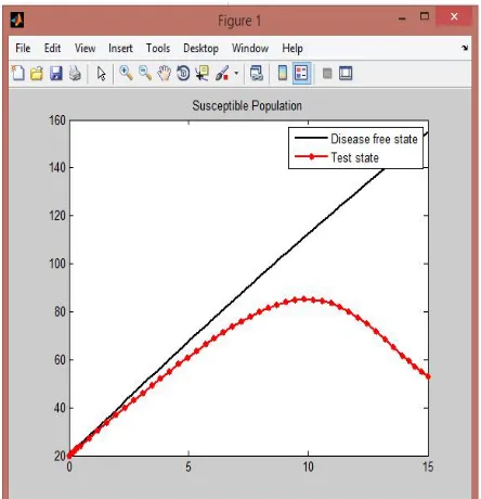
©IJRASET (UGC Approved Journal): All Rights are Reserved [image:11.612.239.386.198.431.2]case, the SIRS model has been considered which has been formulated for shigella. Shigella infections are found out to reach peaks during the summer season [20]. The model takes in inputs of the season (as the month), the population renewal and the natural death rate. Using these values and other estimated parameters, the model is simulated giving out two types of output. Firstly the basic reproduction number is calculated and shown. This numerical value can be directly used to deduce the presence or absence of an epidemic using the epidemic theory. Another output given by the interface is the graphical comparison of the susceptible population of the test state with the disease free state. Figure 14 shows the input prompt and figures 15 to 18 show the output results of the system. Such systems can be implemented on bigger platforms and in this way practical application of epidemic models can be made possible through MATLAB.
[image:11.612.201.423.461.691.2]Figure 15 Input Prompt
Figure 16 Output analyzing the epidemic using the basic reproduction number
993
©IJRASET (UGC Approved Journal): All Rights are ReservedFigure 18 Susceptible Population Variation for disease free state
V. CONCLUSIONS
This work showed that MATLAB can be used very aptly to quantify epidemic models and the results can be displayed in various formats for analysis purposes. Four different epidemic models from previous works were chosen herewith and simulation of each of these was completed successfully in MATLAB. A further extension was shown in the context of epidemic modeling through MATLAB by introducing an interface that can directly provide the epidemic results depending on the inputs entered.
REFERENCES
[1] T. Michalowski, Applications of MATLAB in Science and Engineering, Rijeka, Croatia: In-Tech, 2011.
[2] S. Elnashaie and F. Uhlig, Numerical Techniques for Chemical and Biological Engineers Using MATLAB®, Berlin, Germany: Springer, 2007. [3] H. W. Hethcote, “The Mathematics of Infectious Diseases,” Society for Industrial and Applied MathematicsReview., vol. 42, pp. 599–653, 2000. [4] E. Shim, “An Epidemic Model with Immigration of Infectives and Vaccination,” B.Sc. thesis, The University of British Columbia, Canada, April. 2004. [5] F. Debarre, SIR models of epidemics, Lecture Notes in Modelling course in population and evolutionary biology. Zurich, Switzerland: Institute of Integrative
Biology
[6] B.J. Coburn, B. G. Wagner, S. Blower, “Modeling influenza epidemics and pandemics: insights into the future of swine flu (H1N1),” BMC Med., vol. 30, June, 2009.
[7] A.Agathos. (2017) Kirby Institute, Autralia. [Online]. Available: https://kirby.unsw.edu.au/
[8] L. Jian-quan, L. Jie and L. Mei-zhi, “Some discrete SI and SIS epidemic models,” Applied Mathematics and Mechanics., vol. 29, pp. 113–119, Jan. 2008. [9] F. Brauer, “Some simple epidemic models,” Mathematical Biosciences and Engineering., vol. 3, pp. 1–15, Jan. 2006
[10] J. Arino, Metapopulation models in epidemiology, Presentation for Inner City Health. Centre for Research on Inner City Health, Toronto: Biodiaspora. [11] N. H. Shah and J.Gupta, “SEIR Model and Simulation for Vector Borne Diseases,” Applied Mathematics., vol. 4, pp. 13–17, August. 2013
[12] O. Chaturvedi, T. Masupe and S. Masupe, “A Continuous Mathematical Model for Shigella Outbreaks,” American Journal of Biomedical Engineering, vol. 4, pp. 10–16, April. 2014
[13] P. Holme and N. Masuda, “The Basic Reproduction Number as a Predictor for Epidemic Outbreaks in Temporal Networks,” PLoS One, vol. 10, Mar. 2015 [14] N. Chitnis, Introduction to Mathematical Epidemiology: The Basic Reproductive Number, Lecture notes for Autumn Semester 2011. Swiss Tropical and
Public Health Institute, Zurich, Switzerland
[15] J. H. Jones, Notes On R0, Lecture notes. Department of Anthropological Sciences Stanford University, Stanford, USA: May 2007
[16] A. Cintron-Arias, C. Castillo-Chavez, L. M. A. Bettencourt, A. L. Lloyd and H. T. Banks, “The Estimation Of The Effective Reproductive Number From Disease Outbreak Data,” Mathematical Biosciences and Engineering, vol. 6, pp. 261–282, April. 2009
[17] Mathworks. (2017) Mathworks. [Online]. Available: https://in.mathworks.com/products/symbolic/features.html
[18] M. S. Gockenbach, MATLAB Tutorial to accompany Partial Differential Equations:Analytical and Numerical Methods, Lecture notes, SIAM 2010 [19] C. Moler. (2014) Ordinary Differential Equation Solvers Ode23 and Ode45. [Online]. Available:
https://blogs.mathworks.com/cleve/2014/05/26/ordinary-differential-equation-solvers-ode23-and-ode45/#e82149a3-1a80-4233-93af-914a0c279b14