A review on Compressing Image Using Neural Network techniques

A review on Compressing Image Using Neural

Network techniques

Niharika Krishna1, Pinaki Ghosh2 1

Department of CSECET, Mody University of Science and Technology Lacchmangarh, India 2

Department of CSECET, Mody University of Science and Technology Lacchmangarh, India

Abstract: In today’s day and age the technology is advancing at an exponential rate and our dependence on networks and internet has also increased. Digital images need a massive amount of space for storage. Therefore, the process of transmission of an image from one PC to another PC can be a process which is time-consuming. Therein lies the need for the compression of images. Through this paper we will be discussing the basic concepts of image compression and neural networks and the various techniques that are there for compressing images with the help of neural networks.

Keywords: image compression; neural networks; back propagation neural network; recurrent neural network;

I. INTRODUCTION

The advancement in technology has made the use of multimedia in all fields of computing easier and therefore increasing the use of the multimedia. Images are important documents today but they require a huge amount of space for storage and it’s transmission is thus time-consuming. While this is true that the speed of network has considerably enhanced, and the cost of the disk-storage has declined a lot, new applications that use documents of multimedia type which require a huge data set are unceasingly pushing the boundaries of all these developments. The use of Internet for viewing World-Wide-Web pages is increasing exponentially, while the backbone of networking is not growing anywhere near as fast. Thence, compression techniques will always be just as essential, heedless of the present-day state of the network and the storage technologies.

Image compression has been playing an important part in the storage and transmission of images as a result of the limitations of storage. The main aim of compressing an image is to be able to represent the given image in fewest possible number of bits without the loss of essential data within the original image. Digital image compression is very useful in many important fields such as data storage, communication, multimedia applications, computational purpose etc. Many techniques have been developed to make the storage and transmission of images economical.

Image compression is of two type: lossless and lossy. Lossless image compression essentially means that the all the bits of the image can be recovered after decompression, that is there will be no loss of data. Lossy image compression is the image compression technique wherein some of the bits of the image may be lost while decompressing, that is the image will be very similar to the original image but will not be precisely the original image. One of the most effective techniques used for lossy image compression is with the help of neural networks.

Over the past years, there have been umpteen initiatives to compress images by applying and using techniques of artificial neural networks (ANNs)[1]. Even though artificial neural networks are used in both lossless and lossy types of compression but the use of artificial neural networks in the field of image compression is almost exclusively focused on lossy image compression. This is due to the ability of neural network to provide optimized approximations, noise suppression, parallelism and transform extraction. Research in using neural network for the purpose of image compression is still making steady progress.

In this paper, we will talk over the utilization of various artificial neural network techniques for still image compression and still image decompression.

The leading segments will first talk about image compression and the metrics used to measure the compression of image, and then we will be having a review of some ANN compression techniques and the utilization of ANN to enhance the regular compression methods.

II. IMAGECOMPRESSION

Image compression is done through removing all or some of the following three primary forms of redundancies: Coding redundancy, Inter pixel redundancy and Psycho Visual redundancy. Coding redundancy is related to representing the information or data. A code form is used to represent the information.

It is encountered if number of code symbols used to code the gray levels of an image is more than utterly essential. Inter-pixel redundancy is due to the correlation between the neighboring pixels in an image. For pixels to be highly correlated it should be possible to be able to predict the value of a pixel using the values of it’s surrounding or neighbouring pixels.

The Psycho-visual redundancies are there since the humans do not perceive all the things. The perception of humans doesn’t include the analysis of every pixel at quantitative level or luminance value in the image. Image compression techniques are basically of two types:

A. Lossless Image Compression

Lossless image compression implies that there will be no loss of data of the image while compressing it. It will give a compressed image file but it can be decompressed to get back the original image with all it’s data in original quality. Some of the popular file kinds are TIFF, PSD, PNG, GIF, and RAW.

B. Lossy Image Compression

Lossy image compression is the compression technique where some data (pixels) maybe lost in the process of compressing the image. The image received after decompression process is very similar to the original image but not precisely the original image in quality and other factors. Some of the most common file types are JPG, BMP.

III. METRICSFORIMAGECOMPRESSION

There are multiple ways in which one can express the level of compression that is attained by a particular technique, and the consequent quality received when it is then decompressed.

One of the approaches states compression achieved by giving the total count of bits of the compressed image that are needed to store each pixel in the original image. As this count doesn’t give the original number of bits needed to store all the pixel, outputs or results of compression expressed in the form of bits needed per pixel could be perplexing[3].

Thus we generally use compression ratio to express the compression result. Compression ratio of a compression technique is the ratio of the total count of bits in input or original image to the total count of bits in output image. It is expressed as follows:

image compressed in Bits image original in Bits CR Ratio n

Compressio ( )

This provides a more precise presentation of the compression that has been attained and it is obvious to the variations in grayscale and colored images.

As previously stated, lossy compression techniques give images which on reconstruction are similar but not precisely the same as the original image. For being able to state the quality of the image which has been yielded by lossy compression technique for a particular picture, the Peak Signal to Noise Ratio (PSNR) is used in decibels. PSNR is defined as:

       MSE MAXI 2 10 log . 10 ) Ratio(PSNR Noise to Signal Peak (2) Where MAXI is the maximum pixel value of the image that is possible and MSE is the Mean squared error. Mean squared error gives a squared average of the error that is observed which can be defined as:



Where n is the total number of pixels in image,

Y

Y

ˆ

the value of the input.

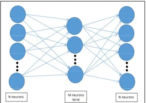
IV. SIMPLEIMAGECOMPRESSIONUSINGARTIFICIALNEURALNETWORK

Fig. 1.A simple neural network based compressor/decompressor

The compression and decompression is done by an individual artificial neural scheme itself. An image block is inputted into the network as input to input neurons and the compressed image can be obtained as the output of neurons of the hidden layer and the decompressed image can be obtained as the output given by the output neurons. Since the input and output has to be same therefore the number of input neurons is equal to the number of output neurons. The number of neurons that are in the hidden layer is lesser as compared to that of the input or output layer. The count of input and output neurons is decided by the size of image block to be entered. For example if we want to input an image block of 8x8 size then 64 of each the input and the output neurons will be needed. Total neurons that are needed in the hidden layer depend upon the compression ratio required. For example if wish to compress the input image block by a compression ratio of 4:1 the we will require 16 neurons in hidden layer as 64:16 = 4:1. Similar to the other feed-forward artificial neural networks this network has to be trained as well so that it can produce useful results. The network is trained in a way so as to produce at output neuron what has been given at input neuron, that is original image block. The output which is given by the hidden or middle layer is taken to be used as the compressed data/image.

V. ANNBASEDIMAGECOMPRESSIONTECHNIQUESANDTHEVARIOUSWORKDONEINTHATFIELD

A. Overview

In this section we will be discussing the various image compression techniques using neural networks. We will be focusing on a few of them, namely Radial Basis Function (RBF), Support Vector Machine (SVM), Back propagation neural network(BP-NN), Recurrent Neural Networks(RNN). Some of the related work done in the respective field is mentioned.

B. Radial Basis Function(RBF)

The Radial basis function network consists of three phase or layer and the traits of every one of the three layers is distinct from the others. The first part or layer consists of the all the input nodes, i.e. source nodes, that connects this layer to the encompassing area. The second part or layer runs in a non-linear transformation and this layer is the hidden layer. The third and final layer gives response on the basis of the given input values and it is the response or output layer which is linear in nature.Arun Vikas Singh [4] has proposed an approach which is a combination formed by utilization of the concept of radial basis function, the vector quantization and the wavelet transform. As we observed here, the image is broken into a many sub bands with different resolutions. The band coefficients with high frequency are compressed with help of of radial basis function. The time needed for computation and PSNR are attained by keeping up a good recovered image.

C. Support Vector Machine (SVM)

A support vector machine(also called support vector networks) is a type of linear machine. It’s primary construction of concept can be explicated as in the scenario of divisible patterns which originate in the circumstance of pattern recognition.[6] It is basically a supervised learning model that uses associated learning algorithms which analyses data for it’s classification analysis.

This model is a representation of the examples points that are mapped in space such that the points of different categories separated by gaps and are as far as possible. The new example points are mapped onto the same space and prediction is done as to which category they belong to on the basis of which side of the gap they lie. A hyper plane is built by support vector machine and for that it separates the positive items to one region and the negative items to the opposite region of the margin. Consequently, the SVM will do very well in the case of issues relating to classification of pattern. It will not be integrating domain information related to problem[7]. That particular property is exclusively in support vector machines.

Fig. 2.A general diagram of SVM

In terms of the time-period, support vector machines presently are more time taking as compared to the other neural networks for similar generalization performance but in a comparison of SVM, Radial basis function and Back propagation network done for image compression by using medical images as the input images the result was positive if not time saving. In the end, by carefully evaluating every parameter via setting various images as the inputs of the three different algorithms it was decided that the support vector machine was the most effective among them[6].

D. Back Propagation(BP) Neural Networks

In image compression technique using back propagation artificial neural network three layers are defined, an input layer, a hidden layer and an output layer. Both the input and the output layers are attached fully to the hidden layer, i.e. fully connected. Compression of the image has been achieved by scheming the count of neurons in the input and the output layers to be lesser as compared to that of the neurons in hidden layer.

The BP neural network may be a linear type or a non-linear type neural network depending upon the transfer function working in the layers. One of the most common functions used in various neural network is the Log-sigmoid function given in equation (4).

) exp( 1

1 )

(

x x

f

  

(4) Several neural networks use the log-sigmoid function as the transfer function for the hidden layer and a linear function is used in out put layer as transfer function. Non-linear functions have the ability of learning the linear and non-linear jobs both, rather than the linear ones. The output value at the hidden layer for jth neuron is calculated by using equation(5).







 _in ij j

j f w b

z 1 ₁



_



 m

l kl l k k f w z b y

1 2

(6) In equation (5) f1 is the function of the hidden layer and in equation (6) f2 is the function of the output layer.

D. Likith Reddy and DSC. Reddy[8] proposed a feed forward back propagation technique for image compression by using only single training set and significant improvement in compression ratio and peak signal to noise ratio was observed. Modularity is provided in the structuring of the architecture of the network due to the adaptive characteristics of the approach which is less susceptible to failure and easy for rectification and it also speed up the processing.

Birendra Kumar Patel[9] proposed an image compression technique which utilizes the back propagation neural network and also combining the Levenberg-Marquardt concept with it. The first step is to divide the input image into various blocks and every sub-block is then passed to the network based upon the complexness of the value of sub-sub-block. The Levenberg-Marquardt algorithm in combination with the back propagation neural network showed that compression of image and convergence time can be bettered. An adaptive approach has been proposed by Prema Karthikeyan[10] by changing the training algorithm of the back propagation network with Levenberg-Marquart method. Modified Levenberg-Marquart concept is used for selecting images that have to be compressed. This approach uses different networks for different input image blocks according to their complexity values. The experimental results show that a better quality of image is received by overlapping neighboring image blocks.

A hybrid intelligent learning algorithm is proposed by Jia Wei[11] based on a combination of genetic algorithm and back propagation algorithm which not just overcomes the defects of local convergence of back propagation algorithm and less convergence speed, but it also solves problem of finding global optimal solution when using genetic algorithm separately. The effect of training using this method has been better than that of the training method solely or that of the evolutionary genetic algorithm, training of the feed forward network by using it for doing compression of grayscale image has produced excellent compression effect.

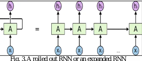
E. Recurrent Neural Networks(RNN)

Recurrent neural networks are formed by looping of connections or connection is such that is forms a directed cycle. Unlike the feed-forward neural networks, RNNs can use their own internal memory to process sequences of arbitrary inputs.

Fig. 3.A rolled out RNN or an expanded RNN

An RNN based image compression method was proposed by G. Toderici et al.[12] which gives a method for variable-length encoding of image patches. The neural network architecture share the same conceptual stages: an encoder network, followed by a quantizer, and then a decoder network. Additionally, this framework is tuned for image compression and supports variable compression rates without the need for storing multiple encodings of the same image. Multiple copies of the residual auto encoder are chained together. This chaining is explict.

VI. CONCLUSION

This paper has discussed image compression and image compression techniques using artificial neural networks. It has focused on SVM, RBF, BP neural network and RNN techniques and the various advancements done it that particular network.

conclude that by modifying it using other algorithms we can improve that[9]. We can deduce that using RNN model has it’s advantages like somewhat reduced inter-block boundaries, deflecting undue smoothing while removing block artifacts and maintaining the balance between saving the real details and avoiding smearing of color but it may lead to disadvantages like increased bleeding of color or introducing encoding artifacts at patch boundaries[12].

It is concluded that although all of them have advantages and disadvantages as compared to each other the area of their application majorly dominates the decision as to which technique is the better one. Each of the technique is useful in different applications and thus are effective. There is possibility for further improvement in the CR and PSNR values of the SVM, RBF, BP and RNN compression techniques by combining other algorithms already in play.

REFERENCES

[1] V. R. P. Vaddela and K. Rama, “Artificial Neural Networks for Compression Of Digital Images : A Review,” Int. J. Rev. Comput., pp. 75–82, 2010. [2] S. Yadav and S. Singh, “A Review on Digital Image Compression Techniques,” Int. J. Adv. Res. Comput. Eng. Technol., vol. 4, no. 9, 2015.

[3] Christopher Cramer, “Neural networks for image and video compression - A review,” Eur. J. Oper. Res., vol. 108, no. 2, pp. 266–282, 1998.

[4] A. V. Singh and S. Murthy K, “Neuro-Wavelet based Efficient Image Compression using Vector Quantization,” Int. J. Comput. Appl., vol. 49, no. 3, pp. 32–37, 2012.

[5] A. Alexandridis, E. Chondrodima, and H. Sarimveis, “Radial basis function network training using a nonsymmetric partition of the input space and particle swarm optimization.,” IEEE Trans. neural networks Learn. Syst., vol. 24, no. 2, pp. 219–230, 2013.

[6] B. Perumal, M. P. Rajasekaran, and H. Murugan, “Comparison of neural network algorithms in image compression technique,” Int. Conf. Emerg. Technol. Trends, pp. 1–6, 2016.

[7] J. Yang, J. Xie, G. Zhu, S. Kwong, and Y. Q. Shi, “An effective method for detecting double JPEG compression with the same quantization matrix,” IEEE Trans. Inf. Forensics Secur., vol. 9, no. 11, pp. 1933–1942, 2014.

[8] D. Likith Reddy and D. S .C. Reddy, “Image Compression Using Feed Forward Neural Networks,” Int. J. Eng. Sci. Res. Technol., vol. 6, no. 3, pp. 143–148, 2017.

[9] B. K. Patel and Prof. S. Agrawal “Image Compression Techniques Using Artificial Neural Network” International Journal of Advanced Research in Computer Engineering & Technology, Vol 2, October 2013.

[10] P. Karthikeyan and N. Sreekumar, “A Study on Image Compression with Neural Networks Using Modified Levenberg - Maruardt Method,” Glob. J. Comput. Sci. Technol., vol. 11, no. 3, 2011.

[11] J. Wei, “Application of Hybrid Back Propagation Neural Network in Image Compression,” in International Conference on Intelligent Computation Technology and Automation (ICICTA), 2015.