3 4 13h Hybrid Simulation of a Temperature Rate Flight Control System for Re Entry Vehicles 1965 pdf

HYBRID SIMULATION OF A TEMPERATURE RATE FLIGHT CONTROL SYSTEM FOR RE-ENTRY VEillCLES

INTRODUCTION

This Study describes a six - degree -of-freedom

hybrid simulation for the optimum design of a space vehicle re - entry flight control system, utilizing the E A I HYDAC ® 2400 Combined Hybrid Computing System. The specific purpose of the simulation is the evaluation of a tempera-ture-rate flight control system (TRFCS) which utilizes temperature sensors to provide short-period stabilization and long - term guidance during atmospheric re-entry.

During the past ten years, a great deal of research and development work has been conducted on various types of re-entry vehicles and numerous techniques for guiding and controlling such

vehicles have been proposed. The new flight

control system described here is, by its nature, simple and reliable, and inherently insures a safe re - entry. The ensuing discussion explains the

general re-entry problem and the unique control system being studied, and includes a detailed discussion of the simulation equipment required

and its programming.

GENERAL RE-ENTRY CONSIDERATIONS To obtain a better insight into the need for a

simple yet reliable guidance and control system

[image:1.615.9.598.9.759.2]

/ ... TEMPERATURE SENSORS

Figure 1. Sketch of Re·Entry Vehicle

for lifting re-entry vehicles, abrief discussion of the general re-entry problem follows.

The re-entry vehicle utilized in the study (and shown in Figure 1) is an unpowered lifting vehicle

with wings which, unlike its ballistic counterpart, is highly maneuverable and can be landed on

conventional runways.

The lift and drag coefficients (CL and CD) of. a

typical high LID lifting re- entry vehicle are shown in Figure 2 as a function of angle of attack. A plot of lift to drag ratio (LID or CVCD) is also shown since it is of importance in deter mining the range of the re-entry vehicle. During the high

velocity portion of re-entry flight the vehicle operates on the high CL (large cc) side of (LID) max. (150

< <X < 65°). These larger lift coefficients

yield a re-entry trajectory with lower dynamic

pressure, acceleration, and temperature. Figure 3 shows a typical uncontrolled re-entry trajectory

with a angle of attack, oc , of 35 deg. Figure 4

defines the coordinate system and symbol.

o

0.7

10 20 30 40 _.0 00

C)( -ANOLl 0' ATTACk

During most of the vehicle flight, ro + h '" ro and

t" '" o. Thus, the following approximate equations

can be used:

000

LOCAL HORIZONTAL

~4 y2 L

h"'-g+r-;;-+ffi

V"'-~

" .. HO[- THOUSANDS OF NAUTICAL MILES Figure 3. Typical Re-Entry Trajectory

GLIDER LONGITIIOINAL

v

h

(1)

(2)

h - ALTI TilDE 1\ -FLIGHT PATH ANGLE (APPROXIMATELY ZERO)

ro - RADIIiS OF EARTH 0<. -AHGLE OF ATTACK

r - ro+h:::: ro LIM-LIFT ACCELERATION

V .- VEHICLE VELOCITY DIM -DRAG ACCELERATION

Figure 4. Simplified Planar Re-Entry Coordinate System

For a lifting r,e-entry vehicle, the lift is large enough to allow the vehicle to fly along an equil-ibrium glide path where h'" o. Along this path-,

L g _ y2

c~

SCL (3)

m r ' m

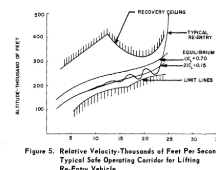
where q is the dynamic pressure (1/2 pV2) and S is the wing area. Thus, for a given CL, there is a unique altitude-velocity profile. Figure 5 shows the altitude - velocity profile for two different

equilibrium glide lines and the boundaries of the re - entry corridor. The lower boundary of the corridor is determined by the temperature and load limits of the vehicle and the upper boundary by the recovery ceiling. The recovery ceiling is defined as that altitude (with altitude rate,

11

=

0) from which the vehicle can recover without

exceeding the temperature and load limits of the vehicle.

~

""

~

.... 0

c z

~

~

0

:z:

t;-""

0 ~ ~

i=

-J

"'

500

TYPICAL

400 RE-ENTRY

300

200

100

10 15 20 25 30 35 Figure 5. Relative Velocity- Thousands of Feet Per Second

Typical Safe Operating Corridor for Lifting Re-Entry Vehicle

One of the primary re-entry problems is in keeping control of the vehicle so that temperature and load limits are not exceeded and that a smooth equilibrium glide is established. The heavy trajectory shown on Figure 5 is a typical uncon-trolled re-entry with its familiar skipping oscil-lations which cause the vehicle to approach dangerously close to the heat limits. The temperature rate control system being simulated was developed to eliminate these skipping oscillations and to reduce the peak temperatures duril1g re-entry.

Another re-entry problem is in carefully managing the energy of the vehicle as it re-enters so that the desired terminal pOint is reached. The range capability of the re-entry vehicle can be deter-mined quite readily in the re-entry portion of flight since the vehicle is near equilibrium glide where h ~ O. If both sides of Equation 2 are divided by L / M or g - V2 / r, the following is obtained:

V

D

- - 2 = L

g-~

ro

If

V:

is substituted for

V:

ro YdY dR = (LID) - 2

-Y - rog

(4)

[image:2.629.79.302.86.578.2] [image:2.629.324.545.158.331.2]

If this is integrated from an initial velocity to zero, the range is obtained:

R

~ (~\

In ( _ 1

2)

2 \D)

~

- V

(6)

r~

Thus, during the re-entry portion of flight, the range is a function of velocity and LID. Range control is accomplished, then, by varying LID,

Le., by varying the angle of attack. From Equation 6 it should also be noted that the range is very sensitive to initial velocity when the velocity is nearly equal to orbital velocity, yr;g. For the re-entry shown in Figure 3, for example, the sensitivity of range to initial velocity error is approximately 80 NM/fps.

Lateral maneuverability is obtained by banking the re-entry vehicle so that the aerodynamic lift vector is rotated, providing a lateral acceleration.

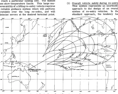
Figure 6 shows an energy management footprint for a typical re-entry flight. The lines of constant

0:: and f1 show what attitude must be maintained

to reach a particular landing site. The dashed lines show temperature limits. This large ma-neuverabilityof a lifting re-entry vehicle requires a reliable guidance system which will perform accurately over the long re- entry, and will minimize errors at the desired terminal point.

U 88R

CHINA

1:\·

~ "',

30·

'\j

~

4:\·

lOS- 120· 13S· ISO· ISS· 180· 16S·

The temperature rate control system is being simulated to demonstrate its compatibility with different types of navigation and guidance systems. As will be pointed out in the next sections, the TRFCS acts as a filter to the guidance signals to insure the safety of the vehicle at all times.

STATEMENTS OF THE PROBLEM

Problem Objective: The temperature rate flight

control system (TRFCS), developed by the AC Spark Plug Division of the General Motors Cor-poration, is based upon the use of temperature sensors instead of conventional inertial instru-ments to provide both short-period stabilization and long-term guidance duringthe re-entryflight. Details of this flight control system are given in the AC Spark Plug Report (1). The mathematical formulation for the simulation of the re-entry problem was furnished by AC Spark Plug.

The new control system introduces several Significant advantages:

ISO·

(1) Overall vehicle safety during re-entry. This system represents an unorthodox approach to the design of an overall system of re-entry vehicles. In the standard approach, the tendency has

- - + - - - 1 - - - ' _ o _ _ - - - 11:\.

13S· lOS· 90· 1S· 60·

[image:3.615.77.532.319.684.2]

been towards a complex integrated system. In the TRFCS, a successful effort has been made to separate safety of the vehicle from the task of accurate navigation. Because of the inherent nature of temperature rate feedback and certain selected lim its . on the control authority, the control system minimizes skin temperature peaks. The maximum "g's" and dynamic pressure are independ-ent of initial conditions and maneuvers performed. This safety aspect of the TRFCS performance is entirely inde-pendent of the guidance commands and, in fact, the TRFCS serves essentially as a filter for them.

(2) Simple, reliable hardware. This separation of control and guidance also results in more reliable hardware since the failure of the necessarily complex guidance system cannot cause the complete destruction of the vehicle. Furthermore, simple thermocouple temperature sensors replace the conven-tional gyros and accelerometers. These sensors are used to control the flight path as well as the short-period oscillations in pitch and yaw. The only additional sensor required, besides the temperature sensors, is a vertical reference gyro which, for the safety aspects of the re-entry, can be quite inaccurate.

(3) Both manual and automatic modes. In case of automatic guidance system failure, the TRFCS can be controlled manually. The manual flight program to be followed by the pilot is very simple, and the resulting temperature peaks, dynamic pressure, and "g"loads compare favorably with those obtained in the fully automatiC mode.

During past years, extensive simulation studies were conducted by AC Spark Plug to obtain familiarity with the control system. A rather conventional simulation program was pursued: first, analog simulations were performed to gain qualitative knowledge of the system, and to determine the practibility of this approach; second, digital tec·hniques were used to eValuate the accuracy of the guidance through TRFCS.

In the analog simulations, the system character-istics were split and analyzed in two indep~ndent

studies. In the first, a three-degree-of-freedom simulation of the mass center of the vehicle was combined with equations describing the

short-period pitch dynamics of the vehicle. Pitch axis controls and trajectory controls in three dimen-sions included an approximate, simple lag representation of the lateral response of the vehicle. In the second type of Simulation, the effects of lateral dynamics were obtained by simulating the dynamics of the vehicle in detail by a standard set of lateral stability equations with variable coefficients. The coefficients were varied with dynamiC pressure, velocity, and stagnation temperatures of the vehicle skin, all obtained from function generators. The data for setting up the function generators came from the first type of simulation. In turn, the results from the second type of simUlation were used to determine the lumped lateral response for the first type of simulation. Thus, a basis for an iterative procedure was established.

The reason for separating the simulation of the pitch dynamics and trajectory control from simulation of the lateral dynamiCS was the unavailability of necessary simulation equipment. The investigation of aspects of the system such as coupling between pitch and roll could not be made with the above "split" simulation approach and required a complete six-degree-of- freedom simUlation.

The next logical step} therefore, was to study the system I s characteristics in a combined

six-degree-of-freedom simulation. Here the question arose of what computer or computers should be used. Past experience had shown that the conventional first-analog - then -digital approach was definitely not the best. Some of the conclu-sions gathered during past simulations are as follows:

(1) Repeatability of analog simulation was only marginal (50 miles in range).

(2) Slowness of digital simulation. Even for narrow ranges, determined by previous analog Simulation, digital simulation was too time consuming and, therefore, too expensive to optimize parameters. Reduction of the digital data also proved to be a problem.

Problem Background: The main obj ective of the

required. Economy of analysis should be consid-ered, especially in the automatic guidance studies, where faster-than-real .. time simulation can be

employed.

Computational Requirements: In order to attain the above problem objective, the following set of rigid computational requirements must be met:

(1) High accuracy in traj ectory calculations for the evaluation of the guidance capability of the TRFCS.

(2) Very fast computing capability to simulate the high frequency parameters faithfully for the short-period dynamics of the vehicle.

(3) Real- time and faster - than - real-time simulationfor control system evaluation. (For economical evaluation of the control system in automatic mode, the time scale should be as high as possible.)

On the basis of experience gained during past Simulations, it was concluded that the simulta-neous need for high accuracy and very fast computation can only be satisfied by a hybrid digital-analog computer. Such a computer would allow the programmer to choose either analog or digital solution for different portions of the problem, trading it with fast processing for high resolution, etc.

231R -v ANALOG COMPUTER I. FAST ANALOG

COMPUTING, COMPONENTS 2. ANALO(i MEMORY 3. HIGH SPEED

MODE CONTROL 4. FAST, ACCURATE

FUNCTION GENERATIONS

350 DIGITAL OPERATIONS SYSTEM I. PROGRAMMABLE

LOGIC 2. HIGH SPEED

~ CONVERSION

f----EQUIPMENT 3. CLOCK AND COUNTERS 4. INTERFACE

f4- 5. PARALLEL COMPONENTS 14-MEMORY

6. HIGH SPEED TWO- VARIABLE FUNCTION GENERATION

DIGITAL COMPUTING SYSTEM 375

(3C ODP-24)

I. HIGH SPEED ARITHMETIC OPERATIONS 2. FAST RANDOM

ACCESS MEMORY 3. STORED PROGRAM OPERATION 4. EXTENSIVE

INPUT-OUTPUT CAPABILITY

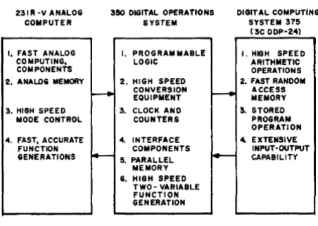
Figure 7. HYDAC 2400 System Configuration

The HYDAC 2400 Combined System, comprising a P ACE® 231R-V Analog Computer, a series 350 Digital Operations System (DOS), and a Series 375 Digital Computing System, was used to perform this simulation. Figure 7 shows a block diagram of this system.

Selection of the HYDAC System enabled the programmers to use analog and digital computing equipment judiciously and to produce the best mechanization of the problem.

PROBLEM MECHANIZATION

All the advantages of hybrid computation are in vain unless very careful consideration is given to the programming of the physical system under study. This phase of the simulation transforms the essentially general purpose computer into a simulator of the specific physical system.

Allocation 0/ Tasks: The first step towards a

successful hybrid program is the allocation of tasks on the computer. The underlying philosophy is to subdivide the physical system into sections and to assign these to various parts of the computer where their speed and accuracy needs are best satisfied. As shown in Figure 8, the physical system consists of four sections, three of them (the vehicle dynamiCS, the TRFCS, and the temperature sensor simulation) constituting the attitude control loop, while the vehicle dynamiCS (together with the guidance system and TRFCS) form the long period loop.

I VEHICLE _::I TEMP. SENSOR

I

I DYNAMICS _I v SIMULATION

<-LONG PERIOD SHORT PERIOD

LOOP LOOP

r GUIDANCE l I _{TR FCS}

SYSTEM

r

_{1 I}

Figure 8. The Physical System

The assignment of these sections to various elements of the HYDAC 2400 computer is shown

in Figure 9. (Compare with Figure 7 for task vs. function assignments.) The attitude control loop, conSisting of the vehicle rotational dynam iCs, the TRFCS, and the short period sensor equations, are programmed on the analog section. In addition, the displays and cockpit simulator are tied into the analog since continuous analog signals are required. The translational equations of motion, long period heat sensor equations, and guidance equations are programmed on the 375 because of the stringent accuracy requirement. The DOS 350 provides the master timing, data conversion, function generation, and reaction jet control logic.

[image:5.617.310.530.332.407.2] [image:5.617.65.291.388.548.2]

231 R-V ANALOG COMPUTER I

350 DIGITAL OPERATIONS SYSTEM

t

-, -

-I-I

I

ri,

SHORT TERM I'---.J

I

I VEHICLE DYNAMICS

J.---I I

I

I

I

I

SHORT TERM _{TEMP. SENSOR}

j---

I

SIMULATION

1

-I

I I I I

~

I

TRFCS I

~

1

I

I I

I

--t

COCKPIT

_j;bL

I DISPLAYS _I

I

DIGITAL COMPUTING SYSTEM 375

I

TRANSLATIONAL

ADC _I EQUATIONS

,

I OF MOTION

I

,

I

I

I

1

I

I LONG TERM TIMING

AND

-

r- ' - - - - I -

f--TEMP. SENSOR

CONTROL

I

SIMULATION

,

I

I I

I

~

I

I I

:Qj~: I

I

-_._.

I

J GUIDANCE

I

CH~~LS

,SIMULATION I

I I

I I

I FUNCTION)~ I LEGEND

I GENERATIONS I CONTROL LINES

I I

DATA LINES _ _ _ _

Figure 9. Block Diagram of Complete System

The DOS, through its timing and controls, syn-chronizes the calculations on each computer and controls the flow of information between sections. Function generation and the reaction control jet logic are ideally suited to the DOS since these operations can be performed rapidly in parallel with the general purpose digital computer so that the digital computation time is minimized.

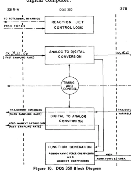
DOS 150 Program:. Figure 10 shows a detailed

block diagram of the DOS. The DOS performs the five following functions: 1.) Timing, 2.) Mode Control, 3.) Data Transfer, 4.) Function Gen-eration, and, 5.) Reaction jet control logic. These functions are descr ibed in detail in the following sections.

1. Timing

Timing is required on a hybrid computer for the following reasons:

(1) To make the mathematical time step used in the integration in the digital progl?am correspond to the physical time scale used on the analog computer; i. e .. -, to make the digital and analog sections run in synchronism. This synchronism is accomplished by sending a periodic

master time pulse, Tl, which initiates the calculations for each time step in the digital computer.

231R-V

I TO ROTATIONAL DYNAMICS

_._._._--I

~-~~-.-•

I

0<. ,/3,j.L ,. cf E

( FAST SAMPLI~G RATE)

•

I I

I

DOS 350

REACTION JET CONTROL LOGIC

ANALOG TO DtGITAL CONVERSION 375 I I I lot.B,A _--L--- ---1----I

TRAJECTORY VARIABLES (SLOW SAIIIPLING RATE) AERO. 1II0lllENT eo FORCE C (FAST S Alii PLI NG RATE

I TRAJECTORY

- - - - -

---.-~-+--'---=---::-::-• VARIABLES

DIGITAL TO ANALOG CONVERSION

FUNCTION GENERATION

I I

AERODYNAIIIIC FORCE COEFFICENTS MACH

AND '""A~E-RO-. F""'O""R"-C E-'-C-OE-F.--MOIII E NT COEFFICENTS

[image:6.620.78.534.46.323.2] [image:6.620.315.541.392.687.2]

(2) To time information transfers between the analog. section and the digital section. Not all transfers are at the same rate since the serial memories of the DOS are used for function generation of aero-dynamiC moment and force coefficients.

These variables must be transferred at a high rate since the functions are used in the short period rotational dynamiCS of the system. On the other hand, those variables relating to long term traj ectory variations are transferred to the digital section at alower sampling rate. Timing is clearly needed to control these two different transfer rates.

1 - - - -AOC XFER I - - - O A C XFER

1 - - - -START CYCLE (T 1) 1---r~r-r-T"J"--rJr' (20 P P S)

INPUT PULSE --~

(500 PPS)

BINARY CODED DECIMAL COUNTER

Figure 11. Master Timer - Block Diagram

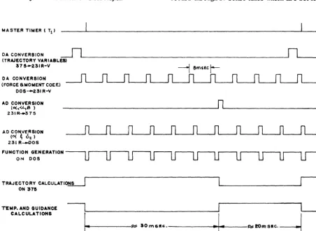
Timing is controlled from the DOS with a Master Timer which controls the sequence of events occurring per cycle of operation. The master timer is a BCD counter driven by the 5MB signals occurring at the rate of 29 pps (approximately one pulse every 2 ms.) Figure 11 shows a block diagram of the master timer.

As shown schematically in Figure 12, events are scheduled with respect to the master timing signal, Tb (every 25 5MB's), the transfers AD andDA being initiated at the specified times TAD and TDA respectively. At the end of one compu-tation cycle, the digital program jumps to the main executive loop and waits there until T1 is received. In this manner, the digital section can be run synchronously with the analog. For instance, if T1 occurs every 50 ms and the time scale desired is 2.0 times real time, the time step to be used in the digital program is 0.1 sec.

2. Mode Control

A very important function of the DOS 350 is to control the modes of operation of the system. Communication between the DOS and the 375 occurs through 16 sense lines which are set from

OACONVERSION ~L-__________________________________________________ ~r-l

_____ _

(TRAJECTORY VARIABLES) 37S-Z3IR-V

DA CONVERSION (FORCE aMOMENT COEF.)

00S-Z3IR-V

---j

smSEc

r-AD CONVERSION

(Q(,.u.,S )

_____________________________

~n~

_________________ _

231R ... 375

AD CO,\VEASION

(0( ., cS_{E )}

23IR-DOS

FUNCTION GENERATION

ON DOS

TRAJECTORY

CALCUL.ATlO~

ON '375

~

__________

~r--TEMP. AND GUIDANCE

CALCULATIONS

I

I

L

\III~I---:~

10 m

6.~.

---t

..

~1

*_----""lOm sac.

---I

[image:7.623.83.536.349.679.2]

the DOS and sensed on the digital section. In the other direction, eight flip-flops on the DOS can be set from the 375 with special OCP instructions (output control pulses). Of these, four can also be reset from the digital console.

All modes are controlled by pushbuttons from the DOS 350 and the following list summarizes the state and function of the analog and digital sec-tions when the indicated pushbutton is depressed.

(1) I C (initial condition) a. 231 R in IC b. 375 in IC

In IC the 375 goes through all computations with the exception of the integra tion routine.

(2) TIC (type in intital conditions) a.231Rin1C

b. 375 is ready to accept new initialization data from the typewriter. From this mode the program returns automatically to the IC loop.

(3) TYTI (type titles) a. 231R in IC

b. The 375 types out title block and line headings for the 26 variables chosen for print out.

(4) TRA (transfer only) a. 231R in IC b. 375 in IC

This mode is for single stepping through the DA and AD transfers and was found very useful for problem checkout. The Master Timer is stopped and now in-cremented only manually by pushbutton action. The data is transferred in both directions, one word at a time, each time the pushbutton TEST CONV is de-pressed. After completion of the DA transfer, the di-gital program jumps to the executive waiting loop (EXWL) where it waits for another master timing signal from the appropriate pushbutton.

(5) DA Test Pattern a.231Rin1C

b. The 375 goes directly to theDA transfer and back to the EX WL, skipping all calculations. A fixed block of data consisting of positive and negative maximum values (corresponding to ± lOOv on the analog) is transferred continuously. This was found very con-venient for a quick check 0 {the DA conversions.

(6) OP (operate) a. 231 R in operate b. 375 in operate

This is the normal mode of operation of the system.

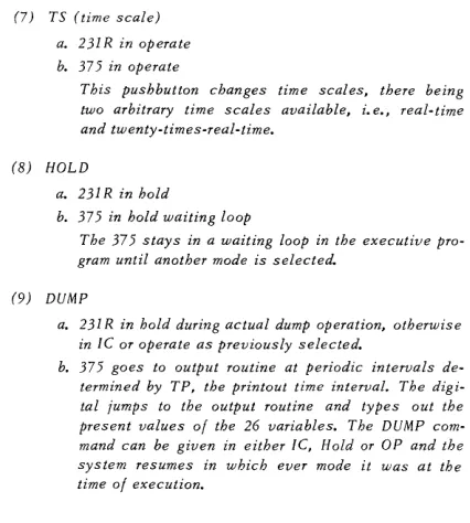
(7) TS (time scale) a. 231R in operate b. 375 in operate

This pushbutton changes time scales, there being two arbitrary time scales available, i. e., real-time and twenty-times-real-time.

(8) HOLD

a. 231 R in hold

b. 375 in hold waiting loop

The 375 stays in a waiting loop in the executive pro-gram until another mode is selected.

(9) DUMP

a. 231 R in hold during actual dump operation, otherwise in IC or operate as previously selected.

b. 375 goes to output routine at periodic intervals de-termined by TP, the printout time interval. The digi-tal jumps to the output routine and types out the present values of the 26 variables. The DUMP com-mand can be given in either IC, Hold or OP and the system resumes in which ever mode it was at the time of execution.

3. Data Transfer

The data transfer for this problem is very demanding since two basic sampling rates are required, one for the short period aerodynamiC functions and the other for the long period tra .. jectory variables. The data transfers will be discussed in two parts: 1.) the analog-to-digital conversion and 2.) the digital-to-analog conver-sion.

a. Analog-Io-Digital Conversion • .• Two variables, a

and 0 E' are converted every 5 millisec-onds since they are used on the DOS for function generation. Once every 50 milliseconds, a ,{3 ,

and f.L are converted and transferred to the 375 for use in the long period trajectory calculations.

Figure 12 in the previous section shows these two different types of conversions.

Figure 13. ADC Data Transfer - Block Diagram

[image:8.613.325.538.51.288.2] [image:8.613.330.524.529.603.2]

When the conversion is complete, the converted data is either loaded into a serial memory on the OOS for use in the function generation program or sent on to the 375 for use in the digital calcula-tions. The data transfer from the DOS to the 375 is accomplished by loading the data into the buffer register and setting the parallel input charmel ready flip -flop on the digital computer. This flip-flop is enabled from the DOS by a pulse on the TEiline prior to each A-D transfer. The 375 then inputs the data through its parallel input charmel. It can be seen that the DOS controls all the A - D conversion, thus minimizing digital computing time on the 375.

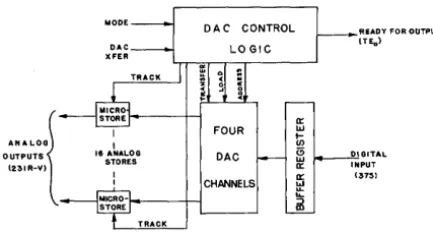
h. Digital-to-Analog Conversion • .• Updated values of the

aerodynamic' force and moment coefficients which are generated on the DOS are transferred to the analog every 5 milliseconds. The trajectory variables (altitude, temperature, guidance errors, etc.) are transferred from the 375 to the analog once every 50 milliseconds. Figure 12 in the previous section shows the timing of these transfers.

A block diagram of the DAC data transfer is shown in Figure 14. The digital-to-analog transfers are initiated by the DOS control logic upon command from the master timing. If data is to be trans-ferred from the 375, the DOS sets the output channel ready flip-flop on the 375. This flip-flop is enabled from the DOS by a pulse on the TEo line prior to each D-A transfer. The 375 will then

ANALOG!

OUTPUTS (231 R-V)

I

16 ANALOG

STORES I I

DAC CHANNELS

READY FOR OUTPUT

(TEoI

INPUT

(37~)

Figure 14. DAC Data Transfer - Block Diagram

output information to the buffer register and the DAC logic on the DOS loads it into the proper DA converter. To minimize digital computer time on the 375, four data words are loaded into the four DAC's (under the control of the DOS). While this data is being converted and then demultiplexed on the analog under control of the DOS, the 375 is formatting the next four words to be transferred. This process is repeated until all sixteen words are transferred. USing this technique, the total processing time consumed for the transfer operation (exceptfor formatting) is only 200 flsecs. The force and moment coefficients are transferred by loading the four DAC's from the serial memories which store the latest computed values

of these coefficients. The data is then converted and demultiplexed on the analog and then the last four coefficients loaded. The DOS controls these conver sions so that they occur at the end of each function generation period and therefore do not interfere with the conversions from the 375 to the analog.

4. Function Generation

The present simulation requires the generation of eight aerodynamic force and moment coefficients. Among these are four functions of one variable ( C 7Jf3 (oc), C 113 (oc), C 11& (a:), C 100 (oc», and four functions of two variables, (Cm(0::,8E)' CL( 0::, M), CD( 0:: , M), Cy f3 (0::, M)). 0::, M, and 8 E are angle of attack, mach number, and elevator deflection respectively. These functions are generated on the DOS for the following reasons:

(1) The functions of two variables are extremely difficult to generate in the analog section and would, at best, require a number of sums and products of functions of one variable. The functions of one variable could be generated on the analog but were programmed on the DOS because of the ease of setup and the speed at which the functions could be changed to study other vehicle config-urations.

(2) The functions are also very difficult to generate on the 375 because of the fast sampling rate required. The sampling rate on the functions should be at least 10 samples per second since they are used in the short period attitude loop of the vehicle. In the real time Simulation, the functions should therefore be sampled at least every 100 milliseconds and in the twenty-times-real-time mode the functions should be sampled at least every 5 milliseconds. To meet this requirement and still use the 375, the 375 would have to be interrupted to compute these functions a great number of times during the major computation cycle. (In this problem, the major computation cycle is 50 milliseconds.)

[image:9.621.68.285.418.534.2]

FUNCTION STORAGE

L.-_S_M_8_ - - r ' .... - - - -,

I

TAPE

DOS

_---,

I

I

f (x,j)

DIGITAL

AY

~ (x) or

f

(x I Y)

TO DAC

r - - ...

I Jc

CLOCK

WORD AND

CURVE

COUNT I _I

+---FROM

1

ADC

5"

I

I

LOGIC CONTROL

I

LOGIC

CONTROL

I

I

_ _ _ _ -I

I I

I I r

-I I I

L.

STEP

L _____ l ___________ ~

MULTIPLEXER

Figure 15. Block Diagram of Two Variable Function Generation

Hence, the major computation cycle would be 5 times longer and twenty-times-real-time runs would be impos-sible.

By use of the DOS, the function generation at sample rates of 10 per sec per function can be accomplished in parallel with the digital calculations in the 375.

Figure 15 shows a general block diagram of the function generation technique. The program for this problem utilizes 2-SMB' s in series and allows 32 curves of 16 pOints each to be stored. Linear interpolation between pOints is utilized and for the functions of two variables several curves are used with linear interpolation between them. For the present problem, the four functions of one variable utilize 1 curve each and the remaining four functions of two variables are generated with 7

curves each.

Each variable is sampled once per 2 5MB cycle, i.e., once every 4 msec. In a 20-times-real-time run this would correspond to a sampling rate higher than 10 per second.

5. Reaction Jet Control System

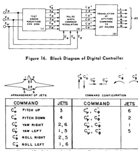
Since portions of the flight are outside the atmosphere in regions where the dynamic pressure is too small to make use of aerodynamic surfaces for control, a reaction jet system is required. Figures 16 and 17 show the block diagram of the digital controller, the jet

configurations, the sign conventions, and the combination of jets required to execute various commands. To make the reaction jet control easier, a pulse width modulation scheme is used which makes the moment proportional to the error signal. To prevent continuous pulsing of the jets even for small errors, a deadzone is built into the controller.

E.

TRANSl. ATION

Ea £RqOR TEST A'nITUDE OF

E", MAGNITUDe ANO SIGN COMMANDS TO (I) JET PULS£S

(3)

Figure 16. Block Diagram of Digital Controller

I I\. 2

~-+~

--+---5 6

ARRANGEMENT of JETS COMMAND CONFIGURATION

}

""

COMMAND JETS COMMAND JETS

C+

e PITCH UP 3 C~,

C;

6

C~ PITCH DOWN 4 C;, C; 2

C ..

tv YAW RIGHT 2,6 C;., C~ I

C-

.,

YAW LEFT 1,5 _{C;, C~} 5

C+

..

ROLL RIGHT 2,5

c-

_..

ROLL LEFT 1,6

Figure 17. Relationship Between Commands and Jets

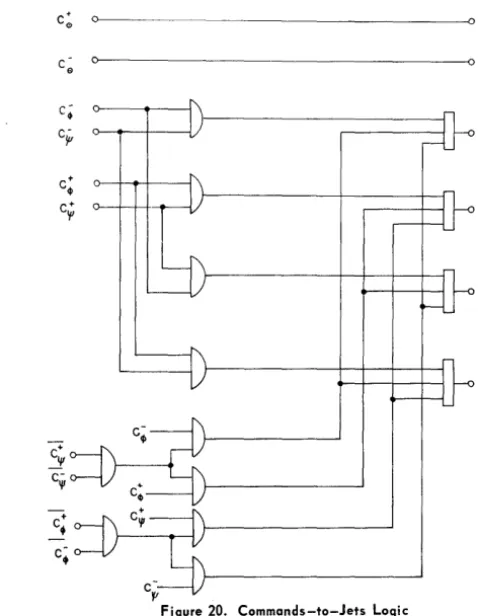
[image:10.620.59.523.61.330.2] [image:10.620.313.534.420.662.2]

modulation. Figure 20 shows the logic required to decode the commands so that the proper jets are used.

E;

-100

COMPo t - - - O

~--~---__ -~L

COMPo ~---4~--o

EMIN L

\00

Figure 18. Circuit for Testing Roll Error Magnitude and Sign

,. I ... -+100 IE I

v'

Figure 19. Pulse Width Command Modulation Circuit for Roll Angle

AND 2.!JIR-V

/3.f

AERODYNAMIC DYNAMIC AERO.FORCE FORCES PRESSURE COEFFICIENTS,

I

'-,DIY V

I

A:b

I

FORCE _o-.~ VELOCITY, 'IE LOCITY TRAHSFORMATI ON _HEADING

TRANSLATIONAL EQUATION S OF MOTI ON

V~

=

F~ + (~s Inn.) VN-(~CO 5 ..$\..)

r

Y.N

=

"*

+ 13"'-(~.sln..n.) VI -

4

y.

yo =

F,ri

-9" + COS.a)Ve +J1. y ...

c· _e 0 ~---~o 3

ee 0 _{---0 4}

C _~

e-If

c+ ~ c+

'I' 2

5

6

Commands-to-Jets Logic

The logic operations required in the simulation of the control system are performed on the DOS in parallel to all other operations in the digital section. The simulation of such a system by conventional analog techniques is a formidable

h

AND Z.3IR-V

OI..f HEAT

.--V.:.,.-_ ... TRANSFORMATION,

h TEMPERATURE

v

EQUATIONS

RANGES,

GUIDANCE

EQUATIONS

POSITION

CALCULATION

I

~

...il..-S-~&I _ ~

~

[image:11.620.286.525.48.356.2] [image:11.620.64.531.51.710.2] [image:11.620.79.532.418.691.2]

task (dozens of switches and relays would be required). The use of the 375 for such an operation would result in a significant increase

in digital computation time because of the large number of logic operations and the fast sampling rate required.

Digital Calculation on the 375: The digital program was written to make the digital calculation time as small as possible and to stay within a memory capacity of 4,000 words. The material which follows gives a description of the equations which are solved on the 375 and the details of the digital computer programm ing.

1. Summary of the Digital Calculations

Figure 21 shows the block diagram of the system of equations to be solved on the 375. A complete summary of the equations and symbols is given in Appendix A.

(Po

A B'C' : SPACE FIXED REFERENCE FRAME ABC: EARTH FI XED REFERENCE FRAME NED: LOCAL HORIZONTAL REFERENCE FRAME XVZ :BODY REFERENCE FRAME ,}..Or : SPHERICAL COORDINATES RELATIVE TO

[image:12.621.358.531.97.377.2] [image:12.621.314.534.100.692.2] [image:12.621.69.285.297.526.2] [image:12.621.315.530.444.681.2]

EARTH FIXED REFERENCE FRAME

Figure 22, Orientation of Space Fixed, Earth Fixed, and Body Reference Frames Used in Six Degrees of Freedom Simulation

The three -degree - of - freedom translational equations of motion are solved in a local horizontal coordinate system with axes along the north, east, and radial directions as shown in Figure 22. The gravity and altitude calculations are based upon an oblate model of the earth, and the U.S. Standard Atmosphere (1962) was stored in table form on the 375. Most of the equations are conventional and quite straightforward, with the exception of the heat transfer, temperature, and guidance equations which will be discussed in more detail.

The heat transfer and temperature equations are as follows:

2.70893

Iv

\2

qcs =

VR

yq~oi

qRS , = 144.9Rp ' 1.57

(v

- ~7

104

q = q' COS 1.50::: C cs

Ts

V

(3er

Ts=

4"

0-V+ -2-)

1 dp

(3 = (3 (h) = -

-E e p dh

The quantity (3 e is calculated from the stored density table by use of a second order curve fit technique to determine the derivative. These equations were calculated in the digital section because of the large numbers of complex functions required (i. e., Sine, COSine, log, exponential,

HEADING ERROR: cT'T - cr

square roots, etc.). However, they are easily computed on the 375 by use of library subroutines. Fortunately, these terms were also slow-varying, trajectory-dependent quantities so that the slower serial computation on the digital is acceptable. The temperature rate equations involving angular rates are calculated on the analog because of their rapidly varying characteristics.

Because of their critical accuracy requirements, the guidance calculations are also performed on the digital section. These can be separated into two parts: (1) the determination of the range-to-go (RTG) , heading angle to target (uT), cross range - to - go (CRTG), and heading error and, (2) the generation of down range and cross range errors (DRE and CRE) which are sent to the TRFCS and subsequently controlled to zero. The equations for range-to-go, heading angle, cross-range-to-go and heading error, which are determined from spherical trigonometric re-lations, are given in Appendix A. Figure 23 illustrates the physical significance of these quantitites. The down range and cross range errors used for guidance are generated as follows:

ATTITUDE INFO., AERODYNAMIC

FUNCTIONS

5

TRAJECTORY,4---t SENSOR

INFORMATION, OUTPUTS TO DISPLAYS

6

EVALUATE S I X ANALOG-DIGlTAL I _ _ ~ DI FF. EQUATIONS

-TRANSFER

"N' "0' vE,n.>...r,

GET INTEGR. CONST.

4

CR

E = CRTG - CRTGd RTG

d = fl (V) CRTG d = f

2(V)

The quantities f1 (V) and f2 (V) are the values of RTG and CRTG for a nominal re-entry. They are stored as a function of the relative velocity.

2. General Description of Digital Program

In addition to solving the translational, tempera-ture, and guidance equations, the digital program must accept mode control and timing commands from the DOS, scale variables as they are transferred in and out of the digital section, and finally, provide various input-output functions as described in the DOS section.

Figure 24 shows the flow diagram of the digital program. The executive program is discussed in detail in the section that follows. The dashed lines in the diagram link together the calculations which are performed when the IC mode of operation is

_ _ IC~O!.... __

OPERATE LOOP

2

PROGRAM

INITIALIZATION I - -

""1

9

RUNGE- KUTTA NUM.INTEGRATION, INTERMEDIATE a 1 - - - - ,

FINAL

CALCULATIONS

I

I

I

I

1

I

I

CALCULATION NO

OF HEAT TRANSFER YES RATES,TEMP.,AND _ _ _ _

VELOCITY, DYNAMIC PRESSURE.

">_ ... _-_--_--_--_-_--_--_--_-_---\ ANGULAR RATE t

I

.1

I

J

FLUX AT STAGNATION POINT

Figure 24. Flow Diagram of Digital Program

[image:13.620.74.535.349.703.2]

selected. All operations are performed except the Runge - Kutta integration shown in block 9. When the operate mode is selected, the integration loop is entered and three passes around the loop are made (see description of numerical integration which follows). At the end of three passes, the positions and velocities, temperatures and guidance functions are updated and the analog-to - digital and digital- analog-to - analog transfers are made. The executive loop is then re-entered and the cycle continued until a different mode is selected. The following section discusses this executive loop in detail.

3. Digital Executive Program

The main medium of communication through which the 375 receives the mode commands and timing from the DOS 350 is the digital executive program shown in Figure 25. This program is essentially a chain of test instructions through which the digital section interprets the DOS 350 commands and executes them by jumping to the respective portion of the stored program.

E/IIT

NO

YES

Figure 25. Digital Executive Program I

I

Since some of the symbols are not identified in the figure, a short explanation of the executive program follows. The first test determines whether T is greater than TF, where T is the current time (time elapsed since the beginning of this simulation run) and TF is final time indicating the end of the run. If final time is reached, results are outputed and the digital section is halted. When restarted, the digital program begins with the next decision. The next decision determines whether fast or slow time scaling is requested. If fast time scale is selected, the increment size for integration, DLT (delta t), becomes 1 sec; otherwise, it is 0.1 sec. The subsequent two test instructions simply switch the digital program into TIC or TYTI modes if so commanded by the mode control logic. (See Section B for a definition of these modes). The T > TT decision determines if it is time for the periodic dump of pre - selected digital parameters. The variable TT holds the time for the next dump, say 20, 30, 40, etc. seconds. TP is the printout time interval and increments TT when the dump time is reached.

If the dump switch is on and T > TT the output dump is performed; if not, the program proceeds to the next decision. The next test keeps the entire digital program under the timing control of the master timer. The 375 cannot proceed further until the next T1 pulse indicates the beginning of the next computational cycle. Further testing takes place only after the Tl pulse arrives. The TDA test enables the programmer to place the digital program into a loop where only DA transfer is performed. This mode serves as a convenient test for DA conversion. (This instruction may be removed from the program after the check-out phase is over). The last few tests are self-evident and require no explanation with the exception of the seemingly superfluous second test for dump. The test for dump in hold mode makes it possible to dump any time by putting the computer in hold mode prior to the dump request, in addition to or in lieu of periodic dumps. In this manner the programmer can determine parameter values with digital accuracy at any time during the simulation.

4. Numerical Integration

Unquestionably, one of the most complex and time-consuming parts of the digital program is the solution of the six simultaneous differential equations which provide the position (altitude, latitude, and longitude) and the velocity (radius rate, velocity east, velocity north) of the vehicle.

[image:14.618.70.292.343.688.2]

method. The basic method as ap'plied to a single differential equation is described briefly.

Let :

=

f(x,y) represent any first order equation

and

K4 = _hf(xn + h, Yn +

IS)

1

l1y ="6 (K 1 + 2K2 + 2K 3 + K₄)

Then, x 1 _n+

=

x hand y 1 = _{n+ n+} Y + _n 11 Y

The increment for the second interval is computed in a similar manner by means of the same formulae.

A computer flow diagram for this scheme is shown in Figure 26. The loop on the left side of this diagram corresponds to the constant calculations (kl, k2, k3, k4), while the loop on the right updates the independent variable and starts the calculation of the next increment. When the number of increments computed (n) is equal to the number desired (nf), the computation ends. Note that Xs and ys, the starting values for the current increment calculation, must not be destroyed during this process until the new starting values are produced since all formulae are dependent upon them.

Figure 26. Block Diagramof Numerical Integration (Fourth Order Runge.Kutta Method)

The preceding technique was extended to a system of six equations in an obvious manner.

While preparing the digital program an effort was made to combine the calculations due to the integration with other necessary calculations to minimize the processing time as well as the memory space requirements. This approach makes it difficult to trace the integration on the flow diagram of the digital program shown in Figure 24. For example, the Runge-Kutta constants are determined in block 6 and the variables are incremented for the calculation of

the next constant in block 9 (such as V E +

~1

... VE1etc., and the equations are evaluated with the increm entedvariables in blocks 3, 4, 6, and 7. The final calculation of the variables is performed in block 9.

The question may be asked by the competent reader: Why was this particular scheme chosen from many others available? In order to answer this question, the selection criteria are listed below.

(1) Self-starting method. It was desirable to choose a self - starting method to simplify programming andreduce mem-ory requirement. (If the method is not self-starting, another method is needed to calculate the first few points of the solution. This virtually doubles the integration program.)

(2) Accuracy. The error of the fourth order Runge-Kuttamethod is of the order of h5 and provides a wide enough range for h within which the accuracy of the calcula-tion is acceptable. (During the simUlacalcula-tion runs this reasoning proved to be a valid one.) The accuracy of calculation using the second or third order method was considered to be insufficient or marginal.

(3) Large time steps in integration. While proceSSing time associated with this method is conSiderable, the accuracy is good enough to allow larger time steps. The increase in computation time using Runge-Kutta is more than off set by the increase in allowable step size.

[image:15.621.72.289.78.272.2] [image:15.621.73.296.475.697.2]

simu-lation is frequently called upon to change time scale, thus requiring a different time step for the integration.

5. Utility Programs

In order to satisfy the various data handling needs (type in, type out, punch tape, convert binary to decimal, etc.), an excessive amount of digital programming must be done. Fortunately, all these programs are already available, tested, and clear ly desc.ribed in the 375' s "software package" . This is no small feat if one considers that the above programs, together with the numerous subroutines, normally add up to about 75

%

of all digital programming required. Furthermore, as it will be pointed out later, several program s are available to make the debugging and updating procedures efficient and fast.

Analog Section: The analog computer is the one

link of the HYDAC 2400 system ideally suited for control system simulation by virtue of its cap-ability for high speed and parallel computation, and its input! output flexibility. Output data can be displayed in a multitude of forms such as X- Y plots, strip chart plots, oscilloscope displays, auxiliary meters, etc. SpeCial purpose input equipm ent can be adapted easily for compatible operation with the analog computer.

1.. General Mechanization

The block diagram of Figure 27 delineates the mechanization of the analog program. A listing

FROM DOS 3:10 I AND 37:1

9-::r:

J _J

ATTITUDE I

---'.~-~IO< .A;G.L~ 1 4

-C,(cI,MI C.(o(,MI

I.;,J-<,M)

1·

L,D,Y

Je.¢

J AER~g~~~1C

J

I

EULER ANGlJ

J L,D, Y

l

0) ¢

J

Ip,Q,R

I ...

~

l

P,Q,R

J

AERODYNAMIC

I

I TORQUES L, M, N

AERO. MOMENTl L M N

I

COEFFICIENTS I ' ,

: t

bE' ba , bR

REACTION ~IET I

J

I SHORT PERIOD I

---,.T!,-s - + - - - 1 - , SENSOR t--_ol_,'-'-13 _ _ ---'

_Ts>--;..--_ _ _ ---tJ EQUATIONS 1

T, v, a,

I

COCKPIT

I

6. RTG, • AND DISPLAYS

CRTG,h. ORE, CRe

Figure 27. Block Diagram of Analog Section

I TO DOS 3:10 AND 37S

,

,<::>(. /3.,it

of the equations simulated in the analog section is given in Appendix A. The symbols used in the equations are defined in Appendix B.

As previously mentioned, the TRFCS and rotational dynamics were programmed on the analog due to their rapidly varying characteristics. When the vehicle is in the atmosphere, the vehicle attitude is controlled by aerodynamic control surfaces. The aerodynamic control moments are calculated from the surface deflections and the moment coefficients generated on the DOS 350. Out of the atmosphere, the vehicle attitude is controlled by areaction jet control system. The jet pulse logic is generated on the DOS 350 and transferred to the analog section where the moments are produced and fed into the angular acceleration equations. The angular rates, generated from the angular acceleration equations, are used to calculate the Euler angles Q and fJ. These angles are used to resolve gravity into the body axis for use in the ~: and ~ equations shown below.

g v2 _L

oc

= (J..- ~) (cos{}coscpcosoc+ sin{}sinoc)

-V ~ mV

+ Q - (Pcosoc+ Rsinoc).B

gr V,2 Y

~ == '1- rV (cos {} sin cp) y-Rcosoc+ Psinoc+ mV +

E.

.B - (gr -

.::f.

(cos

e

cos cp sin oc- sin {} cos oc) .B

.mV r

These seemingly redundant force equations, d; and

t3,

are computed on the analog since they are required in the short period sensor equations shown below. The aerodynamic force coefficients in the ~ and ~ equations are generated on the DOS 350. The geometric definitions of q; and .B are shown in Figure 28.

x

x~z - BODY AXES

Figure 28. Definition of oc and.B Angles

The short period sensor equations are:

• 2 •

T.== Ts(1- ~875.oc) - .375ococTs

[image:16.612.326.517.307.395.2] [image:16.612.50.282.409.687.2]

The quantity

T

is the temperature rate at the nose sensor; L1

T

is the temperature rate differential

between the two wing sensors (See Figure 1). The stagnation point temperature information, T s and

T

_{s , which is used in these sensor} equ~tions, i!3 calculated in the digital section. The T and ~ T are used in the TRFCS control equations shown below:

OR = f₂(L1'b + K₄0_a

Ilc = f₃Cf)

The

T

and L1

t

terms supply damping to the control equations, alleviating the heating problems associated with an undamped traj ectory. Closed loop guidance is achieved by adjusting the pitch axis controls with a compensated down range error, DRE, and adjusting the Ilc to compensate

for the cross range error, CRE. The pilot can control the range manually by adjusting his temperature rate profile to eliminate the displayed down range and cross range errors.

2. Cockpit Simulator and Display Equipment

A cockpit simulator is utilized to evaluate the TRFCS in the manual mode and is trunked directly to the analog computer. Computer outputs drive display meters on the TRFCS CONTROL P ANEL* which monitor the following parameters:

(1) temperatures (2) temperature rate (3) velocity

(4) acceleration (5) pitch damper (6) yaw damper (7) bank angle (8) heading angle (9) elevator trim (10) range

(11) range error (12) cross range (13) cross range error (14) altitude

*Refer to Figures 28 and 29 of Reference (1).

As seen in the analog program block diagram, many of these parameters are transferred from the digital section. Some of the parameters, though not necessary for control, indicate

tra-jectory status and, therefore, maintain the pilot's confidence in his control information. The above parameters and other pertinent data are recorded on strip charts and X- Y plots for permanent record of each flight.

Vehicle attitudes commanded by the flight control system are displayed on a large oscilloscope. An illustration of the display at various attitudes is shown in Figure 29.

ANGLE OF ATTACK = 0 BANK ANGLE-=O

ANGLE OF ATTACK =4So BANK ANGLE=O

ANGLE OF ATTACK==4So BANK ANGLE=30°

[image:17.613.326.535.214.598.2]

REFERENCES

(1) Stalony-Dobrzanski, J. "Temperature Rate Flight Control System," Lecture given at University of California, Los Angeles, August 1963 (2) Stalony-Dobrzanski, J. "Application of Temperature Rate to Manual Flight Control of Re-entry Vehicles and Energy Management, "Proceedings

National Aerospace Electronics Conference," Dayton, Ohio, 1962

(3) Chapman, Dean R. "An Ana Iys is of the Corridor and Guidance Requirements for Supercircular Entry Into Planetary Atmosphere," NASA TR R -55, 1959

(4) Frederickson, A. A • "Ana log Computer Mechanization for Gu idance Law Stud ies," The Boeing Company, Report #02-8117, November 1960 (5) Lees, Lester, Hartwig, F. W., and Cohen, C. B. "Use of Aerodynamic Lift During Entry Into the Earth's Atmosphere," Jet Propulsion, Vol. 29,

No.9, September 1959, p. 633

APPENDIX A

I. Digital Computer Equations

A. Basic Translational Equations in Local Horizontal System

The translational equations are solved in a local horizontal coordinate system with axes along the north, east, and radial directions. Figure 23 shows this coordinate system.

.• Fr . }

r = - - g r + ( ( c o s O v_{E +OV N} (1)

m

. F E ' ' .

V E = - + «( sin n) _{VN -} «( cos

m

r (3)

m

B. Aerodynamic Force Calculation and Transformation

The aerodynamic forces are calculated wi th respect to the relative velocity. vector (lift, drag, and y axis acceleration) and then transformed into the local horizontal coordinate system.

D gSC_o

Fr L Y D

=(-cosfJ.--sinfJ.) costl"--sin)

m m m m

F L Y L Y

~ = - ( -sinfJ. +-cosfJ.) cosa-·[(-cosfJ. - - sinfJ.) sin I

m m m m m

+ Ecos Y] sina

m

FE L Y L Y

- = ( -sinfJ. +-cosfJ.) sina - [(-cosfJ. - -sinfJ.) sin¥'

m m m m m

+ ~ cosY) cosa

m

C. Angular Rate and Position Calculation

(4)

(5)

(7)

(8)

The derivatives of the space fixed coordinates, P. and ~ , are solved as functions of the inertial velocities, V_N and VEe The derivative of the longitude is calculated by subtracting the earth's rotational rate from ~. Since the earth rotates in the longitudinal direction,

n

is the latitude. Altitude is calculated with respect to an oblate earth.

. vN

0=-,- (10)

r

. V_E

(= rcosO

,\ = ~-Wo

(11)

( 12)

(13)

D. Velocity, Velocity Heading and Flight Path Angle Calculations

The total relative (to the earth) velocity is calculated from the velocity components in the N, E and radial directions. The horizontal relative velocity has two components, east and north. The easterly relative velocity is the difference between VE and the tangential rate of the earths rotation. The relative northerly velocity is the same as the northerly inertial velocity. The flight path angle, d, is the angle between the horizontal and the total velocity vectors. The velocity heading angle, u , is measured from east to north.

v =

J

v2 + v2 + i: 2 ( 14)

ER NR

VH =

J

V_E2_R + V_N2_R (15)

V E R = V E - rwo cos 0 ( 16)

sinJ'=i.

V (17)

VH

cosi' ='1 ( 18)

¥= tan -1 r ( 19)

VH

VN ₍₂₀₎

sina = -VH

cosa = VE R ₍₂₁₎

VH

VN

a = tan-1- -_V (22)

ER

E. DenSity and Dynamic Pressure

The density is tabulated in square root form to com-press the range of variation and was taken from U.S. Standard Atmosphere (1962). The dynamic pressure is a function of density and velocity.

g = (~_ Vp V)2

V2

F. Gravity Calculation

(23)

(24)

The gravity components are calculated for an oblate-spheroid-shaped earth. Since the earth is assumed to be rotationally symmetrical, gE = O.

GM 3Jr E2 1 2

g R = - - [ l + - - (--sin 0»)

r2 r2 3 (25)

2GMJr ~

gN = - - r -_{4 -} sin 0 cos 0 (26)

G. Heat Transfer and Temperature Equations

gcS=---vg- -. 2.70893

(V

~

VR 10"

~ '17

gR S = 144.9Rp 1 .57

\1~J

gc = g c S GOs 1. Sex

g g cos 6 ex

R = R S

TS V (3 .. ~ Ts =4'C3-y+ 2)

gT S = {(iRS + gc s) dt (3 = ~ dp

e p dn

H. Target Heading Angle, Range-to-go and

Cross Range-to-go

(27)

(28)

(29)

(30)

(31)

(32)

(33)

(34)

(35)

The range and heading angles are calculated using spherical trigonometry and the resulting angles are multiplied by the earth radius yielding the range.

cosU tanU T - sin 0 cos (AT- A) tan aT = sin(A

T- A)

sin (A -A)

sin (AT - A) tan 8 = .

RTG _{cosaT[tanO T SlOO + cosO cos (AT-A)}

RTG = (e_{RTG) fE}

tanCR = - tan (aT - a) _{sin 8RTG}

CRTG = _{(CR)r E}

I. Heading Error

The angle between the great circle heading to the target, (T T' and the velocity heading, (T.

(36)

(37)

(38)

Heading Error

=

(T T - (T (39)

J. Guidance Equations

Error equations for use in the TRFCS

DRE = RTG - RTG_d RTG_d = £1 (V)

CR E = CRTG - CRTGd

CRTG_d =

9

V)

(40)

(41)

II. Analog Computer Equations

A. Angular Acceleration

The following equations are calculated in the body system:

. ~IZ-IY~ L+Mx

P= Q R +

-Ix I x

. t

ly

- Ix) N + Mz

R = - - - -P Q +

-I_z I_z

B. Aerodynamic Torques

(42)

(43)

(44)

These parameters are generated by the moment of aerodynamic forces.

C. Euler Angles

Gener ated for local horizontal to body axis transformation.

8 = f (Q cos cp - R sin cp) dt

cp = J(p + tan 8 (Q sin cp + R cos cp)] dt

D. Attitude Rate Equations

Generated in this form for use in the heat sensor equations.

~ = (gr - Vl2.\cos 8 cos cpcosa + sin 8 sinoc) -~

~V ~f mY

+ Q - (Pcos a + R sin oc)(3

~

=

~

-

~r~COS8

sincp) - R cosoc +P sinoc+ :Y

(45)

(46)

(48)

(49)

(50)

2 (51)

+...!2. (3 - (g -~ (cos8coscpsinoc- sin8cosoc) (3 mY r f

~ = P cos ex + QB + R sin ex E. Heat Sensor Equations

These short period equations are used for control and are discussed in the text.

• • 2 •

T = Ts (1 - .1875oc ) - .375 oc oc Ts

~ T = .021T s(3

(52)

(53)

F. TRFCS Control Equations

The control parameters include the variable surfaces and the commanded bank angle.

(56)

(57)

(58)

Variable V N V E r F N m F -s m F r m g r gN L m D m y m V N V E VI V V H V NR V ER M n

e

A {J p APPENDIX B

DE FINITION OF SYMBOLS

Definition Variable

acceleration north (local level R

coordinates)

p

acceleration east (local level

Q coordinates)

R acceleration up (local level coordinates)

()

}

¢ aerodynamic acceleration north

L

aerodynamic acceleration east

M

aerodynamic acceleration up

N

gravitational acceleration up M

x

gravitational acceleration north M Y

M

z

lift acceleration _n

A

drag acceleration

side force acceleration {J

f.L

velocity north, inertial ¢

velocity east, inertial ()

radius rate t/J

f.L total inertial velocity

0

total relative velocity E

0

relative horizontal velocity a

0

velocity north, relative (equals V N)

r

velocity east, relative

a

mach number aT

latitude rate p

longitude rate, inertial

longitude rate, relative

h rate of change of angle of attack

DRE rate of change of angle of side slip

roll angular acceleration CR

E

Definition

yaw angular acceleration

roll rate about the body x-axis

pitch rate about the body y-axis

yaw rate about the body z-axis

Euler rates of body axis with respect to local horizontal

aerodynamic torque about the body x axis

aerodynamic torque about the body yaxis

aerodynamic torque about the body z axis

reaction jet moment about the body x'axis

reaction jet moment about the body yaxis

reaction jet moment about the body z axis

latitude

longitude

angle of attack

angle of side slip

bank angle (lift vector with vertical plane)

body roll angle

body pitch angle

body heading angle

bank angular rate

elevator deflection angle

aileron deflection angle

rudder deflection angle

flight path angle (+ for

r

+)

velocity heading angle (to the north from east)

heading to target (+ to the north from east)

air density

radial distance from earth center to

vehicle

altitude

down range error

Variable Definition Variable Definition

CRTG cross-range-to-go T temperature at sensor

C side force coefficient T temperature at stagnation point

y s

~T differential temperature rate

q dynamic pressure

between wing sensors

C lift coefficient _{GM earth gravitational constant}

L

C ₀ drag coefficient earth oblateness factor

C pitching moment coefficient radius of the earth-equatorial

M

C1(3 rolling moment coefficient due to

eccentricity of the earth

side slip _CU

o rotation rate of the earth

Cry (3 yawing moment coefficient due to

side slip _emissivity

Co

rolling moment coefficient due to

a _{aileron deflection} a

B Stefan Boltzman constant

C." yawing moment coefficient due to g _{sea level gravity}

°a _{aileron deflection} 0

~o yawing moment coefficient due to

m mass of the vehicle

r rudder deflection

C

lo rolling moment coefficient due to

r rudder deflection s wing area

q _{radiative heat transfer rate at}

rs _{b wing span}

stagnation point

qc s convective heat transfer rate at _{wing chord}

stagnation point c

qr radiative heat transfer rate at sensor I _{moment of inertia about x axis}

location x

qc convective heat transfer rate at sensor I moment of inertia about y axis

location

y

qTs total integrated heat flux at stagnation I z moment of inertial about z axis

point

T temperature rate at sensor location R nose cap radius

T temperature rate at stagnation point (3e exponential index of the atmosphere