THE IMPACT OF LOCATION BASED ATTACKS ON GEOGRAPHICAL ROUTING PROTOCOLS

REAL CODED GENETIC ALGORITHM (RCGA): A NEW

RCGA MUTATOR CALLED SCALE TRUNCATED PARETO

MUTATION

*1

SIEW MOOI LIM, 2MD. NASIR SULAIMAN, 3ABU BAKAR MD. SULTAN, 4NORWATI MUSTAPHA, 5BIMO ARIO TEJO

1,2,3,4

Faculty Of Computer Science And Information Technology, Universiti Putra Malaysia, Malaysia

5 _{Centre For Infectious Diseases Research, Surya University, Indonesia}

E-mail: *[email protected], [email protected] , [email protected] , 4

[email protected], [email protected]

* Corresponding author

ABSTRACT

This paper presents a comparison in the performance analysis between a newly developed mutation operator called Scaled Truncated Pareto Mutation (STPM) and an existing mutation operator called Log Logistic Mutation (LLM). STPM is used with Laplace Crossover (LX) taken from literature to form a new generational RCGA called LX-STPM. The performance of LX-STPM is compared with an existing RCGA called LX-LLM on a set of 10 benchmark global optimization test problems based on a few performance criterions to investigate the reliability, efficiency, accuracy and quality of solutions of both optimization algorithms. The final outcomes show that LX-STPM is far superior than LX-LLM at all aspects.

Keywords: Real Coded Genetic Algorithms, Mutation Operator, Crossover Operator, Global Optimization

1. INTRODUCTION

In light of continuous optimization, the variables applied in the objective function can assume real numbers, as opposed to discrete or combinatorial optimization, in which the variables may be binary or integer. As such, continuous optimizations are compartmented into several paradigms with certain assumptions differing in the objective function, variables and constraints. In fact, many real life problems are modeled as continuous nonlinear optimization problems and this study seeks to find the optimal solution to these problems.

A global optimization problem is defined as:

given f : ℜn _→ℜ a continuous function and S ⊂ℜn, find its global minimum f* = min { f (x): x _∈ S} and the set X* of all global minimizers X*(f) = {x* ∈ S: f(x*) = f*} [1].

Global optimization algorithms are mainly categorized into deterministic and stochastic

approaches. A few common unconstrained deterministic techniques are like Simplex Method, Newton's Method, Quasi-Newton Methods and Conjugate Direction Methods. These techniques employ a rigid mathematical tabulation with no irregular elements. Said algorithms primarily use linear algebra to compute the gradient and Hessian of the response variables. Most importantly, they ensure a theoretical guarantee of finding the global minimum if not the local minimum whose objective function value differs by at worst ℰ from the global one for a given ℰ > 0.

Commonly used stochastic algorithms include

Simulated Annealing, Particle Swarm

tracking a global optimum, capable of performing

on single and multi-objective optimization

problems, and it is more well-suited to black-box formulations and glitchfunctions [2].

Evolutionary algorithms (EAs) involve the

investigation of associated fields such as

developmental biology population ecology, co-evolutionary biology and population genetics. Many resources have been published on the theory of evolution including Darwin [3], Huxley [4] and Futuyma [5]. Scientific book publications such as Dennett [6] and Dawkins [7] are also available. Other seminal work by Koza [8] and Schwefel [9] deliberate on genetic programming and evolution strategies respectively.

Fogel [10] offers a comprehensive review of the history of research into the use of simulated evolutionary processes for problem solving. Two volumes of "Evolutionary Computation" by Bӓck, Fogel and Michalewics [11, 12] covers the major techniques, theory and application of the processes. Prominent authors such as De Jong [13], Fogel [10] and Eiben and Smith [14] are responsible for modern books on the unified field of Evolutionary Computation and Evolutionary Algorithms.

Evolutionary algorithms (EA) consist of three population based heuristic methodologies which are

genetic algorithms (GA), evolutionary

programming and evolutionary strategies. GA is a programming method brought forth by Holland in the 1960s [15]. GA is a group of biologically motivated optimizations techniques that evolve a population of individuals who would thrive in the survival of the fittest going into the next generation. The central operations of GA are reproduction, crossover and mutation on populations. The crossover operator takes two genotypes and combines them to form a new one either by merging or by exchanging the values of the genes. The mutation operator modifies one or multiple genes. In short, GA works in three (3) steps:

i) Form the problem and encode them into a set of binary strings;

ii) Create a new population through reproduction and mating processes;

iii) Evaluate the fitness and select the new generation.

The traditional and most common

representation in GAs is binary encodings which they can be easily manipulated by reproduction

operators to almost any desired representation. However, there persist several drawbacks of binary genetic representations [16]. Binary coded GAs (BCGA) are not proper for GAs searches and they are not able to assure that using GAs to solve problems of bounded complexity would be reliable and predictable [17]. Furthermore, BCGA was found to perform more effectively only on small and moderate size problems which detail precision in the solution are not critical. BCGA may

encounter certain intricacies dealing with

continuous search space. One difficulty which arises is the Hamming cliffs associated with certain strings, from which a transition to a neighboring solution (in real space) requires alteration of many bits. Gray code can alleviate the Hamming cliff problem but it needs huge computations [18].

The limitations of binary encoding are the main reasons for developing algorithms using real encoding of chromosomes representations. GAs

which make use of real number vector

representation of chromosomes are termed as Real Coded GA (RCGA). RCGA is used in a lot of applications and is recommended for optimization problems where the parameter space is continuous [19].

Prior works on RCGA have been found to be some specific applications, such as for chemometric problems, for the use of metaoperators to find the most adequate parameters for a standard GA, for numerical optimization on constant domains, etc [19,20, 21, 22]. A review related to RCGA is presented in [23]. Researches of RCGA in recent years for function optimization have proven to

outperform traditional bit string based

representation [23, 24].

Many RCGA researchers are shifting their

attention towards designing new crossover

operators to improve the performance of function optimization [25]. There has also been studies conducted on the varieties of mutation techniques to improve the GAs performance [26].

The paper is presented as such:

Section 2 presents literature review on real coded mutation operators.

Section 3 describes the proposed STPM and other operators used in this study

Section 7 includes discussions and explanation of results.

Section 8 reaffirms previous notions with a conclusion.

2. LITERATURE REVIEW ON MUTATION OPERATORS

Mutation operation functions to alter the offspring genes. A mutator will escalate the diversity of the population and this inadvertently allow GAs to explore and exploit the search space [27]. Literature reviews on mutation operations reported in [28, 29] encompasses random (uniform) mutation, non-uniform mutation, breeder GA mutation, boundary mutation, continuous modal mutation, Gaussian mutation, pointed directed mutation, discrete modal mutation, principal component analysis mutation, polynomial mutation operator, Makinen, Periaux and Toivanen mutation and wavelet mutation. Albayrak and Allahverdi [30] came up with a Greedy Sub Tour Mutation (GSTM) which employs classical and greedy techniques to find the shortest distance in the traveling salesman dilemma.

Several other forms of mutating operators found in the literature include mirror mutation, percentage mutation, edge mutation and tension vector mutation. The operation of mirror mutation and the binary bit-flipping mutation are similar. The percentage mutation replaces a gene with a random percentage of its value within the interval [80%, 120%]. The edge mutation and the tension vector mutation are based on the breadth-first (BF)

force-based and tension vector methods

respectively [31].

3. THE PROPOSED SCALED TRUNCATED PARETO MUTATION (STPM) AND OTHER OPERATORS USED IN THIS STUDY

3.1 STPM

A Scaled Truncated Pareto Mutation operator is proposed. This operator is built based on the formula to generate Pareto random variables. The truncated Pareto distribution has three parameters α, L and H. α determines the shape, L denotes the lower bound, and H denotes the higher (upper) bound of the evaluation function to be optimised.

The probability density function is:

1

where, , 0.

Applying inverse transformation, the equation for U as uniformly distributed function is defined as:

1

1

Also, is truncated Pareto distributed as:

||

_ഀభ

A modulus, | | is used to eliminate the possible imaginary number produce by the algorithm. To apply the Truncated Pareto Distribution as the

mutation operator, an adjustable scale, is

introduced. is added to make sure that is not over-weighted. If is over-weighted, there will be a chance of good chromosomes being alter in the process. Thus, the newly mutated offspring m is defined as:

|| ,

,

where P is the parent, and / ,

to determine the direction of the mutation. By experiment, and α are best kept at 10 and 3 respectively. Hence this mutation operator is known as Scaled Truncated Pareto Mutation.

3.2. Laplace Crossover (LX)

Deep and Thakur [25] advocated a new parent centric real coded crossover operator, so named the Laplace crossover (LX) as described below:

In LX, two offsprings C1 and C2 are generated from

a pair of parents K1 and K2 obtained after selection:

Generate a random number, ∈ _[0,1],

if ≤ 0.5;

then C1 = K1 + βх d

C2 = K2 + βх d

then C1 = K1 - βх d

C2 = K2 - βх d

3.3. Log Logistic Mutation (LLM)

Deep Kusum et al [32] suggested a distribution mutation according to Log Logistic distribution. A mutated solution, S is created in the area near the solution Z as follows:

Generate a random number, ∈ [0,1],

if < T;

then S = Z - λ (Z - L)

else if ≥ T;

then S = Z + λ (U - Z)

Where λ is a random number following Log

Logistic distribution, T =

, L and U are the

lower and upper bounds of decision variable.

4. THE PROPOSED NEW RCGAS

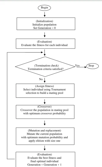
The objective of the present study is to introduce a newly designed mutation operator, STPM. STPM will make use of an existing crossover found in the literature namely LX to form a new RCGA namely LX-STPM. The performance of LX-STPM will be evaluated and compared with another RCGA from literature namely LX-LLM. Both of the RCGAs employ the same crossover, LX; therefore, a fair and unbiased comparison of performance between the two mutators can be made. Figure 1 shows the flow chart of both RCGAs used in this comparative study.

5. TEN (10) BENCHMARKING FUNCTIONS

This section presents 10 diverse and unbiased chosen set of standard benchmark functions which are used to examine the performance analysis of LX-STPM and LX-LLM. These functions have diverse properties in terms of complexity and modality. The dimension, problem domain size and optimal solution are denoted by D, L ≤ xi ≤ U and

f(x*) = f(x1, x2, x3...xn) respectively. L and U

represent the lower and upper bound of the variables. Function no. 1 to 5 are nonscalable and function no. 6 to 10 are scalable. That said, in a scalable function, the number of decision variables can be increased or decreased as per users desired. The number of variables for all the scalable benchmarking functions is fixed at 30. A

multimodal function has many local optima, but

only one global optimum. When the

dimensionality of a problem increases, the search space will increase exponentially to the difficulty of a problem. As such, the potential for separation is a gauge of the difficulty of benchmark functions. The properties involved in such processes to determine the optimization level is elaborated in [33].

5.1. The Formulas And Features Of The Five (5) Nonscalable Functions Are Given Below:

1. Easom 2D (Unimodal)

The global minimum has a small area relative to the search space.

Min f (x) = -cos(x1)cos(x2)exp(-(x1-π)2-( x2-π)2)

subject to -10 ≤ x1,x2 ≤ 10. The global minimum is

located at x* = f (π, π) and f (x*) = -1

2. Becker and Lago (Unimodal)

Min f (x) = (|x1| - 5)2 + (|x2| - 5)2

subject to -10 ≤ x1, x2 ≤ 10. The function has four

minima located at x* = f (±5, ±5), all with f (x*) = 0

3. Bohachevsky 1 (Continuous, differentiable, separable, non-scalable, multimodal)

Min f (x) = x1 2

+ 2x2 2

- 0.3cos(3πx₁) - 0.4cos(4πx₂) + 0.7

subject to -50 ≤ x1, x2 ≤ 50. The global minimum is

located at x* = f (0, 0) and f (x*) = 0

4. Eggcrate (Continuous, separable, non-scalable)

Min f (x) = x12 + x22 + 25(sin2x1 + sin2x2)

subject to -2π≤ x1, x2 ≤ 2π. The global minimum is

located at x* = f (0, 0) and f (x*) = 0

5. Periodic (Separable)

Min f (x) = 1 + sin2x1 + sin2x2 - 0.1exp(-x12 - x22)

subject to -10 ≤ x1, x2 ≤ 10. The global minimum is

5.2 The Formulas And Features Of Five (5) Scalable Functions Are Given Below:

6. Sphere (Continuous, differentiable, separable, scalable, multimodal. This function is easily converge to the global optimum)

Min x

n

i=1

subject to -5.12 ≤ xi ≤ 5.12. The global minimum is located at x* = f (0, 0, ..., 0) and f (x*) = 0

7. Rosenbrock (Continuous, differentiable, non-separable, scalable, unimodal)

Min x 100

1

n-1

i=1

subject to -30 ≤ x1 ≤ 30. The global minimum is

located at x* = f (1, 1, 1, ..., 1) and f (x*) = 0

8. Rastrigin (Non-linear multimodal. This function is fairly difficult due to the large search space and large number of local minima.)

Min x 10n ! " 10cos 2'(

n

i=1

subject to -5.12 ≤ xi ≤ 5.12, i = 1, ..., n. The global minimum is located at x* = f (0, 0, ... , 0) and f (x*) = 0

9. Schewefel problem 3 (Continuous, differentiable, non-separable, scalable, unimodal)

Min x || ! )

n

i=1

subject to -10 ≤ x1 ≤ 10. The global minimum is

located at x* = f (0, 0, ... , 0) and f (x*) = 0

10. Griewank (Continuous, differentiable, non- separable, scalable, multimodal)

Min x 1 !₄₀₀₀ 1 ) cos +

x √i-

n

i=1

subject to -600 ≤ xi ≤ 600. The global minimum is located at x* = f (0, 0, ..., 0) and f (x*) = 0

6. EXPERIMENTAL SETUP

The primary setback of GA is its several tuning variables which require proper setting. GAs major control parameters and operations which have significant impact on GA's solution quality includes population size, number of generations, crossover and mutation rates [34]. Both of the algorithms used tournament selection and both algorithms are elite preserving with elitism size one. Elitism prevents losing the best found solution so it can very rapidly increase performance of GA. A heavy

experimentation study of various possible

combinations of crossover probability, mutation rate and tournament size were carried out to determine the optimal parameter setting for both of the RCGAs.

The termination principles and populations size were taken from [32]. The termination principles depends on either an optimum solution found by the algorithm lies within the specified accuracy (0.01) of known optimum or the predetermined maximum number of generations (3,000) is reached, or whichever occurs earlier. Population size is assumed as ten (10) times the number of variables. Each GA has been run 100 times using same initial populations; each run is initiated using a different set of initial population.

Table 1 shows the final parameter settings; Pc,

Pm and Ts represent crossover and mutation rate and

tournament size respectively. We recommend these parameter settings for the present study based on the positive results obtained for majority problems. However, these parameters may not be suitable for other problems in general. According to [35] there has been no generalconclusion drawn in relation to the optimum parameterization of operators. Both of the algorithms are implemented in MATLAB 2012 and the experiments are done on a Core i5 Processor with 2.40GHz speed and 4.00GB RAM under Windows 7 platform.

7. RESULTS AND DISCUSSIONS

minimum, or at least approaching it sufficiently closely. All the performance evaluation criteria are calculated based on success run only and they are logged for each algorithm and benchmark function.

When f (x)FoundOpt - f (x)KnownOpt ≤ 0.01, it is defined

as a success run, where f(x)FoundOpt is the optimum

value found when the algorithm terminates and

f(x)KnownOpt is the known global minimum of the

problem.

Success rate (SR) = ! "##""$ "

!%&$ ! " x 100

Average error (AE) = ∑ ೙ ಷ೚ೠ೙೏ೀ೛೟ ಼೙೚ೢ೙ೀ೛೟

where, n is the total number of runs.

Average number of function evaluations (AFE).

Table 2 shows the results of AFE and SR of all

the ten (10) problems for both of the algorithms. It is observed that both algorithms are able to solve all the ten (10) problems. LX-STPM requires less function evaluation except function no 3. Both algorithms achieved 100% success rate for seven (7) of the problems (function no. 1, 2, 3, 4, 6, 8, 10). For the remaining three (3) problems (function no. 5, 7 and 9), LX-STPM achieved higher success rate. In 9 out of 10 problems, LX-STPM totally outperforms LX-LLM on both of the criterions. It proved that LX-STPM to be a more reliable and efficient algorithm.

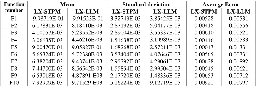
Table 3 shows the results of mean, standard

deviation and AE of all the ten (10) problems for both algorithms. Mean and standard deviation of the objective functions are to compare the quality of the solutions found. All the mean objective function values and the corresponding standard deviations achieved by LX-STPM are lower than LLM except function no 9. Furthermore, LX-STPM produced lower average error for all the problems, except function no. 3. In 8 out of 10 problems, LX-STPM totally outperforms LX-LLM on all three criterions. It proved that LX-STPM to be a more accurate algorithm.

8. CONCLUSIONS

In this paper, a real coded mutation operator called Scale Truncated Pareto Mutation (STPM) is proposed. This operator is implemented based on the formula to generate Pareto random variables. The performance of STPM is compared with an existing real coded mutation called Log Logistic

Mutation (LLM). In order to have a fair comparison, both of the mutating operators made use of the same crossover called Laplace Crossover (LX) adapted from the literature. The performance of the two real coded genetic algorithms (RCGAs) which are LX-STPM and LX-LLM are tested on a set of 10 benchmark global optimization test problems. Optimal parameters were set up for both of the RCGAs to run the experiments. Numerical results presented in Table 2 shows that LX-STPM outperformed LX-LLM in all aspects and proved its reliability (robustness) and efficiency through the evaluation performance of success rate (SR) and average number of function evaluations (AFE) respectively. In the same light, numerical results in

Table 3 shows that STPM outperforms

LX-LLM in all aspects and proved its accuracy through the evaluation performance of average error, mean of objective function and its corresponding standard deviation.

REFERENCES

[1] Lavor C, Maculan N. A function to test methods applied to global minimization of potential energy of molecules. Numerical Algorithms 2004; 35: 287-300

[2] Liberti L, Kucherenko S. Comparison of deterministic and stochastic approaches to global optimization. International Transactions in Operational Research 2005; 12: 263-285

[3] Darwin C, Bynum WF. The origin of species by means of natural selection: or, the preservation of favored races in the struggle for life: AL Burt. 2009

[4] Huxley J. Evolution. The Modern Synthesis. Evolution.The Modern Synthesis. 1942

[5] D. Futuyma. Evolution: Sinauer Associates Inc. 2009

[6] Dennett D. Darwin’s Dangerous Idea Simon & Schuster. New York 1995

[7] Dawkins R. The selfish gene: Oxford university press. 2006

[8] Koza JR. Genetic Programming: On the programming of computers by means of natural selection: MIT press. 1992

[9] Schwefel H. Numerical optimization of

computer models: John Wiley & Sons, Inc. 1981 [10] Fogel DB. Evolutionary computation: toward

a new philosophy of machine intelligence: Wiley-IEEE Press. 2006

[11] T. Back, D. B. Fogel and Z. Michalewics, editors. Evolutionary Computation 1: Basic Algorithms and Operator: IoP. 2000

[12] T. Back, D. B. Fogel and Z. Michalewics, e

Advanced Algorithms and Operations: IoP. 2000

[13] De Jong KA. Genetic Algorithms are NOT Function Optimizers. 1992: 5-17

[14] Eiben AE, Smith JE. Introduction to evolutionary computing: Springer Berlin. 2010

[15] Holland JH. Adaption in Natural and Artificial Systems: University of Michigan press. 1975

[16] J. Antonisse. A new interpretation of schema notation that overturns the binary encoding constraint, in J.David Schaffer (Ed.) 1989, pp. 86-91

[17] Liang Y, Leung K, Xu Z. A novel splicing/decomposable binary encoding and its operators for genetic and evolutionary

algorithms.. Applied mathematics and

computation 2007; 190: 887-904

[18] Jin J, Yang X, Ding J. An improved simple

genetic algorithm—accelerating genetic

algorithm. Theory and Practice of System Engineering 2001; 4: 8-13

[19] Z. Michalewicz. Genetic algorithms + data structures = evolution programs: Springer. 1996

[20] Lucasius CB, Kateman G. Application of genetic algorithms in chemometrics 1989: 170-176

[21] Davis L. Adapting operator probabilities in genetic algorithms 1989: 61-69

[22] Wright AH. Genetic Algorithms for Real Parameter Qptimization, in: G.J.E. Rawlins (Ed.). Foundations of Genetic algorithms I, 1990: 205-218

[23]Herrera F, Lozano M, Verdegay JL. Tackling real-coded genetic algorithms: Operators and tools for behavioural analysis. Artificial Intelligence Review 1998; 12: 265-319

[24] Ono I, Satoh H, Kobayashi S. A real-coded genetic algorithm for function optimization using the unimodal normal distribution crossover. Transactions of the Japanese Society for Artificial Intelligence 1999; 14: 1146-1155 [25] Deep K, Thakur M. A new crossover operator for real coded genetic algorithms. Applied Mathematics and Computation 2007; 188: 895-911

[26] Tang P, Tseng M. Adaptive directed mutation for real-coded genetic algorithms. Applied Soft Computing 2012

[27] I. Korejo, S.Yang, C. Li. A directed mutation operator for real coded genetic algorithms, in:

C. Di Chio, et al. (Eds.). Evo Applications, Part I, LNCS 6024 2010: 491-500

[28] Deep K, Thakur M. A new mutation operator for real coded genetic algorithms. Applied mathematics and Computation 2007; 193: 230

[29] D.K. Pratihar. . Soft Computing, Alpha Science Internatioanl Ltd., Oxford, UK 2008 [30] Albayrak M, Allahverdi N. Development a

new mutation operator to solve the Traveling Salesman Problem by aid of Genetic

Algorithms. Expert Systems with Applications 2011; 38: 1313-1320

[31] Vrajitoru D, DeBoni J. Hybrid real-coded mutation for genetic algorithms applied to graph layouts 2005: 1563-1564

[32] Deep K, Katiyar V. A new real coded genetic algorithm operator: log logistic mutation 2012: 193-200

[33] Jamil M, Yang X. A literature survey of benchmark functions for global optimisation

problems. International Journal of

Mathematical Modelling and Numerical Optimisation 2013; 4: 150-194

Begin

(Initialization) Initialize population

Set Generation = 0

(Evaluation)

Evaluate the fitness for each individual

(Termination check) Yes Stop Termination criteria satisfied?

No

(Assign fitness)

Select individual using Tournament selection to build a mating pool

(Crossover)

Crossover the population in mating pool with optimum crossover probability

(Mutation and replacement) Mutate the current population with optimum mutation probability and

apply elitism with size one

(Evaluation) Evaluate the best fitness and

final optimal individual Generation = Generation + 1

Table 1: Parameter Setting For LX-STPM And LX-LLM

GA name Nonscalable Scalable

Pc Pm Ts Pc Pm Ts

LX-STPM 0.65 0.02 3 0.7 0.003 5

LX-LLM 0.70 0.02 3 0.65 0.003 4

Table 2: Computational Results Of Average Function Evaluation And Success Rate For All Ten (10) Problems

Function number

Average Function Evaluation Success Rate

LX-STPM LX-LLM LX-STPM LX-LLM

F1 129 325 100 100

F2 183 282 100 100

F3 636 528 100 100

F4 249 452 100 100

F5 103 883 80 64

F6 29,036 35,357 100 100

F7 152,254 183,475 85 72

F8 111,848 170,659 100 100

F9 40,573 50,598 95 86

F10 60,392 85,923 100 100

Table 3: Computational Results Of Mean Of Objective Function And Its Corresponding Standard Deviation And Average Error For All Ten (10) Problems.

Function number

Mean Standard deviation Average Error

LX-STPM LX-LLM LX-STPM LX-LLM LX-STPM LX-LLM

F1 -9.98719E-01 -9.91523E-01 3.32749E-03 3.85425E-03 0.00528 0.00531

F2 6.17831E-03 8.18410E-03 2.87192E-03 5.04177E-03 0.00418 0.00556

F3 4.10057E-03 5.23552E-03 2.89004E-03 3.55337E-03 0.00610 0.00521

F4 3.06635E-03 4.46216E-03 1.51638E-03 3.19989E-03 0.00446 0.00583

F5 9.00470E-01 9.05827E-01 1.68268E-03 2.57211E-03 0.00047 0.01331

F6 5.65324E-03 5.72380E-03 3.53404E-03 4.07646E-03 0.00565 0.00731

F7 6.38204E-03 9.43741E-03 2.95392E-03 4.29061E-03 0.00638 0.01892

F8 7.44700E-03 8.56542E-03 1.55854E-03 2.99504E-03 0.00545 0.00621

F9 6.53018E-03 4.87891-E03 2.17720E-03 1.48336E-03 0.00653 0.00712