On the Total Dynamic Response of Soil-Structure
Interaction System in Time Domain Using
Elastodynamic Infinite Elements with Scaling
Modified Bessel Shape Functions
Konstantin Kazakov
Structural Mechanic Department, VSU “L. Karavelov”, Sofia, Bulgaria Email: [email protected]
Received January 19,2013; revised February 28, 2013; accepted March 30, 2013
Copyright © 2013 Konstantin Kazakov. This is an open access article distributed under the Creative Commons Attribution License, which permits unrestricted use, distribution, and reproduction in any medium, provided the original work is properly cited.
ABSTRACT
This paper is devoted to a new approach—the dynamic response of Soil-Structure System (SSS), the far field of which is discretized by decay or mapped elastodynamic infinite elements, based on scaling modified Bessel shape functions are to be calculated. These elements are appropriate for Soil-Structure Interaction problems, solved in time or frequency domain and can be treated as a new form of the recently proposed elastodynamic infinite elements with united shape functions (EIEUSF) infinite elements. Here the time domain form of the equations of motion is demonstrated and used in the numerical example. In the paper only the formulation of 2D horizontal type infinite elements (HIE) is used, but by similar techniques 2D vertical (VIE) and 2D corner (CIE) infinite elements can also be added. Continuity along the artificial boundary (the line between finite and infinite elements) is discussed as well and the application of the pro-posed elastodynamical infinite elements in the Finite element method is explained in brief. A numerical example shows the computational efficiency and accuracy of the proposed infinite elements, based on scaling Bessel shape functions.
Keywords: Soil-Structure Interaction; Wave Propagation; Infinite Elements; Finite Element Method; Bessel Functions;
Duhamel Integral
1. Introduction
Infinite elements are widely used in the numerical simu-lations of engineering problems if unbounded domain exists. Soil-Structure Interaction (SSI) is a typical civil engineering problem [1-9]. The infinite elements can be integrated in the Finite element method codes [10-12] adequately, and then dynamic SSI simulations can be obtained. The infinite elements as a computational tech-nology are widely used due to the fact that their concepts and formulations are much closed to those of the finite elements. These elements are very effective for models of structures containing a near field discretized by finite elements and a far field discretized by infinite elements.
The first infinite elements have been proposed in [4] (Bettess) and [11] (Ungless). Classification of the infinite elements is proposed in [13]. During the last three dec-ades many element formulations have been suggested [1,13-17]. In the last two decades a lot of dynamic infi-nite elements were developed, [18-22].
2. Elastodynamical Infinite Element with
United Bessel Shape Functions
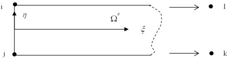
The idea and concept of the elastodynamic infinite ele-ments with united shape functions (for short EIEUSF class infinite elements) are presented in [20,21]. Several EIEUSFformulations are discussed and have been dem-onstrated that the shape functions, related to nodes k and l (the nodes, situated in infinity, Figure 1, are not
neces-sary to be constructed, because corresponding to these shape functions generalized coordinates or weights, see Equation (1), are zeros). The displacements in infinity are vanished, and these shape functions must be omitted. The theory used for the formulation of the EIEUSFclass infinite elements has been published in detail in [6], and hence only summarize of the basic idea is demonstrated here. In [20] is mentioned why the EIEUSFclass infinite elements are more general and powerful than the stan-dard infinite elements.
Figure 1. Local coordinate system of horizontal infinite elements (HIE).
element can be described in the standard form of the shape functions based on wave propagation functions as
1 1
, , , , or
, , , ,
n m
iq iq
i q p
x z N x z
x z N x z
u
u p
p
(1)
where Niq
x z, , are the standard shape displacementfunctions, piq
, ,iq N x z
is the generalized coordinate associ-ated with
, n is the number of nodes for theelement and m is the number of wave functions included
in the formulation of the infinite element. For horizontal wave propagation basic shape functions for the HIE
infi-nite element, the local coordinate system of which is shown in Figure 1, can be expressed as:
, , , , , , ,
, , , ,
iq iq
i q
N x z T x z N
T x z L W
(2)
where Wq
,
are horizontal wave functions and
i
L are Lagrange interpolation polynomial which has unit value at i-th node while zeros at the other nodes. For
HIE infinite element the ranges of the local coordinates are:
1;1
and
0;
. Here T x z
, , ,
as-sures the geometrical transformations of local to global coordinates.
1
, , ,
, , , Re
m
i iq
q
i
N x z N x z
T x z L W
(3)
and
1
, , ,
, , , Re
m
i i iq iq
q
i
N x z N x z
T x z L W
p p
pi
(4)
Then Equation (1) can be expressed as
x z, Np
x z,u p (5)
For horizontal wave propagation the basic shape func-tions for the HIE infinite element can be expressed using
Bessel functions as follows:
, ,
0 qiq i
N L J (6) where J0q
0 0 exp
q q
J J
(7) where J0q
are standard Bessel functions of firstkind. In Equations (6) and (7) and are constants, chosen in such a way that the length of the wave and the attenuation of the wave respectively, are identical with those, if Equation (2) is used. This means that the fol-lowing two relations are valid:
w
w
L
L
or ˆ
(8) where Lw is the wave length if Wq
,
functions are used; π-if Bessel functions of first kind J0
areused (average distance between two zeros) to approxi-mate the displacements in the infinite element domain, and:
1
1
exp exp
(9) because the Bessel functions of first kind attenuate pro-portionally to 1 . The zeros of Bessel functions play a dominant role in applications of these functions [23] and demonstrate their oscillatory. Although the roots of Bessel functions are not generally periodic, except as-ymptotically for large , such functions give acceptable results for simulation of wave propagation. And what is more, using Bessel functions one can approximate change of the wave length in the far field region. If the element has four nodes and eight DOF (the simplest two- dimensional plane element [6]) only four shape functions can be used to approximate the displacements, related to one frequency. These functions can be written as:
1
0
, , , ,
exp or
u
q iq
q i
N N
L J
(10.a)
1q , , iqu , , i 0q
N N L J
(10.b)
2
0
, , , ,
exp or
v
q iq
q i
N N
L J
(11.a)
2q , , iqv , , i 0q
N N L J
(11.b) and
3
0
, , , ,
exp or
u
q jq
q j
N N
L J
(12.a)
3 , , , , 0
u q
q jq j
N N L J
(12.b)
4
0
, , , ,
exp or
v
q jq
q j
N N
L J
(13.a)
are scaling modified Bessel functions of
first kind. These functions can be written as 4
, ,
, ,
0v q
q jq j
where in the general case st 0, 0
0;Lw
.If rotational DOF are used then the element has four nodes and 1o DOF. Two additional shape functions must be used, written as:
5
1 1 0
, , , ,
exp 2
exp
q iq
q q
i q
N N
L J J
J
(14)
and
6
1 1 0
, , , ,
exp 2
exp
q jq
q q
j q
N N
L J J
J
(15)
Here 0
qJ and J1q
are Bessel functions of first kind.The function Li
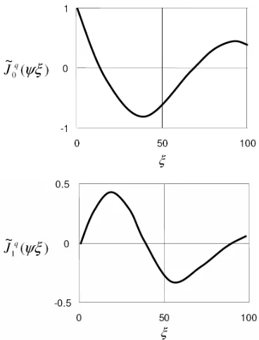
is linear if no mid-nodes. Finally, if mid-node on the side i-j is used, then the Lagrangeinterpolation polynomials must be quadratic. Scaling modified Bessel functions of first kind, in accordance with Equation (6) ( 0
q
J and J1q
), are illus-trated in Figure 2.The continuity along the artificial boundary (the line between finite and infinite elements, see Figure 3 line
b
x
and line xb) is assured in the same way as between
[image:3.595.313.537.85.231.2]two plane finite elements [21]. The application of the proposed infinite elements in the Finite element method is discussed below.
Figure 2. q
J0 and q
J1 scaling modified Bessel functions.
(xb,0) ( ,0)xb
x
c
l
3lc
( )
b
u t
near field far field
infinite elements finite
elements node S
far field
Figure 3. Computational model.
Using the procedure, given in details in [6] and briefly described here, mapped EIEUSFinfinite elements, based on scaling modified Bessel functions, can be formulated, based on Equation (16)
1
1
0 1
, , ,
, , , , ,
, , , m
i iq
q
m
iq q
m
q i q
N x z N x z
T x z N
T x z L J
(16)
where 0
0
exp
q q
J J
.3. Stiffness and Mass Matrices
The matrices ij and ij, related to the near field of
the Soil-Structure System (SSS) can be written as
K M
T d
e
ij i j e
K B DB (17)
and
T d
e
ij i j e
M N N I (18)
and those related to the far field g b
K and Mbg, i.e.
ob-tained for the proposed infinite elements, as
T d
ie
IE IE
g
b i j
ie
K B DB (19)
and
T
d
ie
IE IE g
b i j
M N N ie I (20)
where N, B and D are shape function matrix, strain-dis-
placement matrix and stress-strain matrix, respectively. The matrices Kij and
g b
K are calculated using the
principle of the virtual work.
If Bessel functions are used, the first derivative of
0 q
[image:3.595.80.264.459.701.2]and 1
qJ
the derivative of J0q
) can be ex- pressed) is 0q
q1
1q
2J J
d d
J .The general form of the equations of motion in time domain can be written as
M u t
C u t K f t
u t (21)
[image:4.595.65.290.265.378.2]where M
, C and
K are mass, damping and stiff-ness matrices, respectively, and
f t
[image:4.595.62.285.569.698.2]
s b t t t t a tis nodal force vector.
The equations of motion of the entire SSS, using the
Substructural approach with EIEUSF infinite elements,
based on scaling modified Bessel functions, transformed into time domain by inverse Fourier transformation, are
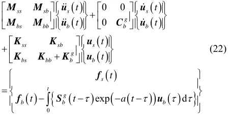
0 0 0 exp d s g b b sb s g b b s gb b b
t t t t t
0 ss sb bs bb ss bs bb t
u u C u K u ff S u
u u
M M M M K KK K (22)
if massless far field is assumed. In Equation (21) u
t and are respectively displacement and force vec-tors, and
t
f ,
g g
b Kb
C and Sbg are matrices of mechanical
characteristics of the far field soil region. Here
0 t
exp d
g g
b t b t
a t
b f
S u (23)can be assumed as a Duhamel integral or more generally as a convolution integral, for t .
Equation (23) is a standard convolution of two func-tions, given in vector forms, namely ub
and fbg
t .Here the vector components of ub
s b t t t t a tcan be taken in case of seismic events from seismograms.
If rotational acceleration of the base is possible, than Equation (22) becomes
0 0 0 exp d s g b b sb s g b b s gb b b
t t t t t t
0 ss sb bs bb ss bs bb t
u u C u K u f ff S u
u u
M M M M K K K K
(24)where f t hm.
The matrix g
t
exp
a t
b
S assures the trans-
formation of the nodal unit displacement impulse vector
ˆb
u , applied at moment , to a nodal force vector
ˆg
b t
f at moment and can be treated as a transfor-
mation matrix, the general form of which can be written as
t
t,T . This matrix in the present case can be
ex-pressed as
exp
g
b t a t
S (25)
where g b
S can be treated as a stiffness matrix, the com-
ponents of which can be calculated from g 2 g b bb
S M .
The vector
g
b t b
f f t denotes the vector of in-teraction forces of the unbounded soil acting at nodes b,
the nodes situated on the artifitual boundary. These forces are acting as a result of the relative motion be-tween the unbounded soil and the total motion of the near field, see Figure 3, expressed in vector forms as
b t
g
b t
u u or
t
t g
t
b
u ub
For discrete time points the vector .
g
b t b t
f f is
calculated, using Equation (26) as
0 exp d g b b t gb b b
t t
t t a t
f f
f S u
(26)
If the force vector, i.e. fbg
t , at moment isknown, i.e.
t
0 exp d t g gb t
b t a t b f S u
t
(27)
at moment t , the force vector can be
obtained using
g b t t
f
0 exp d exp d g b t g b b t t g b b t t tt a t
t t a t t
f S u S u (28) or if t is small time interval using the approximation
0 0 exp d exp d exp g b t g g b b t g b b g b b t tt a t t
t a t
t a t t t
b t
f S u S u S u f (29)If Equation (23) is expressed as
0
sin exp d
t
g g
b t
b t t b f S u
sin t sintcoscostsin
can be used and finally
0
0
cos sin exp d
sin cos exp d
g b
t g
b b
t g
b b
t
t t
t t
f
S u
S u
(31)
Using the proposed infinite elements, the resulting element stiffness matrices related to the far field are in-expensive to calculate and the global stiffness matrix has relatively small bandwidth. It is reasonable to expect similar results in SSI simulations, based on EIEUSF infi-nite elements with modified Bessel shape functions to those when EIEUSFinfinite elements are used.
The nodal displacement vector at moment t can be
calculated using step-by-step method, applied to Equa-tion (23), given in time domain. Such a computaEqua-tional technology is demonstrated in the next Section.
4. Numerical Example
Structure with rigid strip foundation resting on a homo-geneous half-space is modeled as shown in Figure 3,and
the far field is descretized by elastic springs with stiff-ness (model 1), by elastic springs with stiffness
(model 2), by massless EIEUSF infinite elements with
one wave frequency [20] (model 3) and by massless
infi-nite elements with Bessel shape functions [20] (model 4).
1
b
k kb2
Horizontal harmonic displacements with period T and amplitude are applied on the nodes as shown in Figure 3. The geometry of the model
and the material parameters are given in [6].
1 s max 0.25 m
b
u
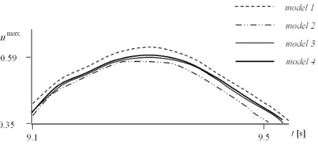
The results for the first 4 natural periods, correspond-ing to the models and max displacement of node S, are given in Table 1. The time history of the displacements
of node S, see Figure 3, between 9.1 s and 9.5 s are
il-lustrated in Figure 4.
The numerical example shows that, if EIEUSF infinite elements or infinite elements with Bessel shape functions are used, the position of xb can be translated starting
from xb 3 Lc (see Lc in Figure 3) to xbLc
with-out significant influence on the results. However, if elas-tic springs are used, the results are significantly affected. Such a reduction of the near field demonstrates the effec-tiveness of the proposed infinite elements.
5. Conclusions
[image:5.595.311.538.83.191.2]In this paper a formulation of elastodynamical infinite element, based on scaled Bessel shape functions, is ap-propriate for Soil-Structure Interaction problem, and the computational concept and the corresponding equations
[image:5.595.309.538.239.329.2]Figure 4. Time history of the displacements of node S.
Table 1. Natural periods, corresponding to the models and max displacements of node S.
Models model 1 model 2 model 3 model 4
1.5628 1.5584 1.5614 1.5615
0.7512 0.7395 0.7455 0.7458
0.5514 0.5377 0.5455 0.5459 natural periods
of vibration
0.2278 0.1985 0.2219 0.2239
max displacement [m] 0.611 0.572 0.585 0.586
of motion of the entire SSI system are presented. This element is a new form of the infinite element, given in [6,21]. The base of the development is new shape func-tions, obtained by modification of the standard Bessel functions of first kind J0
by appropriately chosenscale factor. The stiffness matrices of these infinite ele-ments are calculated by EIEUSF matrix module, and developed by the same author.
The numerical example shows the computational effi-ciency and accuracy of the proposed infinite elements. Such elements can be directly used in the FEM code. The results are in a good agreement with the results, obtained by EIEUSF infinite elements. Moreover, the use of scal-ing modified Bessel functions in the construction of the shape functions leads to computational efficiency in the stage of the calculation of the stiffness and mass infinite element coefficients.
The formulation of 2D horizontal type infinite ele-ments (HIE) is demonstrated, but by similar techniques
2D vertical (VIE) and 2D corner (CIE) infinite elements
can also be formulated. It was demonstrated that the ap-plication of the elastodynamical infinite elements is the easier and appropriate way to achieve an adequate simu-lation (2D elastic media) including basic aspects of Soil- Structure Interaction. Continuity along the artificial boundary (the line between finite and infinite elements) is discussed as well and the application of the proposed elastodynamical infinite elements in the Finite element method is explained in brief.
REFERENCES
Substructure Approach to Soil-Structure Interaction,” Com- putational Mechanics Publications, Vol. 3, Springer Ver-lag, Berlin, 2002.
[2] K. J. Bathe, “Finite Element Procedures in Engineeringa-nalysis,” Prentice-Hill, Upper Saddle River, 1982. [3] U. Basu and A. K. Chopra, “Numerical Evaluation of the
Damping-Solvent Extraction Method in the Frequency Domain,” Earthquake Engineering and Structural Dy-namics, Vol. 31, No. 6, 2002, pp. 1231-1250.
doi:10.1002/eqe.156
[4] P. Bettess, “Infinite Elements,” International Journal for Numerical Methods in Engineering, Vol. 11, No. 1, 1978,
pp. 54-64.
[5] K. Fang and R. Brown, “Numerical Simulation of Wave Propagation in Anisotropic Media,” CREWES Research Report, Vol. 7, 1995.
[6] K. S. Kazakov, “Elastodynamic Infinite Elements with United Shape Function for Soil-Structure Interaction,”
Finite Elements in Analysis and Design, Vol. 46, No. 10,
2010, pp. 936-942. doi:10.1016/j.finel.2010.06.008
[7] J. E. Luco and R. A. Westmann, “Dynamic Response of a Rigid Footing Bonded to an Elastic Half Space,” Journal of Applied Mechanics, Vol. 39, No. 2, 1972, pp. 93-99. doi:10.1115/1.3422711
[8] S. P. G. Madabhushi, “Modeling of Deformations in Dy-namic Soil-Structure Interaction Problems,” VELACS, Tech- nical Report TR277, Cambridge University, Cambridge, 1996.
[9] H. S. Oh and Y. Ch. Jou, “The Weighted Riesz-Galerkin Method for Elliptic Boundary Value Problems on Un-bounded Domain,” NC 28223-0001.
[10] K. S. Kazakov, “Infinite Elements in the Finite Element Method,” 3rd Edition, VSU Publishing House, Sofia, 2010. [11] R. F. Ungless, “Infinite Elements,” M.Sc. Dissertation,
University of British Columbia, Vancouver, 1973. [12] J. P. Wolf and C. Song, “Finite-Element Modeling of
Unbounded Media,” Wiley, London, 1996.
[13] M. C. Genes and S. Kocak, “A Combined Finite Element Based Soil-Structure Interaction Model for Large-Scale
System and Applications on Parallel Platforms,” Engi-neering Structures, Vol. 24, No. 9, 2002, pp. 1119-1131. doi:10.1016/S0141-0296(02)00042-1
[14] K. S. Kazakov, “The Finite Element Method for Struc-tural Modelling,” 2nd Edition, Bulgarian Academy of Sci-ence (BAS) Publishing House, Sofia, 2009.
[15] J. P. Wolf, “Soil-Structure Interaction Analysis in a Time Domain,” Prentice-Hill, Englewood Cliffs, 1988. [16] Ch. B. Yan, D. K. Kim and J. N. Kim, “Analytical
Fre-quency-Dependent Infinite Elements for Soil-Structure Interaction Analysis in a Two-Dimensional Medium,”
Engineering Structures, Vol. 22, No. 3, 2000, pp. 258-
271. doi:10.1016/S0141-0296(98)00070-4
[17] Ch. Zhao and S. Valliappan, “A Dynamic Infinite Ele-ment for Three-Dimensional Infinite Domain Wave Prob-lems,” International Journal for Numerical Methods in Engineering, Vol. 36, No. 15, 1993, pp. 2567-2580. doi:10.1002/nme.1620361505
[18] K. S. Kazakov, “Formulation of Elastodynamic Infinite Elements for Dynamic Soil-Structure Interaction,” WSEAS Transactions on Applied and Theoretical Mechanics, Vol.
6, No. 1, 2011, pp. 91-96.
[19] K. S. Kazakov, “Mapping Functions for 2D Elastody-namic Infinite Element with United Shape Function,” Slo-vak Journal of Civil Engineering, Vol. 16, 2008, pp. 17-
25.
[20] K. S. Kazakov, “On an Elastodynamic Infinite Element, Appropriate for an Soil-Structure Interaction Models,”
Proceedings of 10th Jubilee National Congress on Theo-retical and Applied Mechanics, Varna, Vol. 1, 2005, pp.
230-236.
[21] K. S. Kazakov, “Stiffness and Mass Matrices of FEM- Applicable Dynamic Infinite Element with Unified Shape Basis,” AIP Conference Proceedings, Vol. 1138, No. 1, 2009, p. 95. doi:10.1063/1.3155133
[22] P. K. Pradhan, D. K. Baidya and D. P. Ghosh, “Imped-ance Functions of Circular Foundation Resting on Soil Using Cone Model,” ASMEReport 12, 2003.