Exploring Deep Reinforcement Learning with Multi Q Learning

ISSN Online: 2153-0661 ISSN Print: 2153-0653

Exploring Deep Reinforcement Learning with

Multi Q-Learning

Ethan Duryea, Michael Ganger, Wei Hu

Department of Computer Science, Houghton College, Houghton, USA

Abstract

Q-learning is a popular temporal-difference reinforcement learning algorithm which often explicitly stores state values using lookup tables. This implementation has been proven to converge to the optimal solution, but it is often beneficial to use a func-tion-approximation system, such as deep neural networks, to estimate state values. It has been previously observed that Q-learning can be unstable when using value func-tion approximafunc-tion or when operating in a stochastic environment. This instability can adversely affect the algorithm’s ability to maximize its returns. In this paper, we present a new algorithm called Multi Q-learning to attempt to overcome the instabil-ity seen in Q-learning. We test our algorithm on a 4 × 4 grid-world with different stochastic reward functions using various deep neural networks and convolutional networks. Our results show that in most cases, Multi Q-learning outperforms Q- learning, achieving average returns up to 2.5 times higher than Q-learning and hav-ing a standard deviation of state values as low as 0.58.

Keywords

Reinforcement Learning, Deep Learning, Multi Q-Learning

1. Introduction

Reinforcement learning is a form of machine learning in which an agent attempts to learn a policy that maximizes a numeric reward signal [1]. In reinforcement learning, an agent learns by trial and error and discovers optimal actions through its own expe-riences. Unlike supervised learning, the agent does not learn by comparing its own ac-tions to those of an expert; everything it learns is from its own interacac-tions with the en-vironment. Reinforcement learning attempts to solve optimization problems that are defined by a Markov Decision Process (MDP) [1]. A Markov Decision Process defines the behavior of the environment by mathematically defining the environment’s one- How to cite this paper: Duryea, E., Ganger,

M. and Hu, W. (2016) Exploring Deep Rein-forcement Learning with Multi Q-Learning. Intelligent Control and Automation, 7, 129- 144.

http://dx.doi.org/10.4236/ica.2016.74012

Received: August 9, 2016 Accepted: November 12, 2016 Published: November 15, 2016

Copyright © 2016 by authors and Scientific Research Publishing Inc. This work is licensed under the Creative Commons Attribution International License (CC BY 4.0).

http://creativecommons.org/licenses/by/4.0/

step dynamics. There are three main categories of reinforcement learning algorithms: dynamic programming, Monte Carlo, and temporal-difference (TD) [1]. Temporal- difference learning algorithms are central to the domain of reinforcement learning and will be the focus of this paper.

Q-learning is one of the most popular TD algorithms [1]. Like many other rein-forcement learning algorithms, Q-learning is model-free, which means it learns a con-troller without learning a model. To learn this concon-troller, Q-learning trains an ac-tion-value function that returns the expected value for taking action a in state s. The agent will use this function to form a policy which will maximize returns. The Q-value for a state-action pair is given by the Bellman equation

( )

(

)

, max ,

a

Q s a E r γ Q s a ′

 _{′ ′} 

= _ + _ (1)

where r is the observed reward after performing a in s, γ _{is a constant discount factor}

0≤ ≤γ 1, and s′ is the transition state after performing a in s. Q-learning updates its

Q-values by comparing its new estimates to its existing estimates; the new estimate (target) for Q-learning is

(

)

1 max 1,

t t

a

r₊ +γ Q s₊ a (2)

where t is the current time-step during training. Thus, the update for the Q-value of the state-action pair

(

)

(

)

(

)

(

)

(

)

Q s a ←Q s a +α_r+ +γ Q s+ a −Q s a _ (3)

where α is the learning rate.

Q-learning is a critical algorithm in reinforcement learning and has been successfully applied to a large number of tasks, but it has also been observed that the algorithm will sometimes overestimate the optimal Q-values. This overestimation occurs when the reward function of the MDP is stochastic. Double Q-learning is a variation to Q- learning that addresses this problem [2]. The overestimation is due to Q-learning’s use of the max operator to select and evaluate the actions of the next state. Double Q-learning attempts to fix this issue by using two Q functions, A

Q and B

Q to

de-couple the selection and evaluation of the action in the next state. To accomplish this, Double Q-learning uses the value of B

Q to update A

Q , so the update for A Q

be-comes

( )

( )

(

)

( )

A A B A A

a

Q s a ←Q s a +α_r+γQ _s′ Q s a′ _−Q s a _

 

  (4)

The roles of A

Q and QB are switched when updating QB. Double Q-learning

of-ten develops better value estimates and achieves greater performance compared to Q-learning on certain stochastic tasks [2].

ac-tions. In the case of a high-dimensional MDP, function approximation is generally used. Q-learning, as well as other off-policy TD algorithms, can be unstable with linear/ non-linear function approximation [4] [5] [6] [7].

Artificial neural networks are one effective method of function approximation. These neural networks are mathematical models made up of parameters that are tuned using back-propagation. Deep learning is a variety of artificial neural networks and has seen great success in learning from high-dimensional data, specifically image recognition [8], Natural Language Processing [9], and facial recognition [10]. The artificial neural net-works used in deep learning have many layers of parameters which can be either fully connected, convolutional, or recurrent layers [11]. Coupling deep learning with rein-forcement learning allows agents to find optimal policies for complex, high-dimen- sional tasks. This has enabled agents to learn using raw pixels as input, which allows for the agents to learn a variety of tasks without needing to tune parameters or adjust the state representation for each individual task. Deep neural networks have brought us closer to the goal of creating a general purpose artificial intelligence.

AlphaGo is a computer program developed by Deep Mind that utilized deep learning along with a Monte Carlo search tree to play Go [12]. Go is an ancient Chinese game where the number of possible board configurations is 2.08168199382 × 10170. Without the use of deep learning AlphaGo would never have been so successful at playing such a complex game. Apart from AlphaGo, two of most widely-known successes of rein-forcement learning are TD-gammon; a program that learned how to play backgammon at a super-human level [13], and DQN; a Q-learning algorithm that used a deep neural network to achieve a super-human level of play at several Atari 2600 games [14]. Both of these algorithms demonstrated the benefits of using artificial neural networks as val-ue functions.

Deep reinforcement learning has also been successfully applied to continuous control problems. By combining deep neural networks with the actor-critic algorithm [1], the Deep DPG algorithm was able to learn competitive policies for a variety of physics tasks including cart-pole swing-up, car driving, legged locomotion, and others [15]. The ad-vantages of using deep learning with reinforcement learning are great, which is why it is important to have an algorithm that is capable of remaining stable when using deep neural networks as value functions.

As mention earlier, the instability of value estimates is one of the biggest challenges to overcome when using linear/nonlinear value function approximation. To combat this instability issue, algorithms that use neural networks as their Q functions often train using

(

)

Instead of using any of the previously mentioned techniques, we attempt to achieve robust value estimates by introducing a new TD algorithm called Multi Q-learning. Our algorithm outperforms Q-learning and Double Q-learning in our tests and provides more stable Q-values throughout the training process. Multi Q-learning also works well with a diverse range of neural network implementation, making the algorithms benefi-cial when the ideal network structure is unknown. We find the Multi Q-learning algo-rithm to be an effective alternative to Q-learning due to its robustness and stability.

2. Methods

In this paper we discuss a new TD algorithm that extends upon Q-learning and Double Q-learning called Multi Q-learning. The main idea behind this new algorithm comes from Double Q-learning’s use of two estimators to find the maximum expected value for each action. Instead of simply using two Q functions: QA _{and Q}B_{, Multi Q-learning}

uses an arbitrary number of Q functions to estimate the action values. The algorithm updates one Q function at each time-step using the average value of all the other Q functions. So when Multi Q-learning contains a list of n Q-functions, and A∈

{

}

then the update for QA _becomes

( )

(

)

( )

1

1,

1

, , arg max , ,

1 n

A A b A A

t t t t t

a b b A

Q Q s a r Q s Q s a Q s a

n α γ + = ≠  _{ ′ ′ }  = + _ + _{ }− _ −  



∑

The purpose of using multiple Q functions is to better stabilize the target value. Double Q-learning uncouples the selection and evaluation of an action, creating an un-biased estimate for the value of that action. But any drastic change in one Q function will greatly affect the other. Multi Q-learning addresses this problem by using the aver-age action-value of many Q functions to update a specific Q function. If there is a dras-tic change in an action-value of one Q function, its effect on the other Q functions will be minimal. This helps when a substantial amount of noise exists in the environment, specifically in the environment’s reward function. Our Multi Q-learning algorithm is presented in Algorithm 1 below.

Algorithm 1. Multi Q-learning. 1: Initialize 1 2

,

, , n

Q Q Q arbitrarily 2: for episode = 1, M do

3: Initialize s

4: Repeat

5: Choose _QA where _A∈{_{1, 2,}_,n} using probability 1

n 6: Choose a from s using policy derived from _QA (e.g., ε-greedy)

7: Take action a, observe r s, ′

8: * ( )

arg max A , a

a = Q s a′

9: ( )

(

)

1,

1

, , ,

1

n

A A b A

b b A

Q Q s a r Q s a Q s a

n α γ = ≠  _′  ← + _ + − _ − 

∑

10: s←s′

11: until𝑠𝑠 is terminal

The algorithm for Multi Q-learning is quite similar to Double Q-learning. The key difference is the use of n Q functions opposed to only two. At each step in a training episode, we choose a single Q function to update based on the probability 1

n so that each Q function is chosen to be updated with an equal probability. After the training is finished, the Q-value for each state-action pair becomes the average Q-value of all the Q functions.

Similarly to Q-learning and Double Q-learning’s extension to DQN and Double DQN [17], Multi Q-learning can naturally be extended to utilize deep neural networks. The benefits of deep reinforcement learning have been realized by many studies [11]. Pairing deep neural networks with Multi Q-learning allows for stability while learning complex relationships between the features of a state.

In the original Double DQN algorithm, the weights of a target network θt − _were

used to estimate the value of the greedy-policy and update the weights of the online network θt. The target network weights were simply copied from the online network every τ steps. The target used by Double DQN is

(

)

Double DQN

1 1, arg max 1, ; ,

t t t t t t

a

Y ≡r₊ +γQ s_{ +} Q s₊ aθ θ−_

  (6)

For the Deep Multi Q-learning algorithm, we created an independent neural network for each Q. This fully decouples the selection and evaluation of an action, unlike Double DQN which only was partially decoupled. The target used by the Deep Multi Q-learning algorithm for a network characterized by weights θA _where

{

}

1, 2, ,

A∈  n is

(

)

1 1 1

1, 1

, argmax , ; ; 1

n

A b

t t t t t t

a b i A

Y r Q s Q s a

n

γ θ θ

+ + +

= ≠

≡ _ _

 +

−

∑

For our Deep Multi Q-learning algorithm, show in Algorithm 2 below:

Algorithm 2. Deep Multi Q-learning. 1: Initialize θ1_{, ,}θn−1_,θn

 arbitrarily

2: for episode = 1, M do 3: Initialize s

4: Repeat

5: Choose θA where _A∈{_{1, 2,}_,n} using probability 1

n

6: Choose a from s using policy derived from

(

)

Q s aθ (e.g., ε-greedy)

7: Take action a, observe r s, ′

8: *

(

)

arg max , ; A a

a = Q s a′ θ

9:

(

)

1, 1 , ; 1 n A b

b b A

y r Q s a

n γ θ = ≠ ′ = + −

∑

10 Train network using _yA,θA,_s

11: s←s′

12: until𝑠𝑠 is terminal

3. Results

In this section, we analyze the performance of Q-learning, Double Q-learning, and Multi Q-learning. The metrics we focus on are the value estimates, the average returns, and the success rates. Our results show the robustness of Multi Q-learning when faced with stochastic rewards and that this robustness increases the performance of the algo-rithm. We also show the instability of Q-learning and Double Q-learning and how that instability can negatively affect the overall performance of the algorithm.

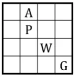
A 4 × 4 grid world (Figure 1) was used to evaluate the algorithms. Each state has 4 actions, corresponding to the directions the agent can move. The world has 2 terminal states, a pit and a goal, which return rewards of −10 and 10 respectively. A wall was added to the grid which blocks the movement of the agent into that location. If the agent took an invalid action, such as moving into the boundary or wall, the agent did not move and simply remained in the same position. The objective of the agent was to navigate from its starting position to the goal in the shortest amount of moves without falling into the pit. Every non-terminal state returned an average reward µ with standard deviation σ. To compare, we show the difference between algorithms for rewards with deterministic distribution p

(

)

values p

(

)

(

)

{

}

the algorithms using two different behavior policies. One policy was strictly exploratory while the other was ε-greedy. For the ε-greedy policy, ε was initialized to 1 and reduce by 1/100,000 at the end of each episode until ε = 0.1.

The grid world was initialized to the same state at the start of every game. A training episode ends when the agent reaches a terminal state, whether it is the goal or the pit. The algorithms trained for 100,000 episodes and at the end of each episode, we ran the learned policy on the task and recorded the total return and the number of steps taken. If the agent fell into the pit, or took more than 10 steps, a 0 was record for the number of steps taken. The results were averaged over every 100 episodes in order to smooth the graphs.

3.1. Neural Network Results

In the following section, we evaluate our algorithm using a neural network with two hidden layers for the value function. One-hot encoding was used to represent the state as a 64 vector where the position of each object corresponded to a 16 element slice of

that vector. The vector representation of the state was used as the input to our neural network. Both hidden layers were fully connected and consisted of 150 rectifier units. The output layer was a fully connected linear layer with an output for each move. We used the RMSProp gradient descent algorithm [18] to optimize the network and trained after each time-step.

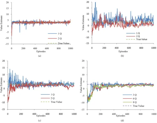
Figure 2(a) and Figure 2(b) show the value estimates of both Double Q-learning and Q-learning. These values estimates are for the initial state of the grid world and were averaged out over every 100 episodes in order to smooth the graph. Both Double Q- learning and Q-learning converged toward the true value of 3.1 quickly when the re-ward function was deterministic (Figure 2(a)). But when faced with a stochastic reward (σ =7), the value estimates contain a substantial amount of oscillation (Figure 2(b)). When using the ε-greedy behavior policy, the oscillation of the value estimates was re-

(a) (b)

(c) (d)

Figure 2. Value estimate for Q-learning, Double Q-learning, and Multi Q-learning. (a) The value estimate of the initial state where 1

duced as the training progressed (Figure 2(c)) due to the decreased amount of explo-ratory moves taken. Figure 2(d) shows the value estimates of three Multi Q-learning algorithms using the same environment parameters as Figure 2(c). It is easy to see the stability in the value estimates of the Multi Q-learning algorithm; the value estimates quickly converge to the true value of the state, 3.1, and have small amount of oscillation. In the early stages of learning, Figure 2(c) shows the significant amount of oscillation in Q-learning’s value estimates. This oscillation is due to the stochastic reward function. Like Multi Q-learning, Double Q-learning’s value estimate converges quickly to the true value and remains relatively stable throughout the training process. Unlike Multi Q-learning, Double Q-learning’s value estimate starts to decline at around 900 episodes. While this is just a slight oscillation and the value estimate eventually rises back to the true value, it does show that Multi Q-learning has an advantage over Double Q-learn- ing in stability.

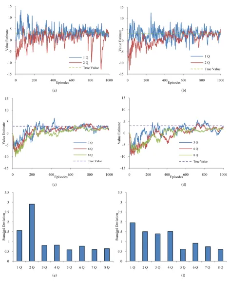
When the standard deviation of the reward function was increased, the deviation in the value estimate increased for each algorithm. When using an𝜀𝜀-greedy behavior pol-icy, Q-learning and Double Q-learning eventually converged to the true value, but with more oscillation compared to Multi Q, especially within the early stages of learning. When actions were completely exploratory, the variance in the value estimates of Q- learning and Double Q-learning greatly increased which caused both algorithms to struggle in approximating the true value. Multi Q-learning’s estimates steadily con-verged toward the true value and eventually stabilized even when faced with a greater range of rewards (Figure 3(c) and Figure 3(d)). This stability increase can clearly be seen in the decrease of standard deviation in the value estimates after 50,000 episodes (Figure 3(e) and Figure 3(f)). The increase of estimators slowed the convergence rate; this is due to only one network being trained at a time, so with the addition of more es-timators the less frequent their respective network gets updated.

(a) (b)

(c) (d)

(e) (f)

Figure 3. Value estimates and their respective standard deviation of Single Q-learning, Double Q-learning, and Multi Q-learning. (a) (b) Value estimates of Q-learning and Double Q-learning of the initial state where the behavior policy is ε-greedy, µ= −1 and σ=13,15 for the respective figures. (c) (d) Value estimates of 3 Multi Q-learning algorithms of the initial state where the behavior policy is ε-greedy,

1

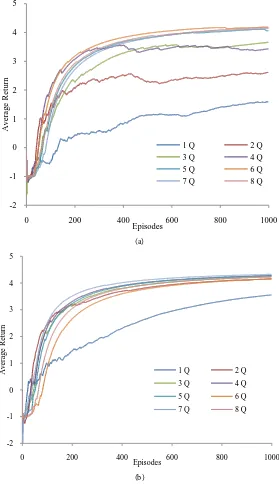
The oscillation in the value estimates had quite an effect on Q-learning and Double Q-learning’s performance. Figure 4 shows the average return curve of all three algo-rithms. When the standard deviation of the reward function was 7 and the policy was exclusively exploratory, Q-learning and Double Q-learning both performed poorly.

Figure 4(b) shows the return curves of each algorithm when using the ε-greedy policy.

(a)

(b)

Figure 4. Average return curves for Q-learning, Double Q-learning, and Multi Q-learning. (a) The average return curve for each algorithm where the behavior policy was random, µ= −1 and σ =7; (b) The average return curve for each algorithm where the behavior policy was

ε-greedy, µ= −1 and σ =7. -2

-1 0 1 2 3 4 5

0 200 400 600 800 1000

A

v

er

ag

e R

et

u

rn

Episodes

1 Q 2 Q

3 Q 4 Q

5 Q 6 Q

7 Q 8 Q

-2 -1 0 1 2 3 4 5

0 200 400 600 800 1000

A

v

er

ag

e R

et

u

rn

Episodes

1 Q 2 Q

3 Q 4 Q

5 Q 6 Q

There was no noticeable difference between Double Q and Multi Q while Q-learning clearly performed the worst. Multi Q-learning performed noticeably better when a random action was always taken. Q-learning had an average return of 1.1, Double Q’s average return was 2.4, and all the Multi Q algorithms had average returns above 3.5 when the behavior policy always choose a random action. This demonstrates Multi Q’s stability regardless its behavior policy.

The high returns are due to Multi Q’s ability to consistently reach the goal through-out its training. The success rates shown in Table 1 indicate Multi Q-learning per-formed better than Q-learning and Double Q-learning. For a reward function with

7

σ = _{and a strictly exploratory behavior policy, Q-learning failed to reach the goal} over 50% of the time. Double Q-learning did not fare much better and only succeeded 65.5% of the time, while 8 Q performed very well with a success rate of 94.2%. As stated before, when using an ε-greedy policy, there was no noticeable difference between Double Q-learning and Multi Q-learning. But when σ was increased, the success rates of Q-learning, Double Q-learning, and Multi Q-learning became clearly different. At the highest reward function deviation we trained on, σ =19, Q-learning’s success rate was 60.8%, Double Q-learning’s was 75.8%, and 3 Q-learning’s was 88.1%. We also see that as σ increased, Multi Q-learning’s success rate decreased at a lower rate than both Q-learning and Double Q-learning. This shows that Multi Q’s stable value esti-mates result in more successful agents.

It is also interesting to note the smoothness of the return curve as the number of es-timators increase. Using 4 or more eses-timators creates a much smoother curve than us-ing 1, 2, or even 3. This smoothness can again be attributed to the stability of Multi Q’s value function approximation. The algorithm steadily converges to the optimal value estimate and has very little fluctuation.

In addition to the neural networks used above, we used three other network archi-tectures to approximate each algorithm’s value function. We demonstrate the benefit of adding convolutional layers to improve value approximation. The first architecture we used had two fully connected hidden layers, both of size ten. The next network replaced the first hidden layer with a convolutional layer. This convolutional layer had ten filters

Table 1. Success rates for each algorithm with different reward function standard deviations.

𝜎𝜎 Algorithm

1 Q 2 Q 3 Q 4 Q 5 Q 6 Q 7 Q 8 Q

7 82.4% 93.3% 94.6% 95.4% 95.3% 93.2% 96.3% 94.6%

9 75.2% 88.3% 94.9% 94.8% 92.7% 93.2% 92.7% 92.6%

11 70.7% 85.9% 92.3% 90.1% 89.1% 92.5% 90.0% 91.4%

13 68.4% 81.3% 87.6% 93.4% 92.6% 93.1% 89.8% 91.0%

15 57.9% 81.7% 85.6% 87.3% 87.3% 90.9% 87.5% 84.7%

17 65.8% 77.9% 87.0% 83.7% 85.6% 87.5% 85.8% 81.2%

all with a length of five. The addition of a convolutional layer slightly improved upon the network’s value estimates, leading to higher average returns. The final neural net-work had three hidden layers. These hidden layers were all fully connected and had a size of ten. Having three hidden layers did not improve upon any of the algorithms’ av-erage returns. In fact, the addition of another layer actually performed worse than hav-ing only two hidden layers. Figure 5 shows the comparison of the different network architectures’ average returns.

The average returns of the algorithms demonstrate an important advantage Multi Q-learning has over both Double Q-learning and Q-learning. The average returns of both Double Q-learning and Q-learning decreased steadily with the different neural network structures used. In our grid world environment, these two algorithms per-formed the best with two fully connected layers. Using this structure, Q-learning had an average return of 0.59 and Double Q-learning had an average return of 3.19. The algo-rithms’ performances dropped when a network structure of one convolutional layer and one fully connected layer was used. In this case, Q-learning had an average return of 0.52 and Double Q-learning had an average return of 2.79. The algorithms perform the worst when the network structure was made up of three fully connected layers. With this structure, Q-learning’s average return was 0.02 and Double Q-learning’s av-erage return was 1.86. The decrease in avav-erage returns of Q-learning and Double Q-learning is in contrast Multi Q-learning. The Multi Q-learning algorithms did not see any major decrease in average returns when faced with different neural networks. This is a clear advantage of Multi Q-learning compared to Double Q-learning and Q- learning. The Multi Q algorithm is not as easily effected by the type of network struc-ture or function approximator used to estimate the value function.

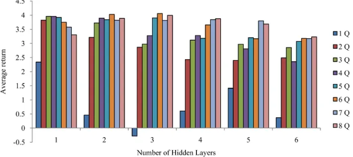
To further demonstrate the robustness of the Multi Q-learning algorithm, we show the average return of the algorithms with neural networks of increasing depth. Figure 6

Figure 6. The average return of each algorithm using a neural network to approximate the value function. Each layer of the neural network contains 85 rectified linear units and increases in depth. This graph shows the stability of the Multi Q-learning algorithm regardless of the depth of the network.

shows the average returns of each algorithm as the number of hidden layers in the net-work increased. The behavior policy during these tests was exclusively random, so the agent always took a random action throughout training. The performance of both Q-learning and Double Q-learning declined as the number of layers in the network in-creased. Contrarily, the performance of 6 Q, 7 Q and 8 Q remained relatively stable re-gardless of the number of layers. The returns for 6 Q, 7 Q, and 8 Q began to decrease once the network reached a depth of 5 hidden layers. This poor performance can likely be attributed to the vanishing gradient problem with neural networks. This again shows the stability and robustness of the Multi Q-learning algorithm; despite the depth of the network, Multi Q-learning is still able to solve the problem and achieve high returns.

3.2. Tabular Results

We also ran the Multi Q-learning algorithm using Q-tables in addition to neural net-works. The results of using Q-tables were less drastic then those found with the neural networks, but we did find a slight advantage of Multi Q-learning. In the early stages of training, Multi Q-learning appeared to have developed better policies than Q-learning and Double Q-learning. Figure 7(a) shows the average return of each algorithm after 2000 episodes. At 2000 episodes, Q-learning had an average return of −1, meaning that it has failed to reach the goal even once up to this point. Double Q-learning did much better with an average return of 2.2. The performance of 5 Q was the best, having an average return of 3.6 at 2000 episodes.

4. Conclusion

(a)

(b)

Figure 7. The average return of Q-learning, Double Q-learning, and Multi Q-learning when us-ing Q-tables. (a) Average return after 2000 episodes of each algorithm usus-ing Q-tables. In this ex-periment µ= −1,σ=11 and the behavior policy was random; (b) Average return curves of each algorithm from the same experiment as (a).

Q-learning. In our tests, Multi Q-learning achieved better average returns compared to Q-learning, reaching returns up to 2.6 times higher than Q-learning. We also ran Multi Q-learning on various neural network structures, including deep, shallow, and convo-lutional networks, demonstrating the algorithms ability to remain effective despite its implementation. While Double Q-learning and Q-learning performance decreased with ineffective implementation, Multi Q-learning was still able to retain good returns. We see Multi Q-learning being most useful when the dynamics of a reinforcement learning task are not well known. Multi Q-learning’s improved stability over Q-learning makes

-1 0 1 2 3 4

1 Q 2 Q 3 Q 4 Q 5 Q 6 Q 7 Q 8 Q

A

v

er

ag

e R

et

u

rn

-2 -1 0 1 2 3 4 5

0 10 20 30 40 50

A

v

er

ag

e R

et

ru

n

Episodes x100

1 Q 2 Q 3 Q

4 Q 5 Q 6 Q

it a more generalize algorithm, being able to solve a variety of tasks without the need to tune its parameters.

Acknowledgements

We would like to thank the Summer Research Institute at Houghton College for pro-viding financial support for this study.

References

[1] Sutton, R.S. and Barto, A.G. (1998) Reinforcement Learning: An Introduction, Vol. 1. MIT Press, Cambridge.

[2] Hasselt, H.V. (2010) Double Q-Learning. Advances in Neural Information Processing Sys-tems, 2613-2621. http://papers.nips.cc/paper/3964-double-q-learning

[3] Watkins, C.J.C.H. and Dayan, P. (1992) Q-Learning. Machine Learning, 8, 279-292. http://dx.doi.org/10.1007/BF00992698

[4] Baird, L. (1995) Residual Algorithms: Reinforcement Learning with Function Approxima-tion. Proceedings of the Twelfth International Conference on Machine Learning, Tahoe City, California, 9-12 July 1995, 30-37.

[5] Tsitsiklis, J.N. and Van Roy, B. (1997) An Analysis of Temporal-Difference Learning with Function Approximation. IEEE Transactions on Automatic Control, 42, 674-690.

http://dx.doi.org/10.1109/9.580874

[6] Maei, H.R., et al. (2011) Gradient Temporal-Difference Learning Algorithms.

http://incompleteideas.net/rlai609/slides/gradient%20TD%20slides.pdf

[7] Sutton, R.S., Mahmood, A.R. and White, M. (2015) An Emphatic Approach to the Problem of Off-Policy Temporal-Difference Learning. The Journal of Machine Learning Research, 17, 1-29.

[8] Simonyan, K. and Zisserman, A. (2014) Very Deep Convolutional Networks for Large-Scale Image Recognition. arXiv preprint arXiv:1409.1556

[9] Collobert, R. and Weston, J. (2008) A Unified Architecture for Natural Language Processing: Deep Neural Networks with Multitask Learning. Proceedings of the 25th

Inter-national Conference on Machine Learning, Helsinki, 5-9 July 2008, 160-167.

[10] Sun, Y., Wang, X. and Tang, X. (2014) Deep Learning Face Representation from Predicting 10,000 Classes. Proceedings of the IEEE Conference on Computer Vision and Pattern

Rec-ognition, Columbus, 23-28 June 2014, 1891-1898. http://dx.doi.org/10.1109/9.580874

[11] LeCun, Y., Bengio, Y. and Hinton, G. (2015) Deep Learning. Nature, 521, 436-444. http://dx.doi.org/10.1038/nature14539

[12] Silver, D., Huang, A., Maddison, C.J., Guez, A., Sifre, L., Van Den Driessche, G., Schritt-wieser, J., Antonoglou, I., Panneershelvam, V., Lanctot, M., et al. (2016) Mastering the Game of Go with Deep Neural Networks and Tree Search. Nature, 529, 484-489.

http://dx.doi.org/10.1038/nature16961

[13] Tesauro, G. (1995) Temporal Difference Learning and TD-Gammon. Communications of

the ACM, 38, 58-68. http://dx.doi.org/10.1145/203330.203343

[14] Mnih, V., Kavukcuoglu, K., Silver, D., Rusu, A.A., Veness, J., Bellemare, M.G., Graves, A., Riedmiller, M., Fidjeland, A.K., Ostrovski, G., et al. (2015) Human-Level Control through Deep Reinforcement Learning. Nature, 518, 529-533.

[15] Lillicrap, T.P., Hunt, J.J., Pritzel, A., Heess, N., Erez, T., Tassa, Y., Silver, D. and Wierstra, D. (2015) Continuous Control with Deep Reinforcement Learning.

arXiv preprint arXiv:1509.02971

[16] Mnih, V., Kavukcuoglu, K., Silver, D., Graves, A., Antonoglou, I., Wierstra, D. and Ried-miller, M. (2013) Playing Atari with Deep Reinforcement Learning.

arXiv preprint arXiv:1312.5602

[17] Van Hasselt, H., Guez, A. and Silver, D. (2015) Deep Reinforcement Learning with Double Q-Learning. arXiv:1509.06461 [cs.LG]

[18] Tieleman, T. and Hinton, G. (2012) Lecture 6.5-rmsprop: Divide the Gradient by a Running Average of Its Recent Magnitude. COURSERA: Neural Networks for Machine Learning, 4, 26-31.

Submit or recommend next manuscript to SCIRP and we will provide best service for you:

Accepting pre-submission inquiries through Email, Facebook, LinkedIn, Twitter, etc. A wide selection of journals (inclusive of 9 subjects, more than 200 journals)

Providing 24-hour high-quality service User-friendly online submission system Fair and swift peer-review system

Efficient typesetting and proofreading procedure

Display of the result of downloads and visits, as well as the number of cited articles Maximum dissemination of your research work

Submit your manuscript at: http://papersubmission.scirp.org/