A Comparative Study of Amplitude and Timing
Estimation in Experimental Particle Physics using
Monte Carlo Simulation
Hongda Xu1, Datao Gong2, Yun Chiu1
1Departmentof Electrical Engineering, University of Texas at Dallas, Richardson, TX, USA 2Departmentof Physics, Southern Methodist University, Dallas, TX, USA
Email: [email protected]
Received 2013
ABSTRACT
Optimal detection of liquid ionization calorimeter signal in experimental particle physics is considered. A few linear and nonlinear approaches for amplitude and arrival time estimation based on the χ2 function are compared in simulation considering the noise sample correlation introduced by the analog pulse shaper. The estimation bias of the first-order approximation, a.k.a linear optimal filtering, is studied and contrasted to those of the second-order as well as the ex-haustive search. A gradient-descent technique is presented as an alternative to the exex-haustive search with significantly reduced search time and computation complexity. Results from various pulse shapers including the CR-RC2, CR-RC3, and CR2-RC2 are also compared.
Keywords: Liquid Ionization Calorimeter; Detection; Optimal Filtering; Amplitude and Timing Estimation; χ2 Function; CRm-RCn pulse Shaper; Linear Optimal Filtering; Exhaustive Search; Gradient Descent; Monte Carlo
1. Introduction
In particle physics experiment, it is common to measure the small charge signal collected by the detector in pres-ence of electronic noise. A collection of data acquisition and signal processing techniques are well developed to optimize the singal-to-noise ratio (SNR) in such systems [1]. Due to the recent development of optical transmis-sion techniques, a trend in detector readout system design is to continuously digitize the detector signal and con-tinuously transmit the data out of the front-end to the control room, in which complex signal processing can be imposed to improve the overall detector system per-formance [2]. This paper reviews several of such signal processing techniques for liquid ionization calorimeters and compares their performance in simulation. A novel accurate, fast, and low-cost gradient-descent technique is also introduced in the paper.
2. Liquid Ionization Calorimeter
Liquid ionization calorimeter is an energy-measurement detector widely deployed in many particle physics ex- periments [3-6]. Since the liquid gap between the elec-trode plates is narrow, e.g., about 2 mm in ATLAS liquid argon calorimeter, the ionization triggered by the
electromagnetic shower is instantaneous and the process is followed by a drift of the electrons towards the anode plate. Thus, the detector output signal is modeled as a tri-angular current pulse. Liquid ionization calorimeter usu-ally exhibit so long drift time, dependent on the drift ve-locity and the gap size [7]. For example, the drift time in AT- LAS liquid argon calorimeter is about 450 ns, much longer than the bunch crossing time which is 25 ns. To avoid long dead time and to reduce noise in the meas- urement, a CRm-RCn pulse shaper – a chain of integrator (RC) and differentiator (CR) circuits – is always employed in the analog front-end before digitalization [8]. The gen-eral transfer function of a CRm-RCn shaper is given as follows.
1
m s
m n s
s H s
s
(1)
where τs is the time constant of the shaper. An intuitive
output waveform with minimal pedestal recovering time, which can largely relax the ADC sample rate while re-taining sufficient samples for post-processing.
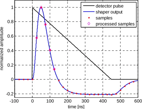
Figure 1 sketches the shaped waveform as well as the triangular current pulse from the detector. The parame-ters used for modeling waveforms in Figure 1 are ex-tracted from [9] for ATLAS liquid argon calorimeter, e.g., a CR-RC2 shaper with τ
s set to 13 ns, and the output
peaking time is approximately 50 ns.
3. Detection and Signal Processing
While detection is a general signal-processing topic that has been well studied, what we are most interested in par-ticle physics experiments is how to precisely measure the
amplitude and timing information of the sampled wave- form of the detector output – the amplitude A represents the energy of the incident particle shower and the timing signifies the arrival time τ of the particle thus our ability to correlate signals and events in time.
The general approach of determining amplitude and timing information from limited number of samples can be derived from the theory of optimal filtering [1,10]. The technique in the core constitutes a search algorithm to project the samples to the known signal space of the detector front-end including the preamplifier, the shaper, and the analog-to-digital converter to maximize the SNR of the detected signal. Two leading noises are typically considered in the optimization process, the electronic noise and the pileup noise. At their origin, the dominant electronic noises, e.g., thermal noise and shot noise, are white. Temporal correlation however is introduced by the detector front-end processing, particularly the pulse shaper, and needs to be considered in the optimization procedure. Unlike the stochastic deteriorating effect of
-100 0 100 200 300 400 500 600
-0.2 0 0.2 0.4 0.6 0.8 1
time [ns]
nor
m
al
iz
ed am
pl
it
ude
detector pulse shaper output samples
processed samples
Figure 1. The triangular current pulse produced by a liquid ionization calorimeter and the output waveform of the analog pulse shaper. The five samples (at the sample rate of 40 MS/s) for post-processing are highlighted.
the electronic noise, the signal pileup by nature is deter- ministic and should be treated as inter-event interference
(IEI). In particle detectors operating at high luminosity levels, many events are produced at each bunch crossing. The densely packed calorimeter cells and the long tail of the detector current pulse tend to aggravate the IEI prob-lem, leading to an equivalent model termed pileup noise to highlight the statistical property of the effect rather than its deterministic physical origin.
Many works have been reported for detetctor signal processing and some are cited as follows. A linear opti- mal filtering approach was reported in [10], in which the amplitude and arrival time of the incoming pulse are es- timated by the weighted sum of a few relevant samples of the ADC output. The noise autocorrelation matrix is utilized in this technique to improve the estimation accu-racy. With the continuous data output in the upgraded ATLAS liquid argon calorimeter, a Wiener filter ap-proach was reported to reduce the pileup noise [11].
4. Monte Carlo System Model
A Monte Carlo simulation platform for modeling the ana- log front-end of liquid inonization calorimeter is con- structed in MATLAB® / SIMULINK®. The model takes into account the detector noise and the input-referred front-end electronic noise as well as the shaper frequency response. Other design parameters are extracted from ATLAS calorimeter system [9] – the ionization current for EMB (electromagnetic barrel) is approximately 3μA/GeV, the typical value for charge drift time is 450ns, a bipolar CR-RC2 shaper with a time constant τ
s of 13 ns,
and a sample rate of 40 MS/s which yields five signal samples to be used for estimation. The peaking time at the output of the shaper is close to 50 ns due to the con-tribution from the shaper and the RC delay of the pream-plifier. The CR-RC2 shaper is a good compromise be-tween the number of filtering stages, power dissipation, and performance. In our model, the ADC quantization noise is not included.
In the simulation, the front-end electronic noise is as-sumed to be Gaussian distributed with a standard devia-tion of 10% of the peak value of the current pulse. De-tector calibration is assumed and the ideal output pulse shape is known a priori.
5. Amplitude and Timing Estimation
5.1. χ2 Exhaustive Search
Considering the correlation between the noise samples introduced by the shaper, the χ2 function can be defined as follows [10]:
2 ,
i i ij j j i j
A S Ag t V S Ag t
(2)whereVij is the weight matrix for the measured samples.
V is the inverse of the noise autocorrelation matrix R
with Rij = <ni·nj> and ni is the noise sample.
[image:3.595.311.537.85.264.2]The χ2 function defines a non-negative quadratic error surface as a function of A and τ between the noisy samples Si and the known pulse shape g(ti) as sketched in
Figure 2. A straightforward approach to determine the best estimate for A andτis to perform an exhaustive search on the error surface. Albeit not computationally efficient, the exhaustive search result establishes a baseline for the estimation approaches covered in the subsequent sections.
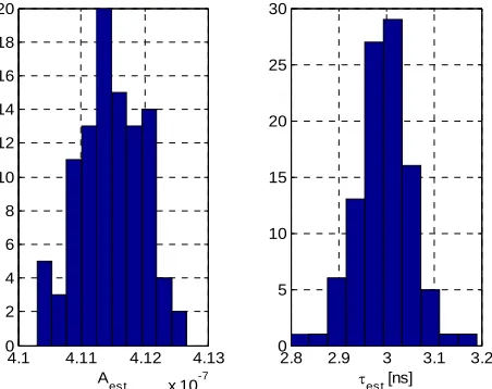
The Monte Carlo simulation results of the χ2 exhaus- tive search are shown in Figure 3 and Figure 4 The per-formance of the method is limited by the finite step size employed by the search algorithm. No obvious trend for the estimation error is observed.
5.2. Least-Square Exhaustive Search
The derivation of the weight matrix V (or the noise autocorrelation matrix R) requires precise knowledge of the impulse response of the detector front-end. The com- putation of the χ2 function in Eq. (2) also dictates N2 mul-tiplications for N samples when the off-diagonal entries of V are nonzero. In practice, the magnitude of the off-diagonal entries of R can be small relative to the main diagonal entries. In such cases, the V matrix can be well approximated by the identity matrix. Thus, Eq. (2) reduces to
Figure 2. The quadratic error surface of the χ2function in terms of A and τ.
4.1 4.11 4.12 4.13
x 10-7 0
2 4 6 8 10 12 14 16 18 20
A
est
2.8 2.9 3 3.1 3.2 0
5 10 15 20 25 30
[image:3.595.309.539.341.521.2]est [ns]
Figure 3. Histogram of 100 Monte Carlo runs for amplitude (left) and arrival time (right) estimation using the χ2 exhaustive search method. The standard deviation of the detector noise is set to 10% the peak value of the detector current pulse. The sample period T = 25 ns, A0 = 4.1134e-7, and τ0 = 3 ns.
-10 0 10
-1 -0.8 -0.6 -0.4 -0.2 0 0.2 0.4 0.6 0.8
1x 10
-9
delay [ns]
<A
es
t
- A
0
>
-10 0 10
-0.1 -0.08 -0.06 -0.04 -0.02 0 0.02 0.04 0.06 0.08 0.1
delay [ns]
<
es
t
-
0
> [n
s
]
2
-ES LS-ES
2
[image:3.595.58.285.542.704.2]-ES LS-ES
Figure 4. The χ2 versus the least-square search results of 1000 Monte Carlo runs: the mean estimation error and standard deviation for amplitude Aest (left) and arrival time
τest (right). τ0 = [−T/2, T/2]. Other simulation parameters are identical to those of Figure 3.
22 ,
i i i
A S Ag t
(3) This is identical to the least-square metrics to fit Nsamples to the known pulse shape g (t).
In our Monte Carlo simulation, the above argument is confirmed with a CR-RC2 pulse shaper. Again, an ex-haustive search is employed to determine the optimal fit of the five samples to g (t). The estimation errors for A
5.3. χ2 with First-Order Taylor Expansion
Taylor expansion can be performed on g(t) in the vicinity of τ = 0 to reduce the computation complexity of the χ2 function, i.e.,
i
i '
iAg t Ag t A g t (4) Where g'(t) is the first-order derivative of g(t). Thus,
2
1 2 ' 1 2
i i i ij j j
i j
S g g V S g g
'j
(5)whereα1 = A and α2 = Aτ.
Compared to Eq. (2), Eq. (5) defines a first-order ap-proximated quadratic error surface in terms of A and τ, which can be used to perform a search or to directly de- rive a closed-form analytical solution to the problem. The latter has been done in [10] and results are quoted as fol-lows
1 2 4 3 5
2 1 5 3
1
1
Q Q Q Q
Q Q Q Q
4
(6)
where
1
2
3
4
5
2
1 2 3
' '
'
'
i ij j ij
i ij j ij
i ij j ij
i ij j ij
i ij j ij
Q g V g
Q g V g
Q g V g
Q g V S
Q g V S
Q Q Q
(7)
5.4. Linear Optimal Filtering
A linear optimal filtering technique was proposed in [10] to minimize the computing effort involved in determina-tion of the amplitude and arrival time informadetermina-tion. The formulation of the optimal filter is quoted as follows
i i i
i i i
A u a S
A v b S
(8)
The coefficients of ai and bi are given as
a Vg Vg'
b Vg Vg' (9)
where λ = Q2/Δ, κ = −Q3/Δ, μ = Q3/Δ, ρ = −Q1/Δ, and Q and Δ are defined in Equation (7).
The advantage of this technique is that the filter tap
values are pre-calculated.Thus, the computation can be performed on the fly when data samples arrive, suitable for continuously operated detectors such as the proposed upgrade for ATLAS. It is also useful in resource-con- strainted implementation, e.g., FPGA or DSP, or latency- sensitive applications.
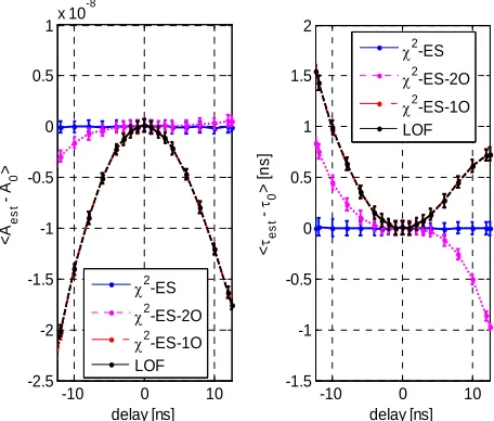
It can be shown that linear optimal filtering is equiva- lent to the χ2 method of first-order approximation [10]. The simulation results of both for A and τ are illustrated in Figure 5. It is interesting to note that the estimation error exhibits a quadratic dependence on τ as predicted by Eqs. (4) and (5) fortruncating the second- and higher- order terms in the Taylor expansion.
5.5. χ2 with Second-Order Taylor Expansion
The first-order Taylor expansion of the χ2 function leads to a rather large estimation error or bias when τ is large –−4.9% for amplitude and 12% for arrival time when τ
reaches ±T/2 in Figure 5,. One way to mitigate the large error is to iterate the series expansion and Equation (5) by re- calculating the g' and Q or, in the linear optimal filtering case, re-derive the filter tap values ai and bi and
iterate Equation (8). Simulation results are shown in Fig-ure 6 for linear optimal filtering with two iterations. The computing over- head in either case is significant. Another solution is to resort to a second-order Taylor expansion,
'
1 2
2
i i i '' i
Ag t Ag t A g t A g t (10)
Where g''(t) is the second-order derivative of g(t).
-10 0 10
-2.5 -2 -1.5 -1 -0.5 0 0.5
1x 10
-8
delay [ns]
<A
es
t
- A
0
>
-10 0 10
-1.5 -1 -0.5 0 0.5 1 1.5 2
delay [ns] <
es
t
-
0
> [
n
s
]
2
-ES
2
-ES-2O
2
-ES-1O LOF
2
-ES
2
-ES-2O
2
[image:4.595.310.538.471.665.2]-ES-1O LOF
Figure 5. The simulation results of 100 Monte Carlo runs for the first-order χ2 exhaustive search, linear optimal filtering, and second-order χ2 exhaustive search: the mean estimation error and standard deviation for amplitude Aest
(left) and arrival time τest (right). Simulation parameters
-10 0 10 -2.5
-2 -1.5 -1 -0.5 0 0.5
1x 10
-8
delay [ns]
<A
es
t
- A
0
>
-10 0 10
-0.2 0 0.2 0.4 0.6 0.8 1 1.2 1.4 1.6 1.8
delay [ns]
<
es
t
-
0
> [
n
s
]
1st iteration 2nd iteration
1st iteration 2nd iteration
Figure 6. The simulation results of 100 Monte Carlo runs for the linear optimal filtering case with two interations. Simulation parameters are identical to those of Figure 4.
The error surface of the second-order approximation can be similarly defined as of Equation (5). However, the nonlinearity of the second-order term excludes the possi-bility of a closed-form analytical solution. Thus, an ex-haustive search is performed instead and the simulation results are shown in Figure 5 as well. We note that the estimation error in this case exhibits a cubic dependence on τ as the truncation error in Equation (10) is dominated by the third order.
5.6. Gradient Descent Approach
As simulation results evidenced so far, the exhaustive search approach produces the best estimation accuracy at the cost of high computation complexity. To improve the efficiency of the search, a gradient-descent approach is devised. As illustrated in Figure 2, the bowl-shaped error surface of the χ2 function exhibits a global minimum. Starting from a random initial point on the surface, a search direction can be derived by comparing the value of the function at the current position to those offset by a step size away in both A and τ direction. The current po-sition is then advanced in the direction that minimizes the function value. The process is itereated until convergence at the bottom of the surface. Simulations for the gradient- descent approach were performed with four random starting point and the resulting search paths are plotted in
Figure 7. Comparing to the exhaustive search method in which the whole error surface is evaluated, the gradient- descent approach significantly reduces the computation involved. Table 1 compares the typical required number of iterations for the two cases.
6. Other Shapers
The amplitude and timing estimation techniques covered
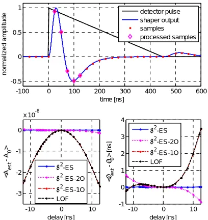
in Sec. 4 are also tested with CR-RC3 and CR2-RC2 pulse shapers. For the same 40-MHz sample rate, the peak of
g(t) falls in the middle between two samples in contrast to the case of the CR-RC2 shaper in which the peak is very close to a sample point. Figure 8 and Figure 9 plot
Figure 7. Simulated gradient-descent search paths for four random starting point on the error surface of the χ2function.
The x-axes are delay (in ns) and the y-axes are amplitude. Table 1. Effciency comparison between gradient-descent and exhaustive search methods.
Method Gradient Descent Exhaustive Search
Iterations 680* 603201
Computations per iteration
90 multiplications 72 additions 3 comparisons
30 multiplications 24 additions 1 comparison
*Averaged over different delay times.
-100 0 100 200 300 400 500 600
-0.2 0 0.2 0.4 0.6 0.8 1
time [ns]
nor
m
al
iz
ed am
pl
it
ude
-10 0 10
-3 -2 -1 0
x 10-8
delay [ns]
<A
es
t
-
A0
>
2
-ES
2
-ES-2O
2
-ES-1O LOF
-10 0 10
-1.5 -1 -0.5 0 0.5 1
delay [ns]
<
es
t
-
0
> [
n
s
]
2
-ES
2
-ES-2O
2
-ES-1O LOF detector pulse shaper output samples processed samples
REFERENCES
-100 0 100 200 300 400 500 600
-0.5 0 0.5 1
time [ns]
no
rm
al
ized
am
p
li
tud
e
-10 0 10
-3 -2 -1 0
x 10-8
delay [ns]
<A
es
t
-
A0
>
2-ES
2-ES-2O
2
-ES-1O LOF
-10 0 10
-1 0 1 2 3 4
delay [ns]
<
es
t
-
0
> [n
s
]
2
-ES
2-ES-2O
2-ES-1O
LOF detector pulse shaper output samples processed samples
[1] J. Wang, et al., “Nuclear Electronics,” 1st Edition, Atomic Energy Press, Beijing, 1983.
[2] T. R. Andeen, “Upgraded Readout Electronics for the ATLAS Liquid Argon Calorimeters at the High Luminos-ity LHC,” Journal of Physics Conference Series, Vol. 404, 2012, 012061.
[3] G. M. Haller, et al., “The LiquidArgon Calorimeter sys-tem for the SLC Large Detector,”IEEE Transactions on Nuclear Science, Vol. 36, No. 1, 1989, pp. 675-679.
doi:10.1109/23.34525
[4] ATLAS Collaboration, G. Aad, et al., “The ATLAS Ex-periment at the CERN Large Hadron Collider,” Journal of Instrumentation, Vol. 3, 2008, S08003.
[5] C. Collard, et al., “Prediction of Signal Amplitude and Shape for the ATLAS Electromagnetic Calorimeter,” ATLAS Notes, ATL-LARG-PUB-2007-010, Feb. 2008. [6] D. Banfi, et al., “Cell Response Equalization of the
[image:6.595.71.275.84.300.2]AT-LAS Electromagnetic Calorimeter without the Direct Knowledge of the Ionization Signals,” Journal of Instru-mentation, Vol. 1, Aug. 2006, P08001.
Figure 9. The simulation results of 100 Monte Carlo runs for CR2-RC2shaper. Simulation setupis identical to that of
Figure 4. Standard dev. bars are not shown for clarity. [7] ATLAS Collaboration, G. Aad, et al., “Drift Time Meas-urement in the ATLAS Liquid Argonelectro Magnetic Calorimeter Using Cosmic Muons,” European Physical Journal C, Vol. 70, No. 3, 2010, pp. 755-785.
the simulation results for the amplitude and timing esti-mation along with the input and output waveforms of the shaper. The skewed error curve reveals the asymmetry of the series expansion at off-peak sample points.
[8] M. Newcomer, “LAPAS: A SiGe Front End Prototype for the Upgraded ATLAS LAr Calorimeter,” Topical Work-shop on Electronics for Particle Physics, Paris, France, Sep. 21-25, 2009, pp. 132-135.
7. Conclusions
[9] H. Abreu, et al.,“Performance of the Electronic Readoutof the ATLAS Liquid Argon Calorimeters,”Journal of In-strumentation, Vol. 5, Sep. 2010, P09003.
Monte Carlo simulation results of various amplitude and timing estimation techniques for liquid ionization calo-rimeter signal processing are presented and compared. The tradeoff between computation complexity and esti-mation accuracy is studied. With the projected comput-ing power and cost scalcomput-ing for digital electronics in the future, the gradient-descent technique introduced in this paper can potentially become the leading approach for future nuclear/particle physics signal processing.
[10] W. E. Cleland and E. G. Stern, “Signal Processing Con-siderations for Liquid Ionization Calorimeters in a High Rate Environment,” Nuclear Instruments and Methods in Physics Research A, Vol. 338, 1994, pp. 467-497.
doi:10.1016/0168-9002(94)91332-3