Munich Personal RePEc Archive
Technical and scale efficiency in the
Italian Citrus Farming: A comparison
between Stochastic Frontier Analysis
(SFA) and Data Envelopment
Analysis(DEA) Models
Madau, Fabio A.
University of Sassari (Italy)
September 2012
Online at
https://mpra.ub.uni-muenchen.de/41403/
TECHNICAL AND SCALE EFFICIENCY IN THE ITALIAN CITRUS FARMING: A COMPARISON BETWEEN STOCHASTIC FRONTIER ANALYSIS (SFA) AND DATA ENVELOPMENT ANALYSIS (DEA) MODELS
Fabio A. Madau
University of Sassari, 07100
–
Sassari, Italy
ABSTRACT
This paper aims to estimate technical and scale efficiency in the Italian citrus farming. Estimation was carried out from two different approach: a non parametric and a parametric approach using a Data Envelopment Analysis (DEA) model and a Stochastic Frontier Analysis (SFA) model, respectively. Several studies have compared technical efficiency estimates derived from parametric and non parametric approaches, while a very small number of studies have aimed to compare scale efficiency obtained from different methodological approaches. This is one of the first attempts that aims to put on evidence possible difference in scale efficiency estimations in farming due to methods used. Empirical findings suggest that the greater portion of overall inefficiency in the sample might depend on producing below the production frontier than on operating under an inefficient scale. Furthermore, we found that the estimated technical efficiency from the SFA model is substantially at the same level of this estimated from DEA model, while the scale efficiency arisen from SFA is larger than this obtained from DEA analysis.
Keywords: Technical efficiency, Scale efficiency, Data Envelopment Analysis, Stochastic Frontier Analysis, Citrus farming,
J.E.L.: C13, Q12
______________________________________________________________________
1.INTRODUCTION
Since the Farrell’s (1957) seminar paper on efficiency estimation several parametric and non parametric procedures have been proposed in order to calculate efficiency and productivity of firms. However two main approaches have been mainly proposed in literature: the Stochastic Frontier Analysis (SFA) and the Data Enveopment Analysis (DEA). The former is a parametric technique originally and independently proposed by Aigner et al. (1977) and Meeusen and van der Broeck (1977) and the latter is a non parametric approach originally proposed by Charnes et al. (1978).
method and it cannot separate inefficiency component from noise. This approach also produces biased estimates in presence of measurement error and other statistical noise1. Several studies on comparing the two approaches have been proposed in literature (see
e.g. Gong and Sickles, 1992; Hjalmarsson et al. 1996; Sickles, 2005), also focusing attention on agriculture (Kalaitzandonakes and Dunn 1995; Sharma et al. 1997; Wadud and White, 2000; Minh and Long 2009). They have mostly investigated on differences between estimated technical efficiency scores and their distribution on the observed sample. Sharma et al. (1997) underlined that it is expected that the DEA efficiency scores would be less than those obtained under the specifications of stochastic frontier due to DEA method attributes any deviation of the data points from the frontier to inefficiency. However, empirical findings obtained from these studies confirm that the opposite may occur if the DEA frontier is fitted tightly to the sample data. Generally, the differences in the estimated results from two approaches could be mainly attributed to the different characteristics of the data, the choice of input and output variables, measurement and specification errors, as well as estimation procedures (Ruggiero 2007; Minh and Long 2009).
On the contrary, poor relevance has been given on comparison in measuring scale efficiency despite its important role in conditioning economic efficiency. Indeed, scale efficiency is a measure inherently relating to the returns to scale of a technology at any specific point of the production process (Førsund and Hjalmarsson 1979). It measures how close an observed plant is to the optimal scale, i.e. it describes the maximally attainable output for that input mix2 (Frisch, 1965).
In our opinion, more effort should be produced in comparing estimated scale efficiencies calculated from SFA and DEA approaches3. More attempts need to be done especially in agriculture due to the fact that a great number of papers have estimated scale efficiency in this sector but in most of these studies, the measure is calculated using a DEA model (Karagiannis and Sarris 2005; Bravo-Ureta et al., 2007). This is a relevant issue because differences in scale efficiencies interpretation and scale properties might derive form inherent differences between parametric and non parametric models. Therefore, it is expected to obtain some differences according to the methodology applied for estimating scale efficiencies in terms of scores and their distribution on the sample (Banker et al., 1986; Førsund. 1992).
Efficiencies measures arisen from DEA are technology invariant due to the DEA method of enveloping the data for construction the frontier and observed units at both ends of the size distribution may be identified as efficient simply for lack of other comparable units. It means that real economies of scale at large (or small) units will be difficult to detect and it may be an identification problem whether scale inefficiency of technically efficient units is real or due to the specification on variable returns to scale and the method of enveloping the data (Førsund. 1992). On the other hand, since the statistical theory is well developed for the parametric approaches, SFA allows us to make statistical inferences about estimated scale efficiency (Kumbhakar and Tsionas,
1
However, some authors have proposed models in which properties of SFA and DEA are integrated in order to overcame disadvantages of both methods (Ruggiero, 2004; Simar and Zeleneyuk, 2011).
2
This definition substantially corresponds to Banker’s (1984) concept of most productive scale size
(MPSS) in the DEA context.
3
2008). DEA generally does not permit to make it because any statements regarding the statistical properties of estimated efficiency measures including scale efficiencies can be formulated4. Furthermore, DEA and other deterministic models attributes any deviation of each observation from the frontier to inefficiency, while SFA models allow us to separate inefficiency component from noise.
According to Orea (2002) and Karagiannis and Sarris (2005), the approach followed for the DEA is hardly transferable using a SFA approach with flexible functional forms for the production frontier. DEA calculates scale efficiency by dividing the technical efficiency estimated under the hypothesis of constant return to scale and technical efficiency estimated imposing variable return to scale technology. In case of parametric approach, hypothesis that variable returns to scale technology is enveloped from the constant returns to scale technology is weak by a theoretical point of view. Indeed, there is nothing to guarantee that the variable returns to scale technology is enveloped from the constant returns to scale technology in the parametric context.
A model for estimating scale efficiency within a parametric flexible stochastic approach was proposed by Ray (1998). Following this methodology, a scale efficiency measure is obtained from the estimated parameters of the production frontier function under the variable returns to scale hypothesis and from the estimated scale elasticity. Ray’s (1998) model has the advantage of being easily tractable from the econometric point of view and being particularly suitable for a translog frontier function. In spite of these operational advantages, the model proposed by Ray (1998) has been scarcely adopted for estimating scale efficiency in agricultural studies.
The objective of this paper is to contribute in the existing literature providing a comparison between SFA and DEA approaches for estimating technical and scale efficiency. In particular both parametric and non parametric approaches were applied to estimate technical and scale efficiencies exhibited by the Italian citrus farming5. While several studies have compared technical efficiency estimates derived from parametric and non parametric approaches, this is one of the first attempts that aims to put on evidence possible difference in scale efficiency estimations in farming due to methods used, especially considering a stochastic specification of the production frontier in the parametric model. Regarding the parametric approach, a non-neutral production function model and the Ray (1998) model were applied to estimate technical and scale efficiency in the Italian citrus farming, respectively.
2.THE ITALIAN CITRUS FRUIT-GROWING SECTOR
Citrus fruit growing is one of the largest categories in the Italian vegetable and fruit sector. Since 2006, the value of production has amounted to more than 1 billion euro, accounting for about 10% of the total value of vegetables and fruits produced (Giuca 2008). Oranges comprise about 54% of citrus fruit production, whereas the contribution of lemons and tangerines to overall production (in terms of value) is equal to 17% and 19%, respectively.
4
As reported by Kumbhakar and Tsionas (2008), however some progress have been made into the DEA context in terms of bootstrapping and statistical properties of DEA findings.
5
The land area cultivated to citrus fruits corresponds to about 122,000 ha, while the number of farms is about 85,000 (Ismea 2008). Substantially, the farms are situated in the southern regions of Italy and, specifically, more than 70% of the farms and about 80% of cultivated land are located in only two regions: Sicily and Calabry. Since the early 1990s, however, land area covered by citrus fruits has decreased by about 30% (in 1990, it amounted to 184,000 ha) and the number of citrus farmers decreased by about 45% (about 170,000 in 1990). In this period, exports have slightly increased, while imports has grown sixfold (Giuca 2008).
Several reasons for this deterioration can be explored. First, the increasing competition in the world citrus fruit market has penalised Italian farmers because of structural and organisational problems that historically characterised the Italian citrus fruit sector. Specifically, Italian farms appear significantly small (on average, the area is 1.44 ha) and most of the citrus farms are located in less favourable areas where economic and productive alternatives are limited. Furthermore, despite the small size, many farms are fragmented in more plots of land, with evident implications on the ability to operate under efficient conditions.
These and other factors have contributed in the last few years to Italy’s declining competitiveness and efficiency in the world citrus fruit market. Structural constraints seem to negatively affect the performance of the Italian sector and inhibit economic development of citrus farming. The detection of technical and scale efficiencies can offer us more information about the nature of these problems. If significant technical and/or scale inefficiency were found, this would indicate that structural problems prevent farm expansion and the rational use of technical inputs. An analysis of the relationship between technical and scale (in)efficiency would allow us to determine direction priorities - technical efficiency or scale efficiency oriented measures - in order to improve overall efficiency in the farms.
3.METHODOLOGICAL BACKGROUND
Both for non parametric and parametric calculation of scale efficiency a preliminary step is estimating the frontier function and the correspondent measures of technical efficiency. As well-known, technical efficiency is defined as the measure of the ability of a firm to obtain the best production from a given set of inputs (output-increasing oriented), or as a measure of the ability to use the minimum feasible amount of inputs given a level of output (input-saving oriented) (Greene 1980; Atkinson and Cornwell 1994)6. This section illustrates how technical and scale efficiency output-oriented measures can be obtained from the DEA and the SFA models7.
3.1 Non parametric estimation: Data Envelopment Analysis (DEA)
Data Envelopment Analysis (DEA) is a non parametric approach to estimate efficiency originally proposed by Charnes et al. (1978) and based on the Farrell’s model (1957). DEA consents the estimation of efficiency in multi-output situations and without
6
When firm operates in a constant returns to scale area the input and output-oriented measures coincide (Fare and Lovell 1978).
7
assuming a priori functional form for frontier production (Roland and Vassdal, 2000). Therefore DEA assumes that the production function is unknown and solving a linear programming problem it calculates efficiency by comparing each production unit against all other units. The best practice frontier is represented by a piecewise linear envelopment surface. Therefore, TE scores arisen from DEA are invariant to technology, because obtained trough comparisons among an observation and each others and not with respect to an estimated frontier.
The discussion on DEA presented here is brief and concerns the output-oriented
Constant Return to Scale (CRS) DEA and Variable Return to Scale (VRS) DEA. The
output-oriented CRS DEA model for a single output is described below. TE is derived solving the following linear programming model (Ali and Seiford 1993):
max q,l qi
subject to - -s 0
1 =
å
= i in
j ljyj q y
ki k n
j jxkj+e = x
å
=1llj ³ 0; s³ 0; ek³ 0 (1)
where qi is the proportional increase in output possible for the i-th DMU (Decision Making Unit that in this study is a farm), lj is an N´1 vector of weights relative to efficient DMUs, s is the output slack; and ek is the k-th input slack. Banker et al. (1984)
suggest to adapting the CRS DEA model in order to account for a variable returns to scale situation. Adding the convexity constraint N1’l = 1, the model can be modified into VRS DEA8.
The proportional increase in output which is possible is accomplished when output slack, s, becomes zero. A DMU results efficient when the values of θ and li are equal to
1; and lj = 0. On the contrary, a DMU is inefficient when θ > 1, li = 0; and lj ≠ 0. Solving (1) we can obtain a measure of TE that reflects “distance” between the observed and optimal output production for a certain inputs bundle:
TEi =
*
i Y
i Y
=
i
q 1
0 ≤ TEi≤ 1 (2)
where Yi and Yi*are the observed and maximum possible (optimal) output, respectively. A measure of scale efficiency (SE) can be obtained by comparing TECRS and TEVRS scores. Any difference between the two TE scores indicates there is scale inefficiency that limits achievement of an optimal (constant) scale:
CRS i
TE = TEVRSi * SEi (3)
Therefore, it can be calculated as (Coelli 1996a):
8
SEi = VRS i CRS i
TE TE
0 ≤ SEi≤ 1 (4)
where SEi = 1 indicates full scale efficiency and SEi < 1 indicates presence of scale
inefficiency.
However, a shortcoming of the SE score is that it does not indicate if a farm is operating under increasing or decreasing return to scale. This is resolvable by simply imposing a
non-increasing return of scale (NIRS) condition in the DEA model, i.e. changing the convexity constraint N1’l = 1 of the DEA VRS model into N1’l ≤ 1. If TENIRS and TEVRS are unequal, then farms operate under increasing return to scale (IRS); if they are equal a decreasing return to scale (DRS) exists.
3.2 Parametric Estimation: Stochastic Frontier Analysis (SFA)
SFA was originally and independently proposed by Aigner et al. (1977) and Meeusen and van der Broeck (1977). In these models, the production frontier is specified which defines output as a stochastic function of a given set of inputs. The presence of stochastic elements makes the models less vulnerable to the influence of outliers than with deterministic frontier models. It concerns that the error term e may be separated in two terms: a random error and a random variable explanatory of inefficiency effects:
yit = f (xit, t; ß) · exp e (5a)
e = (vit - uit) i = 1,2,….N t = 1,2,….T (5b)
where yit denotes the level of output for the i-th observation at year t; xit is the row
vector of inputs; t is the time index, ß is the vector of parameters to be estimated; f (•) is a suitable functional form for the frontier (generally Translog or Cobb-Douglas); vit is a
symmetric random error assumed to account for measurement error and other factors not under the control of the firm; and uit is an asymmetric non-negative error term
assumed to account for technical inefficiency in production.
The vi’s are usually assumed to be independent and identically distributed N (0, sv 2
) random errors, independent of the uit’s that are assumed to be independent and
identically distributed and with truncation (at zero) of the normal distribution ½N (0,
su 2
)½. The Maximum Likelihood Estimation (MLE) of (5) allows us to estimate the vector ß and the variance parameters s2=su2 +sv2 and g = su / sv; where 0 ≤g ≤ 1. The
TE measure is obtained by the ratio of yitto the maximum achievable level of output:
TE = *
y yit
= exp (- uit) (6)
where y* is the output that lies on the frontier. Furthermore, assuming a semi-normal distribution for uit and according to Jondrow et al. (1982), the degree of technical
efficiency of each firm could be estimated.
technical efficiency with some explanatory variables (Pitt and Lee 1981; Kalirajan 1982; Parikh and Shah 1994).
One-stage SFA models in which the inefficiency effects (ui) are expressed as a function
of a vector of observable explanatory variables were proposed by Kumbhakar et al.
(1991), Reisfschneider and Stevenson (1991), Huang and Liu (1994). In this model, all parameters – frontier production and inefficiency effects – are estimated simultaneously. This approach was adapted by Battese and Coelli (1995) to account for panel data. They proposed an one-stage approach where the functional relationship between inefficiency effects and the firm-specific factors is directly incorporated into the MLE. The inefficiency term uit has a truncated (at zero) normal distribution with
mean mit:
uit= mit+ Wit (7a)
where Witis a random error term which is assumed to be independently distributed, with
a truncated (at -mit) normal distribution with mean zero and variance σ2 (i.e. Wit≥ - zit
suchthat uit is non-negative).
The mean mit is defined as:
mit = Z (zit, d) i = 1,2,….N t = 1,2,….T (7b)
where Z is the vector (Mx1) of the zit firm-specific inefficiency variables of
inefficiency; and d is the (1xM) vector of unknown coefficients associated with zit. So
we are able to estimate inefficiency effects arisen from the zit explanatory variables9.
Orea (2002) argues that the non parametric approach difficultly can be directly transferred into a parametric approach in order to calculate scale efficiency. Indeed when parametric approach is used, hypothesis that VRS technology is enveloped from CRS technology is weak by a theoretical point of view.
As mentioned above, Ray (1998) proposed a model in which scale efficiency can be calculated from the estimated parameters of the production frontier and from scale elasticity estimations. For a translog frontier function:
ln yit = β0 + ln ln
-2 1
ln ( )
1 1 1 it it l k kit jit jk n j n j jit
j
x
βx
x
v
u
β +
å
å
× +å
= =
= (8)
and assuming an output-oriented approach for the technical efficiency estimation, scale elasticity at farm-specific input bundle is equal to:
å
å
= = ÷ ø ö ç èæ + +
= n 1 j l 1 k
Eit bj bjkxkit bjit
(9)
Remanding to Ray (1998) for a more detailed description of the methodology, it follows that the output-oriented scale efficiency (SEO) corresponds to:
9
(
)
ú û ù ê ë é = b 2 E -1 exp SE 2 it O it (10) where:å å
= = = n j l k jk 1 1 b b (11)with ß that is assumed to be negative definite as to guarantee that 0 < SEOit ≤ 1
10
.
This output-oriented scale efficiency measures the role of scale in conditioning technical efficiency. Scale efficiency reflects the relative output expansion by producing at optimal scale on the frontier for the observed factor proportions of a firm whose technical inefficiency has been eliminated (Karagiannis and Sarris 2005). In other terms, following the Frisch’s definition, scale efficiency measures the distance to full efficient scale after moving a production unit to the frontier in the vertical direction. As reported by Ray (1998), scale efficiency (10) and scale elasticity (9) are both equal to one only at an MPSS, i.e. where constant returns to scale prevails. Elsewhere they differ and SE is <1 irrespective of whether Eit is greater than or less than unity. It means
that the magnitude of scale elasticity reveals nothing about the level of SE at the points different by the MPSS.
On the basis of the definition of scale efficiency measured by (10), the sub-optimal scale is associated with increasing returns to scale. When Eit > 0 (increasing returns to
scale) then SE increases with an increase in output and the optimal scale should be reached expanding the observed output level. Vice versa, output should be contracted to reach the optimal scale when a plan operates in a decreasing returns to scale (supra-optimal) area (Eit < 0)11.
In order to explain scale efficiency differentials among plans, Karagiannis and Sarris (2005) used a two-stage approach. At the first stage, SEs are estimated using the formula (10) and successively, at the second stage, the SE scores are regressed against a set of explanatory variables. Following the procedure proposed by Reinhard et al.
(2002), these authors in the second stage used a MLE technique to estimate this stochastic frontier regression model:
ln O it
SE = mit+ εit with (12a)
mit = Z (zit, r) and (12b)
eit = (
* it
v -u*it) i = 1,2,….N t = 1,2,….T (12c)
where zit represents the same set of variables used in the inefficiency model (9), r are
the parameters to be estimated, εit is the error term composed by vit* that represents the
10
Negative definiteness of β is a sufficient but not necessary condition (Ray, 1998).
11
statistical noise (independently and identically distributed with N (0, 2 * v
s ) random variable truncated at -mit) and by u*it that represents the conditional scale inefficiency remaining even after variation in the zit has been accounted for (uit* ~N (-mit,
2 * u
s )). The two-stage approach in the SFA models has been criticized by several authors because it is inconsistent in it’s assumption regarding independence of the inefficiency effects (Battese and Coelli 1995; Kumbhakar and Lovell 2000). With specific reference to technical efficiency, the rationale underlying is that the specification of the regression of the second stage - in which the estimated technical efficiency scores are assumed to have a functional relationship with the explanatory variables - conflicts with the assumption that ui’s are independently and identically distributed (TE is the dependent
variable in the second stage procedure).
However, as underlined by Reinhard et al. (2002), a two-stage procedure can consistently be used as long as the efficiency scores are calculated from the first-stage parameter estimates, instead of being estimated econometrically at the first stage. In the case of the procedure illustrated above for computing scale efficiency effects, no such assumption is made with respect to the dependent variable SE because SE scores are obtained from the parameter estimates and the estimated values of scale elasticity. Thus, Reinhard et al. (2002) recommended application of the two-stage procedure for estimating scale efficiency effects.
4.DATA AND THE EMPIRICAL MODELS
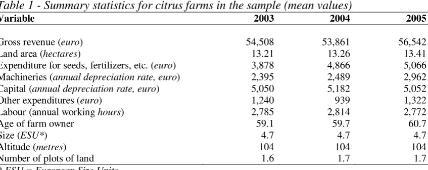
Data were collected on a balanced panel data of 107 Italian citrus farms. All the selected farms participated in the official Farm Accountancy Data Network (FADN) during the period 2003-2005 and they are specialized in citrus fruit-growing (more then 2/3 of farm gross revenue arises from citrus production). Farms with less than two European Size Units (ESU) were excluded from the sample12. Therefore, both non parametric and parametric analyses are based on a total of 321 observations (see Table 1 for summary statistics about farms).
4.1DEA model
We applied both CRS and VRS DEA models in order to calculate scale efficiency. Estimation of technical and scale efficiency was carried out performing separated analysis for each considered year.
The dependent variable (Y) represents the output and it is measured in terms of gross revenue from the i-th farm. The aggregate inputs, included as variables of the production function, are 1) X1 the total land area (hectares) devoted to citrus
fruit-growing by each farm; 2) X2 the expenditure (euro) for seeds, fertilizers, water and other
variable inputs used in the citrus fruits-growing; 3) X3 the value (euro) of machineries
used in the farm; 4) X4 the value (euro) of capital (amount of fixed inputs such as
buildings and irrigation plant, except for machineries); 5) X5 the expenditure (euro) for
other inputs, consisting in fuel, electric power, interest payments, taxes, etc.; 6) X6 the
total amount (annual working hours) of labour (including family and hired workers);
12
Regarding the machineries and capital variables, they were measured in terms of annual depreciation rate so to have a measure of annual utilization, on average, of the capital stock13. All variables measured in monetary terms were converted into 2003 constant euro value.
Table 1 - Summary statistics for citrus farms in the sample (mean values)
Variable 2003 2004 2005
Gross revenue (euro) 54,508 53,861 56,542 Land area (hectares) 13.21 13.26 13.41 Expenditure for seeds, fertilizers, etc. (euro) 3,878 4,866 5,066 Machineries (annual depreciation rate, euro) 2,395 2,489 2,962 Capital (annual depreciation rate, euro) 5,050 5,182 5,052 Other expenditures (euro) 1,240 939 1,322 Labour (annual working hours) 2,785 2,814 2,772 Age of farm owner 59.1 59.7 60.7 Size (ESU*) 4.7 4.7 4.7 Altitude (metres) 104 104 104 Number of plots of land 1.6 1.7 1.7
* ESU = European Size Units
Furthermore, a set of explanatory variables of efficiency were selected in order to evaluate their effect on technical and scale efficiency. More precisely, individual estimated technical and scale efficiency were regressed to: 1) Z1 the age of the farm
owner; 2) Z2a dummy variable that reflects the size of the farm measured in terms of
ESU that can assume a value involved from 3 to 714; 3) Z3the variable altitude that
reflects the average altitude (in metres) by each farm; 4) Z4the number of plots of land
in which farm is fragmentized; Z5 a dummy variable that reflects the placement (or not)
of each farm in a Less-favoured area such as defined by the EEC Directive 75/268 (0 = Less-Favoured zone; 1 = non Less-favoured zone); Z6-Z11 that represent a set of dummy
variables indicating the regional location of farms (Rcam = Campany; Rcal = Calabria;
Rapu = Apulia; Rbas = Basilicata; Rsic = Sicily; Rsar = Sardinia).
Variables such as age of farmers, farm size, and regional location have been widely used in the efficiency analyses applied to agriculture. The first is generally used as a proxy of farmer skills, experience, and learning-by-doing (the rationale is that the expected level of efficiency increases with experience). The second was implemented to evaluate the role of farm economic size in conditioning efficiency (a positive sign is expected, i.e. efficiency tends to increase in larger farms). The third serves to estimate the presence of territorial and geographic variability that may affect efficiency.
Altitude and location in a less-favoured area are variables used in some efficiency analysis to account for geoclimatic and socioeconomic heterogeneities (Karagiannis and Sarris 2005; Madau 2007). On the other hand, the number of lots has not been a variable generally employed in the efficiency analyses in agriculture. But, in our opinion and as highlighted above, it could be significant in conditioning both farm technical and scale efficiencies in the Italian citrus farming. Indeed, the subdivision of the farm land area
13
As underlined by Madau (2008), value of capital goods is estimated in different ways into the efficiency analyses. Some authors have considered the total amount of value, whereas other authors have expressed capital in terms of annual capacity utilization. In this case, the capital measure depends on the adopted criteria for calculate capacity utilization.
14
into more plots of land could be an obstacle toward achieving full (technical and scale) efficiency on the part of farmers.
4.2SFA model
We assumed a Translog functional form as frontier technology specification for the citrus farms. The adopted model corresponds to the Huang and Liu (1994) non-neutral production function model applied on panel data, which assumes that technical efficiency depends on both the method of application of inputs and the intensity of input use (Karagiannis and Tzouvelekas 2005)15. It means that the inefficiency term uit
explained by (7) is equal to:
uit= d0 +
å
=
N
i 1
dit zi +
å
=
M
m 1
dm ln xmit +Wit i = 1,2,….N t = 1,2,….T (13)
The Translog stochastic function production model is specified as formula (8) and involves seven variables: the variables X1-X6 correspond to the same bundle of inputs
selected for the DEA model and X7 is a variable that represents the time (year) and it can
assume value equal to 1 (2003), 2 (2004) or 3 (2005).
In the inefficiency model (13) we found the same set of explanatory variables used for the DEA model. In addition, according to the non-neutral model proposed by Huang and Liu (1994), (in)efficiency is expected to depend by the inputs used in the production. Therefore, the same pool of variables (included time) used to describe the frontier function production (xit) were included in the inefficiency model.
Finally, applying the second-stage regression (12), scale efficiency effects were calculated using the same bundle of variables used for the technical efficiency effects model, with the exception of inputs that describe the frontier production.
5.ANALYTICAL FINDINGS
5.1 Estimated results from non parametric approach
Technical efficiency scores arisen by application of the DEA model were estimated using the DEAP 2.1 program created by Coelli (1996a).
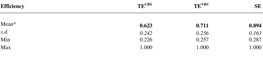
Results indicate that output-efficiency technical efficiency obtained for the CRS and VRS frontiers are, on average, equal to 0.623 and 0.711, respectively (Table 2). These measures were calculated as averages on the triennial period of observation (2003-2005). Considering the latter measure – so called “pure efficiency” because devoid of scale efficiency effects – and since technical efficiency scores are calculated as an output-oriented measure, the results imply that citrus fruits-growing farmers would be able to increase output by about 30% using their disposable resources more effectively (at the present state of technology).
Scale efficiency is calculated applying formula (4). The mean scale efficiency for the Italian citrus fruits producers in Italy is equal to 0.894. It means that adjusting the scale of the operation, citrus farms could improve their efficiency by 10.6%.
15
Imposing the NIRS condition, we found that the most of the farms exhibit an increasing returns to scale (Table 3). Of the 107 farms, 71 (66.3%) show increasing (sub-optimal) returns to scale, 22 (20.6%) show constant (optimal) returns to scale, and 14 (13.1) show decreasing (supra-optimal) returns to scale. Therefore, this implies that scale inefficiency is mainly due to the farms operating under a sub-optimal scale, - i.e. farms where their output levels are lower than optimal levels and they should be expanded to reach the optimal scale. It was found that typology of returns to scale do not vary in each farms during the time of observation.
Tab.2 – Estimated technical efficiency and scale efficiency using DEA
Efficiency TECRS TEVRS SE
Mean* 0.623 0.711 0.894
s.d. 0.242 0.256 0.163
Min 0.226 0.257 0.287
Max 1.000 1.000 1.000
* calculated on the basis of a triennial period
[image:13.595.84.513.225.322.2]In the most of sub-optimal scale farms, scale efficiency is sensitively low (the average SE in this group is less than 0.700). On the contrary, supra-optimal scale farms appear more efficient, in terms of ability to operate under an adequate scale (mean SE equal to 0.934). Both TE and SE scores vary substantially across farms. To explain some of these variations, the efficiency scores were regressed on the farm-level characteristics. A Tobit regression model was used, since the efficiencies vary from zero to unity.
Table 3 – Scale efficiency and returns to scale from DEA
Observations Scale Efficiency
n. %
Total sample (mean) 321 100 0.894
Supra-optimal scale 42 13.1 0.934
Optimal scale 66 20.6 1.000
Sub-optimal scale 213 66.3 0.692
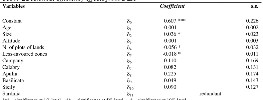
Age of farmer is negatively related to technical efficiency, but the estimated coefficient is not statistically significant (Table 4). Farm size is positively related to efficiency level. The results indicate that improvement of technical efficiency depends, among the others, on citrus farms attaining an adequate size (magnitude is equal to 0.036). Altitude slightly affects technical efficiency, while, as expected, the number of lots is negatively correlated to technical efficiency.
The findings imply that technical efficiency tends to decrease in the case of partitioning farms in more plots. The magnitude of this effect is 0.056, indicating that the presence of a plurality of lots affects sensitively efficiency from a technical point of view. Furthermore, farms situated in less-favoured areas tend to be more inefficient than those located in normal zones (magnitude is equal to -0.018). Finally, the fact that all the
Table 5 shows results on relationship between scale efficiency and possible sources of inefficiency. Age of farmers is negatively related to scale efficiency, even if magnitude is not sizeable (-0.003). It implies that citrus farms managed by younger farmers should be more scale efficient than farms managed by older farmers. Farm size might positively affect scale efficiency. It is the factor that contributes the most to conditioning scale efficiency (magnitude is equal to 0.042). This suggests that large-sized farms tend to have higher scale efficiency than small-scale farms. Altitude and location in a less-favoured area are not significant variables by a statistical point of view. On the contrary, the number of plots of land represents the second most important factor in the order of importance that affects scale efficiency (-0.040). The consistent negative sign of the estimated coefficient indicates that in-farm land fragmentation might be a relevant structural constraint to achieving an adequate scale efficiency by part of citrus farmers.
Tab.4 – Technical efficiency effects from DEA
Variables Coefficient s.e.
Constant d0 0.607 *** 0.226
Age d1 -0.001 0.002
Size d2 0.036 * 0.023
Altitude d3 -0.001 0.003
N. of plots of lands d4 -0.056 * 0.032
Less-favoured zones d5 -0.018 * 0.011
Campany d6 0.110 0.169
Calabry d7 0.082 0.131
Apulia d8 0.225 0.174
Basilicata d9 0.049 0.143
Sicily d10 0.090 0.127
Sardinia d11 redundant
*** = significance at 1% level ** = significance at 5% level * = significance at 10% level
Tab.5 – Scale efficiency effects from DEA
Variables Coefficient s.e.
Constant d0 0.756 *** 0.145
Age d1 -0.003 ** 0.001
Size d2 0.042 ** 0.020
Altitude d3 -0.001 0.002
N. of plots of lands d4 -0.040 ** 0.018
Less-favoured zones d5 0.005 0 012
Campany d6 0.269 * 0.167
Calabry d7 -0.002 0.089
Apulia d8 -0.045 0.102
Basilicata d9 -0.093 * 0.049
Sicily d10 -0.179 ** 0.082
Sardinia d11 redundant
*** = significance at 1% level ** = significance at 5% level * = significance at 10% level
Finally, the findings show that there are statistically significant differences in scale efficiency between farms located in different geographical regions of Italy, implying that location sensitively influences scale efficiency.
5.2 Estimated results from parametric approach
Parameters for the function and inefficiency model were estimated simultaneously. ML estimation was obtained using the computer program FRONTIER 4.1, created by Coelli (1996b). ML estimates for the preferred frontier model were obtained after testing various null hypotheses in order to evaluate suitability and significance of the adopted model.As testing procedure we adopted the Generalised likelihood-ratio test, which allows us to evaluate a restricted model with respect to the adopted model (Bohrnstedt and Knoke, 1994)16.
The test was applied in order to estimate the more suitable to the data functional form o the frontier (Transolg or Cobb-Douglas specification; non-neutral or neutral specification), presence of inefficiency effects, nature of inefficiency effects, presence of an intercept in the inefficiency model, presence of farm-specific factors, presence of regional effects and, finally, presence of Age and Altitude effects (because of poor estimated statistical significance).
Table 6 reports the results of these t-tests and in the light of these the model was estimated to obtain the preferred form. MLE for the more appropriate model are shown, as reported above, in the Table 7.
Since the Translog function takes into account also interaction among involved inputs, the production elasticities were computed using the traditional formula for the estimation of the elasticity of the mean output with respect to the k-th input (except for the time variable):
) ln(
) ( ln
k
x Y E
¶ 
= 2
k j
å
¹ +
+ kk ki kj ji
k b x b x
b
(14)
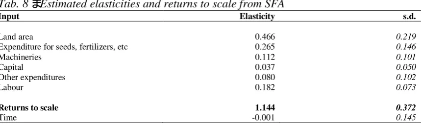
Application of (14) indicates that, at the point of approximation, the estimated function satisfies the monotonicity (all parameters show a positive sign) and diminishing marginal productivities (magnitude is lower than unity for each parameter) properties (Table 8).
The estimated production elasticities suggest that land is the foremost important input followed by expenditure for seeds and other technical inputs, labour, and machineries. It means that enlargement of the land area would affect significantly farm productivity. Specifically holding all other inputs constant, an increase of 1% in land area would result in a 0.47% increase in output. According to other research findings, the high elasticity of the land area is not surprising in presence of small size farms because this factor could be considered a quasi-fixed input (Alvarez and Arias 2004; Madau 2007). Except for land area, these findings suggest that production of Italian citrus farms is sensitively elastic with respect to these factors, which should allow farmers to easily vary their own use level in the short run - elasticity of seeds (and other technical inputs) and labour is equal to 0.27 and 0.18, respectively - while the other quasi-fixed inputs (capital and machinery) affect productivity less (elasticity equal to 0.04 and 0.11,
16
respectively). The time variable shows a negative sign, but the magnitude is not relevant, implying that time does not significantly affect production.
Table 6 – Hypothesis testing for the adopted model for SFA
Restrictions Model L(H0) l d.f. 2
95 . 0
c Decision
None Translog, non neutral -89.81
H0 : δm= 0 Neutral -100.18 20.74 6 12.59 Rejected
H0 : bij= 0 Cobb-Douglas -168.34 157.06 21 32.67 Rejected
H0 : g = d0; dr;dm = 0 No inefficiency effects -120.45 61.28 6 11.91* Rejected
H0 : g = d0;dm = 0 No stochastic effects -101.80 23.98 9 19.92* Rejected
H0 : d0= 0 No intercept -90.44 1.26 1 3.84 Not rejected
H0 : dr;dm = 0 No firm-specific factors -118.76 57.90 11 19.68 Rejected
H0 : d6….d11 = 0 No Regional effects -94.88 10.14 6 12.59 Not rejected
H0 : d1; d3 = 0 No Age and Altitude effects -92.65 5.68 2 5.99 Not rejected
* Critical values with asterisk are taken from Kodde and Palm (1986). For these variables the statistic l is distributed following a mixed c2 distribution.
Returns to scale were found to be clearly increasing (1.144). Therefore, the hypothesis of constant returns to scale is rejected. It means that citrus farmers should enlarge the production scale by about 14%, on average, in order to adequately expand productivity, given their disposable resources.
As to the estimated technical efficiencies, the analysis reveals that, on average, citrus farms are 71% efficient in using their technology (Table 7). Since technical efficiency scores are calculated as an output-oriented measure, the results imply that farmers would be able to increase output by about 30% using their disposable resources more effectively (at the present state of technology).
The estimated ratio-parameter g is significant (for α = 0.01) and it indicates that differences in technical efficiency among farms is relevant in explaining output variability in citrus fruits-growing (1/3 of the variability on the whole). Estimation of this parameter γ* suggests that about 58% of the general differential between observed and best-practice output is due to the existing difference in efficiency among farmers. Therefore, technical efficiency might play a crucial role into the factors affecting productivity in the citrus farming.
Empirical findings concerning the sources of efficiency differentials among farms are presented in Table 7. Farm size is positively related to efficiency level. The results indicate that improvement of technical efficiency strongly depends on citrus farms attaining an adequate size (magnitude is equal to 0.495). Specifically, farm size increase should affect positively both productivity (returns to scale more than unity) and efficiency (negative sign of Size variable).
As expected, the number of lots is negatively correlated to technical efficiency, implying that technical efficiency tends to decrease in the case of partitioning farms in more plots, also if the magnitude of this effect is low (0.014) Finally, farms situated in less-favoured areas tend to be more inefficient than those located in normal zones (0.012)17.
17
Tab. 7a – ML Estimates for SFA parameters and for TE (preferred model) - continue
Variables Parameter Coefficient s.e
FRONTIER MODEL
Constant b0 -0.608 0.139
Land Area b1 -1.827 0.422
Expenditure for seeds, fertilizers, etc. b2 1.515 0.463
Machineries b3 1.662 0.378
Capital b4 -0.526 0.453
Other expenditures b5 0.193 0.287
Labour b6 0.576 0.569
Year bT -1.697 0.696
(Land Area) x (Land Area) b11 0.052 0.037
(Land Area) x (V. expenditure) b12 0.102 0.038
(Land Area) x (Machineries) b13 0.085 0.028
(Land Area) x (Capital) b14 0.021 0.036
(Land Area) x (O. expenditures) b15 0.010 0.035
(Land Area) x (Labour) b16 0.060 0.060
(Land Area) x (Year) b1T -0.111 0.053
(V. expenditure) x (V. expenditure) b22 0.032 0.031
(V. expenditure) x (Machineries) b23 0.016 0.026
(V. expenditure) x (Capital) b24 -0.053 0.037
(V. expenditure) x (O. expenditures) b25 0.099 0.033
(V. expenditure) x (Labour) b26 -0.328 0.069
(V. expenditure) x (Year) b2T -0.011 0.055
(Machineries) x (Machineries) b33 0.074 0.017
(Machineries) x (Capital) b34 -0.088 0.033
(Machineries) x (O. expenditures) b35 -0.125 0.035
(Machineries) x (Labour) b36 -0.198 0.051
(Machineries) x (Year) b3T -0.020 0.035
(Capital) x (Capital) b44 0.030 0.024
(Capital) x (O. expenditures) b45 0.085 0.024
(Capital) x (Labour) b46 0.046 0.058
(Capital) x (Year) b4T 0.076 0.051
(O. expenditures) x (O. expenditures) b55 0.029 0.021
(O. expenditures) x (Labour) b56 -0.137 0.072
(O. expenditures) x (Year) b5T 0.089 0.048
(Labour) x (Labour) b66 0.228 0.076
(Labour) x (Year) b6T 0.141 0.065
(Year) x (Year) bTT 0.026 0.076
INEFFICIENCY MODEL
Constant d0 - -
Age d1 -
Size d2 -0.495 0.087
Altitude d3 - -
Number of plots of land d4 0.014 0.031
Less-favoured zones d5 0.012 0.010
Campany d6 - -
Calabria d7 - -
Apulia d8 - -
Basilicata d9 - -
Sicily d10 - -
Sardinia d11 - -
Land Area dSUP -0.679 0.147
Expenditure for seeds, fertilizers, etc. dSV 0.359 0.105
Machineries dQM -0.043 0.062
Capital dQC 0.068 0.110
Other expenditures dAS 0.319 0.149
Labour dLAV -0.740 0.214
Tab. 7b – ML Estimates for SFA parameters and for TE (preferred model)
Variables Parameter Coefficient s.d.
VARIANCE PARAMETERS
s2
s2 0.127 0.016
g g 0.333 0.131
g* g* 0.579
Log-likelihood function -92.66
TECHNICAL EFFICIENCY
Mean 0.710
s.d 0.266
Maximum 1.000
Minimum 0.060
Regarding the relationship between technical efficiency and technical inputs, ML estimation shows that all inputs have a significant part to play in determining efficiency (Table 7). Land area, labour, and machinery carry a negative sign, implying that an increase in each variable positively affects technical efficiency.
Finally, the empirical findings suggest that farmers tend to become less efficient over time even if the magnitude is really low (0.091)18.
Tab. 8 – Estimated elasticities and returns to scale from SFA
Input Elasticity s.d.
Land area 0.466 0.219
Expenditure for seeds, fertilizers, etc 0.265 0.146
Machineries 0.112 0.101
Capital 0.037 0.050
Other expenditures 0.080 0.102
Labour 0.182 0.073
Returns to scale 1.144 0.372
Time -0.001 0.145
[image:18.595.87.518.358.485.2]Scale elasticities and scale efficiencies were estimated applying formulas (9) and (10). Table 9 shows that the average scale efficiency is 81.8%. It implies that observed farms could have further increased their output by about 18% if they had adopted an optimal scale. Results also indicate that about 80% of the observations exhibit increasing returns to scale. They operate under a suboptimal scale, i.e., their output levels are lower than optimal levels and they should be expanded to reach the optimal scale. In these farms, scale efficiency is sensitively lower than the average (77.5%) and the average scale elasticity is abundantly upper than unity (1.237).
On the other hand, only about 6% of the observations are characterised by operating under an optimal scale, while about 15% of the panel reveals decreasing returns to scale. The relationship between scale efficiency and farm size seems to be confirmed by analytical results on the scale efficiency effects (see Table 11 below). These were obtained from application of (12) to the estimated data. The original proposed model – the second-stage regression of the scale efficiency scores to the variables described
18
above - was tested using the Generalised likelihood-ratio test procedure in order to evaluate if a restricted model is preferable. Specifically three tests were applied concerning hypotheses on presence of intercept in the inefficiency effects, role of the regional areas in conditioning the farm scale inefficiency and presence of the Less-favoured area parameter, respectively. On the basis of the t-test results (reported in Table 10), we estimated the preferred model that is different from the proposed one for the absence of the intercept and the Less-favoured area variable. Estimated findings of scale inefficiency effects are reported in Table 11.
Tab. 9 – Estimated scale efficiency and scale elasticity from SFA
Observations Scale efficiency Scale elasticity
n. %
Total sample (mean) 321 100 0.818 1.144
s.d 0.213 0.416
Maximum 1.000 1.588
Minimum 0.012 0.662
Supra-optimal scale 47 14.7 0.978 0.897
Optimal scale 19 5.9 1.000 1.000
Sub-optimal scale 225 79.4 0.775 1.237
Table 10 – Hypothesis testing for the scale efficiency effects model from SFA
Restrictions Model L(H0) l d.f. 2
95 . 0
c Decision
None Translog, non neutral 123.92
H0 : d0= 0 No intercept 123.92 0.01 1 3.84 Not rejected
H0 : d6….d11 = 0 No Regional effects 114.71 18.42 6 12.59 Rejected
H0 : d5 = 0 No Less-favoured area effects 112.88 2.08 1 3.84 Not rejected
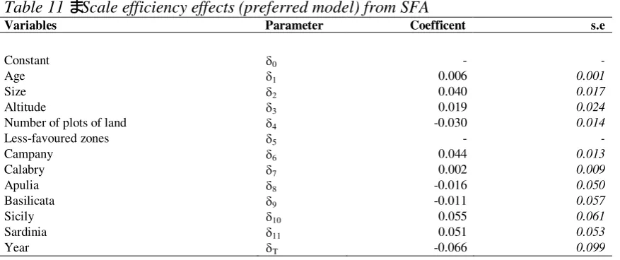
Farm size is the factor that contributes the most to conditioning positively scale efficiency (magnitude is equal to 0.040). This suggests that large-sized farms tend to have, as expected, higher scale efficiency than small-scale farms.
Table 11 – Scale efficiency effects (preferred model) from SFA
Variables Parameter Coefficent s.e
Constant d0 - -
Age d1 0.006 0.001
Size d2 0.040 0.017
Altitude d3 0.019 0.024
Number of plots of land d4 -0.030 0.014
Less-favoured zones d5 - -
Campany d6 0.044 0.013
Calabry d7 0.002 0.009
Apulia d8 -0.016 0.050
Basilicata d9 -0.011 0.057
Sicily d10 0.055 0.061
Sardinia d11 0.051 0.053
Year dT -0.066 0.099
[image:19.595.82.521.525.709.2]estimated coefficient indicates that in-farm land fragmentation might be a relevant structural constraint to achieving an adequate scale efficiency by part of citrus farmers.The low magnitude (0.006) of the farmers’ age parameter suggests that this variable has little influence on the observed efficiency differentials. In other words, older and more experienced farmers tend to be more scale efficient than younger farmers, but even though significant, this is not a sensitive cause of inefficiency. Also, altitude has positive and significant effects on scale efficiency (0.019). Most likely, this is probably linked to citrus fruit varieties grown by many farmers in Sardinia, which are more suited for cultivation in hilly areas. Similar to technical efficiency effect estimation, the relationship between time and scale efficiency is negative (-0.066). This lends support to the assertion that (technical and scale) efficiency tends to decrease over time. Finally, the findings show that there are statistically significant differences in scale efficiency between farms located in different geographical regions of Italy. Farms located in Apulia and Basilicata tend to be less scale-efficient than those located in the other southern regions. Specifically, farms situated in the two insular regions (Sicily and Sardinia) report a higher magnitude (0.055 and 0.051, respectively), implying that location in these regions positively and sensitively influences scale efficiency.
6.A COMPARISON BETWEEN SFA AND DEA ESTIMATES AND DISCUSSION
In this paper we applied two approaches to estimate technical and scale efficiencies on a sample of citrus fruit farms, in which the non parametric approach is based on DEA technique, while the parametric is based on a SFA model.
We found that technical efficiency estimated from DEA model under variable returns to scale hypothesis and from SFA show not significant differences (averages equal to 0.711 and 0.710, respectively). Vice versa, significant difference (for α = 0.05) is revealed between DEA CRS and SFA model (0.623 and 0.710, respectively).
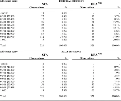
However, as reported above, while DEA attributes any deviation to the frontier to estimated inefficiency component, technical efficiency computed from SFA corresponds to real inefficiency devoid of noise effects. Therefore, distribution of scores on the sample should give us more information about differences between estimated technical efficiencies calculated from SFA and DEA. As reported in Table 12, findings arisen form DEA (under variable returns to scale) suggest that the main share of farms reveals an optimal degree of efficiency (more than 20%), while a full efficiency is achieved by less than 2% of the sample in case of estimation trough SFA model. On the contrary, the share of farms that report an efficiency score close to the frontier (0.900 < TE < 1.000) amounts to 34.9% and 14.9% for SFA and DEA models, respectively. It might depend on the DEA method of constructing the frontier and its inherent difficulty under variable returns to scale hypothesis to detect the real efficiency due to possibility of overestimating number of full efficient units (Førsund, 1992; Kumbhakar and Tsionas, 2008).
variable returns to scale for the DEA frontier, the SFA model holds no real advantage over DEA in estimating technical efficiency scores and efficiency variability.
Table 12 – Frequency distributions of technical and scale efficiency estimates from the SFA and from DEA VRS models
Efficiency score TECHNICAL EFFICIENCY
SFA DEA VRS
Observations % Observations %
< 0.200 13 4.0% - -
0.201 – 0.300 27 8.4% 12 3.7%
0.301 – 0.400 17 5.3% 27 8.5%
0.401 – 0.500 26 8.1% 51 15.9%
0.501 – 0.600 22 6.9% 42 13.1%
0.601 – 0.700 23 7.1% 39 12.1%
0.701 – 0.800 19 5.9% 18 5.6%
0.801 – 0.900 57 17.8% 18 5.6%
0.901 – 0.999 112 34.9% 48 14.9%
1.000 5 1.6% 66 20.6%
Total 321 100.0% 321 100.0%
Efficiency score SCALE EFFICIENCY
SFA DEA VRS
Observations % Observations %
< 0.200 3 0.9% - -
0.201 – 0.300 8 2.5% 3 0.9%
0.301 – 0.400 9 2.8% 9 2.8%
0.401 – 0.500 17 5.4% 6 1.9%
0.501 – 0.600 18 5.6% 9 2.8%
0.601 – 0.700 18 5.6% 6 1.9%
0.701 – 0.800 34 10.6% 24 7.4%
0.801 – 0.900 54 16.8% 57 17.8%
0.901 – 0.999 141 43.9% 147 45.8%
1.000 19 5.9% 60 18.7%
Total 321 100.0% 321 100.0%
Concerning scale efficiency estimates, there are significant differences from the two methods (for α = 0.05). The mean scale efficiency relative to SFA model (0.818) is lower than that estimated from the DEA model (0.894). Table 12 shows that distribution of scale efficiency scores on the sample is similar between DEA and SFA measures, except to share of farms that reveal full efficiency. Using SFA model, 5.9% of the sample reports an optimal degree of scale efficiency, while this percentage amounts to 18.7% in case of application of DEA model. According to Førsund (1992), it could depend on identification problem of full efficient observations by part of DEA model because units located at the end of size distribution may be identified as efficient simply for lack of other comparable units. Vice versa, since the mean DEA scale efficiency score is higher than the correspondent SFA measure, a larger number of full efficient farms computed trough DEA might be attributed to real differences due to the empirical methodologies adopted to estimate the frontier and efficiency.
methodological approach might influence estimation of scale efficiency. This is a relevant point arisen from this study and it confirms how scale efficiency (and generally efficiency measures) can vary according to the model adopted for estimating frontier function on a given sample of farms, as underlined or found by several authors (Banker
[image:22.595.78.517.207.357.2]et al., 1986; Førsund. 1992; Sharma et al., 1997; Wadud and White, 2000; Ruggiero, 2007).
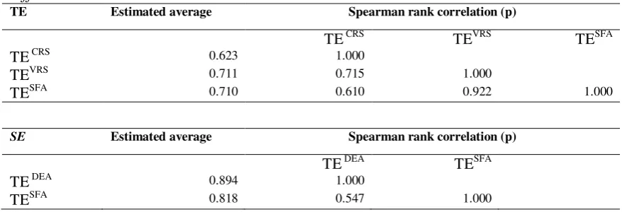
Table 13 – Spearman rank correlation matrix of TE and SE rankings obtained from different models
TE Estimated average Spearman rank correlation (p)
TE CRS TEVRS TESFA
TE CRS 0.623 1.000
TEVRS 0.711 0.715 1.000
TESFA 0.710 0.610 0.922 1.000
SE Estimated average Spearman rank correlation (p)
TE DEA TESFA
TE DEA 0.894 1.000
TESFA 0.818 0.547 1.000
However, scale efficiency is found to be high, on average, from application of both methods. Since the technical efficiency score is, on average, lower than the scale efficiency score this implies that the greater portion of overall inefficiency in the sample might depend on producing below the production frontier than on operating under an inefficient scale. It means that the search for an optimal scale would not become a priority for citrus farmers, while it would be a priority increasing ability in using disposable technical inputs because of technical efficiency is higher than scale efficiency. In other terms, it means that farm size issue is much less important relative to the amount of technical efficiency
Furthermore, both DEA and SFA analyses suggest that scale inefficiency is mainly due to the farms operating under a sub-optimal scale. Indeed, we found that the most of the observed farms operate under increasing returns to scale for both methods also if the incidence of sub-optimal scale farms on the total citrus farms is higher if scale efficiency is measured trough SFA (66.3% vs. 79.4% for DEA and SFA, respectively). In addition, both analyses suggest that these sub-optimal-scale farms must have adjusted their output levels to a greater extent than the supra-optimal-scale ones. In these latter farms, the margin that separate them from the optimal scale seem to be really narrow, as suggested by the estimated scale efficiency that is, on average, close to unity (SE equal to 0.934 and 0.978 for DEA and SFA, respectively), while in the sub-optimal scale farms this margin is large (scale efficiency equal to 0.692 and 0.775 for DEA and SFA, respectively). Therefore it implies that scale inefficiency is mainly due to the farms operating under a suboptimal scale.
(e.g., vast land fragmentation, huge number of single-household farms, insignificant presence of land market). They usually do not have adequate farming implements or up-to-date technologies or they are not allowed to reach their optimum size under their particular circumstances. Thiele and Brodersen (1999) argue that these market and structural constraints are among the main factors that usually impede achievement of efficient scales by part of farmers. Regarding the Italian citrus farms, Idda (2006) and Carillo et al. (2008) found that, often, the input mix is unbalanced (with respect to the rational and efficient composition of the input bundle) in favour of a high ratio of capital to land area and labour to land area. This should be mainly caused by a scarce flexibility in the land market, which forces farmers to expand the use of other inputs (except for land), especially labour and capital, with practical implications on the scale efficiency. Therefore, the presence of a quasi-fixed factor such as land should negatively affect scale efficiency and should favour exhibition of increasing returns to scale.
Estimation of the (technical and scale) inefficiency effects show that it is slightly sensitive to the method used. Computation of DEA reveals that technical efficiency should significant depend on farm size (positive effect), on number of plots of land and (negative effect) and on location in a less-favoured area (negative effect). Application of SFA approach seem to confirm these findings because the only three factors appeared significant by a statistical point of view are those mentioned above and the sign of the effect is the same estimated from DEA.
It must be underlined that the fact that farm size affect technical efficiency is an empirical finding that is often found in the literature, even if studies show controversial results about the relationship between technical efficiency and farm size (Sen 1962; Kalaitzandonakes et al. 1992; Ahmad and Bravo-Ureta 1995; Alvarez and Arias 2004). On the other hand, estimation of scale efficiency effects show similar results in DEA and SFA application. In both analysis farm size (positive effect), number of plots of land (negative effect) and geographical location of farm should be the main factors that affect scale efficiency in the Italian citrus farming.
6.CONCLUSIONS
This paper aimed to evaluate technical and scale efficiencies on a sample of citrus farms located in Italy. Using two different approach (parametric and non parametric) we found that some margins exist to increase efficiency, both using better disposable inputs and operating on a more appropriate scale. Empirical findings arisen from the two methods used suggest that the overall inefficiency should depend on producing below the production frontier and on operating under a rational scale.
The former reason might be more important since technical inefficiency appears greater than scale inefficiency.
However, the estimated technical efficiency from the SFA model is substantially at the same level of this estimated from DEA model, while the scale efficiency arisen from SFA is larger than this obtained from DEA analysis.
Finally, the correlation between the efficiency rankings of the two approaches is positive and significant both for technical and scale efficiency ranking, also if magnitude of the Spearman rank correlation coefficient is higher for technical efficiency than for scale efficiency rankings.
REFERENCES
Ahmad M, Bravo-Ureta B (1995) An econometric analysis of dairy output growth. American
Journal of Agricultural Economics 77: 914-921.
Aigner DJ, Lovell CAK, Schmidt, PJ (1977) Formulation and Estimation of Stochastic Frontier Production Function Models. Journal of Econometrics 6: 21-37.
Alvarez A, Arias C (2004) Technical Efficiency and Farm Size: A Conditional Analysis.
Agricultural Economics 30: 241-250.
Atkinson SE, Cornwell C (1994) Estimation of Output and Input Technical Efficiency Using a Flexible Functional Form and Panel Data. International Economic Review 35: 245-255. Balk BM (2001) Scale Efficiency and Productivity Change. Journal of Productivity Analysis 15:
159-183.
Banker RD (1984) Estimating the Most Productive Scale Size using Data Envelopment Analysis. European Journal of Operational Research 17: 35-44
Banker RD, Charnes A, Cooper WW (1984) Some Models for Estimating Technical and Scale Inefficiency in Data Envelopment Analysis. Management Science 30: 1078-1092.
Banker RD., Conrad RF, Strauss RP (1986) A Comparative Application of Data Envelopment Analysis and Translog Methods: An Illustrative Study of Hospital Production. Management
Science 32: 30-44.
Battese GE, Coelli TJ. (1995) A Model for Technical Inefficiency Effects in a Stochastic Frontier Production Function for Panel Data. Empirical Economics 20: 325-232.
Battese GE, Corra GS (1977) Estimation of a Production Frontier Model: With a Generalized Frontier Production Function and Panel Data. Australian Journal of Agricultural Economics 21: 169-179.
Bjurek H, Hjalmarsson L, Forsund FR (1990) Deterministic Parametric and Non parametric Estimation of Efficiency in Service Production. A Comparison. Journal of Econometrics 46: 213-227.
Bohrnstedt GW, Knoke D (1994) Statistics for Social Data Analysis. F.E. Peacock Publishers Inc., Itasca.
Bravo-Ureta BE, Solis D, Moreira Lopez V, Maripani JF, Thiam A, Rivas T (2007) Technical Efficiency in farming: a Meta-Regression Analysis. Journal of Productivity Analysis 27: 57-72.
Carillo F, Doria P, Madau FA (2008) L’analisi della redditività delle colture agrumicole attraverso l’utilizzo dei dati RICA. Stilgrafica, Rome.
Charnes A, Cooper WW, Seiford LM (1994) Data Envelopment Analysis: Theory, Methodology
and Application. Kluwer Academics, Dordrecht, Boston and London.
Charnes A, Cooper WW, Rhodes E (1978) Measuring the Efficiency of Decision Making Units.