Probabilistic analysis of QoS aware service composition with Explicit Environment Models

BIROn - Birkbeck Institutional Research Online

Zhou, Y. and Han, Tingting and Chen, Taolue and Zhou, S. (2019)

Probabilistic analysis of QoS-aware service composition with Explicit

Environment Models. IET Software , ISSN 1751-8806. (In Press)

Downloaded from:

Usage Guidelines:

Please refer to usage guidelines at

or alternatively

Probabilistic Analysis of QoS-Aware Service Composition with

Explicit Environment Models

Yu Zhou, Tingting Han, Taolue Chen, Shiqi Zhou

November 6, 2019

Abstract

Service composition is one of the primary ways to provide value-added services on the Internet. Quality-of-Service (QoS) represents a crucial indicator for the underlying composition policy adoption, but it is highly influenced by various environmental factors. Existing composition strategies rarely take the influence of environment into consideration explicitly, which may lead to sub-optimal composition policies in a dynamic environment. In this paper, a model-based service composition approach is proposed. Given the user request, it is possible to first find a set of matching abstract web services (AWSs), and then pull relevant concrete web services (CWSs) based on the AWSs. The set of CWSs can be modelled as a Markov decision process (MDP). In addition, we model the environment as a fully probabilistic system, capturing changes of environment probabilistically. The environment model can be further composed with the MDP from the service models, obtaining a monolithic MDP. The policy of which corresponds the selection of concrete services. We demonstrate how probabilistic ver-ification techniques can be used to find the optimal service selection strategy against their QoS and the environment change. A distinguished feature of our approach is that the QoS of services, as well as the dynamic of environment change, are made parametric, so that the formal analysis is adaptive to the environment which is of paramount importance for autonomous and self-adaptive systems. Examples and experiments confirm the feasibility of our approach.

KEYWORDS

Service Composition, Markov Decision Process,

Para-metric Model Checking, Quality-of-Service

1

Introduction

Web service has nowadays become one of the most pop-ular forms of software function provision on the Internet. Despite an increasing number of individual services, more complex and systematic user tasks pose a high demand for the composition of underlying atomic services. Web ser-vice composition has been an active research topic dur-ing the last decade from both the theoretical and practical points of view [1, 2, 3, 4, 5]. During composition, Quality-of-Service (QoS) usually emerges as the primary concern, since it is often the case that multiple services provide sim-ilar or the same functionality, but with significantly differ-ent QoS measures. Supporting QoS-aware service compo-sition is a challenging task due to the inherent uncertainty from the environment [6, 7, 8]. For instance, it is con-ceivable that services may exhibit fluctuating performance ensuing the vibrating network bandwidth. A majority of existing approaches, however, merely model the QoS with pre-defined values (which are acquired by, e.g., historical data or experiments), and reduce the composition prob-lem to an optimisation probprob-lem, such as [9, 10]. These approaches, while being simple, disregard the uncertain-ties from the environment which may have a significant impact on QoS in real settings.

tim-ing, security issues, network performance and any other factors that might affect the QoS. A mode is a typical con-figuration of an environment. For instance, the mode can be “rainy and peak times” and switch to “cloudy and off-peak times" or the security level is “severe” and switch to “medium", etc. (2) Parameter uncertainty. QoS of individ-ual web services, or the probabilities of the environment modes switch are numeric values. They are acquired via monitoring, test, experiments, etc, and are essentially of statistical nature. It is virtually impossible to obtain a pre-cise value for them. For instance, the time to arrive at an airport at peak hours is one hour on average, but can be in the range of, for instance, 0.8 to 2 hours. To have a more accurate analysis of the time, it is suggested to use a parameter (variable) to represent some probability (e.g., the probability to turn from sunny to cloudy) or measure (e.g., the time it takes to get somewhere), and to explore how the property of interest depends on the concrete pa-rameter values.

To address these issues, in this paper, we propose a parametric Markov decision process based approach to support the analysis of QoS-aware service composition. Apart from modelling web services and their composi-tion, we also explicitly model the mode switch of envi-ronments using a probabilistic model. The probabilities can usually be extracted from the real-time weather focast, live traffic data, on-going network performance re-ports, or other domain-specific historical data that might be related and informative. The parameters may appear as the transition probabilities in the environment model, or as the QoS measures in the service models. Consider the following scenario. A customer wants to buy a product online. The person should make a decision in (1) which shopping websites, e.g., Amazon or Ebay; (2) which shop, e.g., Amazon or third party shops; (3) delivery services at different speeds and rates, e.g., expedite but expensive same-day delivery or free 3-5 days delivery; and (4) pay-ment methods, including credit card fees, possible dis-counts and cashbacks, etc. In this example, depending on the customer’s priorities and needs, different decisions could been made. For instance, if the customer makes this purchase for a birthday party that evening, then only shops that provide same-day delivery would be chosen. If the product is not urgently needed, then the most economical way of delivery would be used.

Our system takes in the user requirements, finds the

ab-stract web services (the type-matching services that are used in the workflow at a high level), searches the eligible and compatible concrete web services (the services that are really used) and builds models for both the web ser-vices and the environment. Depending on the user’s ob-jectives and constraints, the system recommends the best strategies or decisions in choosing concrete web services. The system can then invoke and compose the chosen web services and deliver the final result to the user.

During the process of composition, we observe that al-though services are standalone entities, at times, a client’s requirements would greatly reduce the number of poten-tially usable web services. For instance, if a traveller would like to bring a pet along, this basically excludes the option of taking the airplane. Or if a traveller needs to use a lift to get to the platform of an underground train, but the closest station does not provide a lift facility, the underground option could be taken off the table. In our approach, by formalising the user’s requirements, we can reduce the state space at an early stage instead of enumer-ating all the composition possibilities.

Contribution The main contributions of the paper are

summarised as follows:

• A modelling language including both the web vice model and the environment model; the web ser-vice model is extended with variables and pre-/post-conditions to facilitate modelling of composition. The approach, which follows the “separation of concerns" rationale, provides the maximum modularity and flexi-bility with regards to web services and environments. In other words, we separate the modelling of web services and environment so that either can easily be replaced by other matching services or environment.

• Automated analysis with fully-fledged tool support. Our analysis is parametric, and accounts for Pareto op-timality, which is indispensable when factoring in a dynamic environment. More technically, our analysis benefits from advanced, automated probabilistic veri-fication tools, and supports analysis of objectives akin to QoS-aware service composition (based on expected reachability rewards rather than discounted sum which is a least worst surrogate).

Structure of the paper.The rest of the paper is structured

3 gives background information and preliminaries. We de-tail our approach in Section 4, and conclude our paper in Section 5.

2

Related Work

In this section, we briefly overview some most relevant work with focus on QoS-aware service composition.

Canfora et al. [11] proposed a genetic algorithm based approach for QoS service composition. Particularly, ge-netic algorithms are leveraged to determine a set of con-crete services to be bound to abstract services. The ap-proach only supports single objective (fitness) function, not the parametric analysis. Zhou et al. [12] proposed a model based approach to assure the behaviour consis-tency of service composition during runtime evolution. Wang et al. [13] studied the incomplete information prob-lem of selecting one service among a set of candidates, and employed dynamic pricing strategy to compose web services with the maximum utility and the lowest costs. Ren et al. [14] modelled the service composition prob-lem as a Markov decision process to satisfy the require-ments of both functional aspects and non-functional ones, and then a Q-learning based algorithm is applied to solve the model. Rodriguez-Mier et al. [15] proposed a hybrid approach for service composition which could produce a composition strategy that minimizes a single objective QoS function. These pieces of work mainly cast the ser-vice composition into a constraint solving problem and leverage optimisation techniques to provide optimal solu-tions. More remotely, genetic algorithms and swarm op-timisation algorithms, have also been used in self-adapted systems [16, 17].

Apart from using different techniques, our work is grounded on a formal framework with rigorous lan-guages for modelling and specification, as well as well-established tool support. One of the advantages of our ap-proaches lies in the theoretical guarantee it provides, ow-ing to the underlyow-ing probabilistic verification. Computa-tionally, our approach essentially utilises specific numeri-cal methods for solving Markov decision processes (e.g., value iteration) so could be more efficient than the gen-eral optimisation methods, especially when their objective functions are overly complicated.

Wang et al. [9, 10] proposed approaches based on

re-inforcement learning to enable adaptive and dynamic ser-vice composition. During composition, the multi-agent reinforcement learning technique is employed to select the concrete service. Jungmann et al. [18] studied the prob-lem of functional discrepancy during service composition and presented an automated approach for adaptive ser-vice composition. Moustafa et al. [19] proposed a rein-forcement learning based approach to support QoS-aware service composition with conflicting objectives. Similar to our work, they use Markov decision process to model the service composition. However, they neither explicitly model the environment factors, nor support the parame-terisation. On a more technical level, these authors usu-ally take discounted sum of rewards as the optimisation objective in MDPs, which is a tradition in the reinforce-ment learning literature, but which arguably is not suitable for service composition purposes. Bashari et al. [20] pro-posed an automated approach to reconfigure the service composition strategy from the changing environment, the reconfiguration policies were derived from software prod-uct line techniques. Zhang et al. [8] recognised the neces-sity of an explicit environment model during service se-lection and proposed a QoS-aware monitoring approach. However, this approach is restricted to QoS monitoring purposes instead of service composition.

There are several service composition patterns, for in-stance, atomic pattern, sequential patten, multiplication pattern, parallel pattern and combined pattern, etc [21]. Our work focuses on sequential patterns. Moreover, be-cause of the similarity of web service composition and business process modelling [22], our methods can be ap-plied to the analysis and optimisation of business pro-cesses, which would complement the existing approaches [23, 24, 25].

personalised QoS values. [29] proposed a learning based approach for QoS value prediction which integrate multi-dimensional context. Particularly, the approach adopts an unsupervised encoder-decoder framework to generate a hidden feature based on which the similarity between two context entities could be calculated more accurately. In [30], a model was proposed which can embed policies to calculate composite service performance, and based on which, the composite service’s performance could be pre-dicted. Different from the work, our approach addresses the QoS awareness in the context of service composi-tion despite the fact that some common composicomposi-tion tech-niques might have been employed in the previous work mentioned above.

3

Preliminaries

In real-world settings, the web services are hosted in a dy-namic and unstable Internet-based environment, which in-evitably makes deterministic models inappropriate. Prob-abilistic model checking has been widely applied in quan-titatively analysing systems which exhibit stochastic fea-tures. Properties could be specified based on the two prob-abilistic temporal logics, i.e., Probprob-abilistic Computation Tree Logic (PCTL) [31] and Continuous Stochastic Logic (CSL) [32].

We leverage the PRISM model checker [33] to construct the probabilistic model. PRISM is a leading open-source model checker and has been successfully applied in many fields, such as communication protocols, distributed algo-rithms and some other systems of specific subjects like bi-ology. PRISM supports a set of probabilistic models, such as Markov decision processes extended with costs and re-wards. Therefore, a wide range of quantitative measures related to model behaviours could be analysed. In addi-tion, PRISM has also integrated the support for a para-metric analysis of these models.

Definition 3.1 (FPS) Afully probabilistic systemis a

tuple(𝑆, 𝑠₀,𝐏), where 𝑆 is a set of states with 𝑠₀ ∈ 𝑆

being the initial state; and𝐏 ∶ 𝑆×𝑆 → [0,1]is the transition probability function such that for all states𝑠∈

𝑆,∑_𝑡∈𝑆𝐏(𝑠, 𝑡) ∈ [0,1].

Definition 3.2 (MDP) AMarkov Decision Processis

a tuple(𝑆, 𝑠₀, 𝐴,𝐏, 𝑅), where

• 𝑆is a set of states with𝑠₀∈𝑆being the initial state;

• 𝐴is a set of actions;

• 𝐏 ∶ 𝑆×𝐴×𝑆 → [0,1]is the transition probability function such that for all states𝑠∈𝑆and actions𝛼 ∈

𝐴,∑_𝑡∈𝑆𝐏(𝑠, 𝛼, 𝑡) ∈ {0,1}; • ∶𝑆→ℝ_≥0.

For each state𝑠∈𝑆and action𝛼, if∑_𝑡∈𝑆𝐏(𝑠, 𝛼, 𝑡) = 1, then we say the action𝛼isenabledin𝑠.

Policies play a crucial role in the analysis of MDPs. For our purposes, it suffices to considersimplepolicies, in which for each state𝑠, the policy fixes one of the

en-abled actions at𝑠and selects the same action every time

when the system resides in𝑠. Thus, the choices made by a

simple policy are independent of history. Formally, a sim-ple policy is a function𝜎∶𝑆→𝐴𝑐𝑡such that𝜎(𝑠)is one of the actions enabled at state𝑠. Apathin MDP under𝜎

is an infinite sequence of states𝜌=𝑠₀𝑠₁⋯such that, for

all𝑖 ≥ 0,𝐏(𝑠_𝑖, 𝛼, 𝑠_𝑖+1) > 0for𝛼 = 𝜎(𝑠_𝑖). Let𝑃 𝑎𝑡ℎ_,𝜎

be the set of paths inunder𝜎. Let𝑃 𝑎𝑡ℎ_,𝜎(𝑠)be the subset of paths that start from𝑠, and𝑃 𝑟_,𝜎be the

stan-dardprobability distributionover𝑃 𝑎𝑡ℎ_,𝜎 as defined in

the literature [34, Ch. 10].

Theexpected cumulative reward, or simplycumulative reward, of reaching a set𝐺 ⊆ 𝑆 of goalstates (called 𝐺-states hereafter) in MDP under𝜎, denoted _,𝜎(𝐺),

is defined as follows: First, let ,𝜎(𝑠, 𝐺) be the

ex-pected value of random variable𝑋∶𝑃 𝑎𝑡ℎ_,𝜎(𝑠)→ℝ_≥0

such that (i) if 𝑠 ∈ 𝐺 then𝑋(𝜌) = 0, (ii) if 𝜌[𝑖] ∉ 𝐺

for all𝑖 ≥0then𝑋(𝜌) = ∞, and (iii) otherwise𝑋(𝜌) =

∑𝑛−1

𝑖=0 𝑅(𝑠𝑖)where𝑠𝑛∈𝐺and𝑠𝑗 ∉𝐺for all𝑗 < 𝑛. Then,

let_,𝜎(𝐺) =,𝜎(𝑠0, 𝐺).

4

Our approaches

4.1

Overview

Figure 1 gives an overview of our approach. A user request specifies the specification of what the user needs (e.g., in-put, outin-put, type of service, etc). When a user sends a request𝑟, the web service configurator matches the

Figure 1: Overview of our approach

the user request. The result is a set𝔸 of AWSs. With

additional constraints specified in the user request, AWSs which do not satisfy the user’s needs are excluded from𝔸.

The result becomes𝔸⇂𝑟.

The next step is to pull the concrete web services (CWSs) corresponding to𝔸⇂𝑟, based on which a Markov

Decision Process (MDP) 𝔸⇂𝑟 will be built. In case

that the environment model is available, it will be

inte-grated resulting the MDP model𝔸⇂𝑟||which respects

the changes in the environment. The formal definitions of AWS, CWS and environment model are given in Sec-tion 4.2.

Recall that there might be environment or parameter un-certainty in either the service models or environment mod-els, and the uncertainties are modelled by parameters. In these cases, we will have a parametric MDP (i.e., either

𝑝𝔸⇂𝑟or𝑝𝔸⇂𝑟||). Parameter analysis can then be

ap-plied to the parametric MDPs against user QoS require-ments. The results may be closed-form functions or plots, which describe the region of the feasible solutions. One can instantiate the parameters as per any point of the re-gion obtaining a (non-parametric) MDP, whereby obtain an acceptable selection/combination of web services.

In case that the MDP is not parametric, probabilistic model checking can be applied on the user QoS

require-ment. Either boolean or numeric values may be returned together with a policy that indicates which concrete web services to select and compose.

4.2

Models and specifications of web service

selection

4.2.1 Web service models

There are different ways by which individual services can be integrated to build a process, e.g., sequential, paral-lel, conditional, iterative, etc. In this paper, we focus ex-clusively on the sequential composition of web services, which is the most fundamental and widely used pattern in service composition. Other ways of composition are con-vertible to the sequential composition [35] under a config-urator, which acts as a policy, resolving all the uncertain-ties in the composition models. Note that the configurator in this paper is a general manager that does web service se-lection, composition and adaptation. We refer the readers to [35] for more details.

and positive/negative pre-/post-conditions. A similar con-cept of AWS can be found in e.g., [36].

Definition 4.1 (Abstract web service, AWS)

An abstract web service is defined as a tuple

 = (𝑂𝑃 , 𝐼 , 𝑂, 𝑝+, 𝑝−, 𝑒+, 𝑒−), where each compo-nent comprises a set of (atomic) propositions.

Here the atomic propositions represent the status and/or properties of a state or condition. Intuitively,𝑂𝑃 is the

semantic description of the service, in the form of a mem-bership statement of a class in an ontology [36]. Input𝐼

and output𝑂represent signature information (basic input

and output data types) of a service. They ensure syntac-tically correct solutions and a successful execution. On the other hand, required pre-conditions𝑝+, prohibited

pre-conditions𝑝−, positive post-conditions 𝑒+, and negative

post-conditions𝑒−represent semantic information which

reduces the set of syntactically correct solutions to only those solutions that are really useful. We reserve two propositions𝑖𝑛𝑖𝑡 and𝑒𝑛𝑑 for 𝑝+ and𝑒−, respectively to

indicate the start and end of the sequential composition of the AWSs as shown in Def. 4.4.

Example 4.2 Suppose Adam would like to go from his

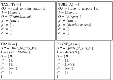
home in city A to another city B. He could choose to go by train or plane, and whether to take taxi or tube to ei-ther the train station or the airport. Suppose ei-there are one train station, two airports that have connection to B. The abstract web services in this case could be TAXI_TS, TAXI_A1, TAXI_A2, TUBE_TS, TUBE_A1, TRAIN (train from A to B) and PLANE_A1, PLANE_A2. More specifi-cally, TAXI_TS and TAXI_A1 mean the taxi service to the train station, and Airport_1, respectively, and PLANE_A1 means the airlines from Airport_1 to city B. Given the input (starting location) and the output (destination), we show some of the AWSs in Fig. 2.

Recall that the keyworsdinitandendmean that the cor-responding AWSs are the initial and last service along the composition. In PLANE_A1, pets are not allowed on the planes and are restricted by 𝑝−. In TUBE_A1, the

dis-able access is not availdis-able at the local station, which is excluded by𝑝−.

To sequentially compose two AWSs 1 and2, one

needs to ensure that1and2arecompatible, which

en-tails the following three conditions: (a) the input of2is

TAXI_TS = {

𝑂𝑃= {taxi_to_train_station}, 𝐼= {ℎ𝑜𝑚𝑒},

𝑂= {𝑇 𝑟𝑎𝑖𝑛𝑆𝑡𝑎𝑡𝑖𝑜𝑛}, 𝑝+_{= {𝑖𝑛𝑖𝑡},}

𝑝−_{= {},}

𝑒+_{= {},}

𝑒−_{= {}}

}

TUBE_A1 = {

𝑂𝑃= {tube_to_airport_1}, 𝐼= {ℎ𝑜𝑚𝑒},

𝑂= {𝐴𝑖𝑟𝑝𝑜𝑟𝑡1}, 𝑝+_{= {𝑖𝑛𝑖𝑡},}

𝑝−_{= {𝑑𝑖𝑠𝑎𝑏𝑙𝑒 𝑎𝑐𝑐𝑒𝑠𝑠},}

𝑒+_{= {},}

𝑒−_{= {}}

} TRAIN = {

𝑂𝑃= {train_to_city_B},

𝐼= {𝑇 𝑟𝑎𝑖𝑛𝑆𝑡𝑎𝑡𝑖𝑜𝑛},

𝑂= {𝐵},

𝑝+_{= {},}

𝑝−_{= {},}

𝑒+_{= {𝑒𝑛𝑑},}

𝑒−_{= {}}

}

PLANE_A1 = {

𝑂𝑃= {plane_to_city_B},

𝐼= {𝐴𝑖𝑟𝑝𝑜𝑟𝑡1},

𝑂= {𝐵},

𝑝+_{= {},}

𝑝−_{= {𝑝𝑒𝑡𝑠},}

𝑒+_{= {𝑒𝑛𝑑},}

𝑒−_{= {}}

}

Figure 2: Example AWSs

a subset of the output of1; this is to guarantee that all

the inputs of the second AWS would be available as a re-sult of the outputs from the first AWS. (b) the required pre-condition of 2 should be a subset of the positive

post-condition of1; (c) the intersection of the

prohib-ited pre-condition of2 and the positive post-condition

of1should be empty. Formally,

Definition 4.3 Two AWSs _1 =

(𝑂𝑃₁, 𝐼₁, 𝑂₁, 𝑝+

1, 𝑝 − 1, 𝑒

+ 1, 𝑒

−

1) and 2 = (𝑂𝑃2, 𝐼2, 𝑂2,

𝑝+

2, 𝑝 − 2, 𝑒

+ 2, 𝑒

−

2)arecompatible, written1⋈2, if

(𝑎) 𝐼₂⊆ 𝑂₁; (𝑏) 𝑝+

2 ⊆ 𝑒

+

1; (𝑐) 𝑝 −

2 ∩𝑒

+ 1 = ∅.

As expected, when two AWSs are compatible, one can define their sequential composition, yielding another AWS.

Definition 4.4 (Service composition) Given two AWSs

1 = (𝑂𝑃1, 𝐼1, 𝑂1, 𝑝+1, 𝑝 − 1, 𝑒

+ 1, 𝑒

−

1) and 2 =

(𝑂𝑃₂, 𝐼₂, 𝑂₂, 𝑝+₂, 𝑝−₂, 𝑒+₂, 𝑒−₂)such that 1 ⋈ 2. The sequential composition 1⊗2 of1 and 2 is de-fined as 1 ⊗ 2 = (𝑂𝑃 , 𝐼 , 𝑂, 𝑝+, 𝑝−, 𝑒+, 𝑒−) where

𝑂𝑃 = 𝑂𝑃1∪𝑂𝑃2,𝐼 =𝐼1,𝑂 = 𝑂2,𝑝+ = 𝑝+₁ ∪𝑝+₂,

𝑝−=𝑝−

1 ∪𝑝

− 2,𝑒

+_=𝑒+

1 ∪𝑒

+ 2,𝑒

−_=𝑒−

1 ∪𝑒

− 2.

same type lies in the quality of services. To this end, a concrete WS is defined as follows.

Definition 4.5 ((Concrete) web service, CWS)

A (concrete) web service is defined as a tuple

 = (ID,AWS,QoS), where ID is the identifier of the web service; AWS is the abstract web service (service type); QoS is the quality of the service represented by an (𝑛 + 1)-tuple ⟨𝑄₀, 𝑄₁,⋯, 𝑄_𝑛⟩, where each 𝑄_𝑖, 𝑖∈ {0, ..., 𝑛}denotes a QoS attribute of the CWS.

We reserve𝑄₀as a primary QoS, representing the

avail-ability of the service, usually given as the probavail-ability of the service being successfully invoked.

Example 4.6 _1 = (MiniCab, TAXI_TS,

⟨𝑄₀, 𝑄_𝑡, 𝑄_𝑠, 𝑄_𝑐⟩) is a taxi service called MiniCab.

𝑄₀ = 0.95is the probability that a minicab is available and arrives on time; 𝑄_𝑡 = 0.9ℎ shows how fast the

service is;𝑄_𝑠 = 0stopsshows that it is a direct journey and no transfer is required;𝑄_𝑐=£50shows how much it charges.

2 = (Uper1,TAXI_TS,⟨𝑄0 = 0.9, 𝑄𝑡 = 0.9ℎ, 𝑄𝑠 =

0, 𝑄_𝑐 = £40⟩)is another taxi service called Uper, which is cheaper than MiniCab, but with less availability.

3 = (Line1&2, TUBE_A1, ⟨𝑄0 = 0.99, 𝑄𝑡 =

1ℎ, 𝑄_𝑠 = 1, 𝑄_𝑐 = £5⟩)is a tube service. Note that the probability of a tube running on time (0.99) is much higher than that of a taxi. But this service requires one transfer during the journey.

4 = (Express,TRAIN,⟨𝑄0 = 0.98, 𝑄𝑡 = 2ℎ, 𝑄𝑠 =

0, 𝑄_𝑐=£100⟩)is an express train and it provides fast and direct connections, but is rather expensive.

5 = (Local, TRAIN,⟨𝑄0 = 0.90, 𝑄𝑡 = 5ℎ, 𝑄𝑠 =

2, 𝑄_𝑐 =£50⟩)is connected by several local trains, which is relatively slow and needs 2 transfers, but is economical.

After deploying the abstract web service composition at a higher level, the web service configurator then picks a CWS for each AWS so that the concrete chain of services satisfies its own need subject to certain constraints. In-spired by [18] which used transition systems to model the composition, we construct an MDP to model the sequen-tial composition of CWSs. Given a set of candidate CWSs

ℂ, we can generate an MDP as follows.

1_{A fictitious company}

Definition 4.7 (MDP for composition) Given a setℂof

candidate CWSs, the MDP is

ℂ= (𝑆, 𝑠0, 𝐴,𝐏,, 𝐴𝑃 , 𝐿), where

• 𝑆 ⊆ℂ∪ {𝑠₀,End}, with𝑠₀the initial state and End a

special state indicating the end of a process; • 𝐴𝑃is the set of atomic propositions;

• 𝐿∶𝑆→2𝐴𝑃_{is a labelling function that assigns subset}

of𝐴𝑃 to each state;

• The set of actions is𝐴 = {𝛼 ∣𝛼 = .ID, ∀ ∈ ℂ} ∪ {fin};

• The transition probabilities are defined as - 𝐏(𝑠₀, 𝛼,𝑗) =𝑞and𝐏(𝑠₀, 𝛼,𝑗) = 1 −𝑞, if

⋆ 𝑗 ∈ℂ,

⋆ 𝑖𝑛𝑖𝑡 ∈ 𝑗.𝑝+(𝑗 is one of the starting web

ser-vices),

⋆ 𝛼 = 𝑗.ID (action is the ID of the starting web

service), and

⋆ 𝑞=𝑗.𝑄₀(probability of successfully calling

ser-vice𝑗);

- 𝐏(𝑖, 𝛼,𝑗) =𝑞and𝐏(𝑖, 𝛼,𝑗) = 1 −𝑞, if ⋆ 𝑖,𝑗 ∈ℂ,𝛼=𝑗.ID and𝑞=𝑗.𝑄₀, ⋆ 𝑖 ⋈𝑗 (𝑖and𝑗 are compatible);

- 𝐏(𝑗,fin,End) = 1, if𝑗 ∈ℂ,𝑒𝑛𝑑 ∈𝑗.𝑒+.

•  ∶ 𝑆×𝐴×𝑆 → ℝ𝑚 _{is the reward function that}

describes a vector of𝑚(transition) rewards, and for

,′_{∈ℂand𝛼∈𝐴,}

𝑖(, 𝛼,′) =′.𝑄𝑖, if ≠ ′and𝑖(, 𝛼,) = 0

The state space𝑆consists of the set of CWSs and two

extra states - the initial state and the end state. The set of atomic propositions𝐴𝑃 is the set of all atomic

proposi-tions from the AWSs. The set of acproposi-tions𝐴is the ID of

each CWS inℂwith an additional onefin.

To lay out the transition probabilities, we distinguish three cases. (1) Starting from the initial state𝑠₀. A

transi-tion𝑖𝑛𝑖𝑡→𝛼 𝑗can take place if the target state𝑗(which is

ID of the CWS𝑗, and the probability of the transition

is the initial probability of𝑗. (2) For all the

intermedi-ate transitions𝑖 →𝛼 𝑗, we require that the source and

target states (CWSs) are compatible. The actions are the IDs of the target states and the transition probability is the probability successfully calling the target CWS𝑗. This

probability is𝑗.𝑄₀. (3) For the final transition𝑗 →fin End,

we introduce another actionfinand the extra stateEndand the probability is 1.

4.2.2 User requirement

A user requirement defines what a user wants, which guides the configurator to select appropriate abstract or concrete web services. With the user requirement, it is possible to greatly narrow down the range of feasible web services and web service composition, facilitating the se-lection of web services.

We use the same formalism of (abstract) web services for specifying a user requirement so they can be cast into the same framework in a uniform manner. In general, user requirements consist of two parts, the functional require-ment which usually specifies the pre- and post-conditions, but from the user’s perspective; and the non-functional re-quirement which usually focuses on the QoS set by the user. The non-functional requirement is defined as fol-lows.

Definition 4.8 (QoS requirement) Given a QoS

mea-sure𝑄, a QoS requirement is

(i)hard, if it is of the form𝑄∼𝑣where∼ ∈ {<, >,≤,≥} and𝑣is a real number; or

(ii)soft, if it is of the formmax𝑄ormin𝑄, which is to

maximise or minimise Q.

Intuitively, the hard requirements are of the boolean type and should be met, and the soft requirements are of the optimisaton type and the target to be achieved.

Definition 4.9 (User requirement) A user

requirement 𝑟 is defined as a tuple

(𝑜𝑝, 𝑖, 𝑜, 𝑝𝑟𝑒+, 𝑝𝑟𝑒−, 𝑝𝑜𝑠𝑡+, 𝑝𝑜𝑠𝑡−, 𝑟𝑒𝑞), with 𝑜𝑝

de-notes the type of operation the user asks,𝑖and𝑜denoting

input and output, respectively; 𝑝𝑟𝑒+, 𝑝𝑟𝑒− and 𝑝𝑜𝑠𝑡+, 𝑝𝑜𝑠𝑡−are positive and negative pre- and post-conditions; 𝑟𝑒𝑞is a set of QoS requirements.

Example 4.10 A request from a disabled passenger who

would like to bring a pet from home to city B would be

𝑟=(𝑡𝑟𝑎𝑣𝑒𝑙, ℎ𝑜𝑚𝑒, 𝑐𝑖𝑡𝑦𝐵, 𝑝𝑟𝑒+= {𝑑𝑖𝑠𝑎𝑏𝑙𝑒𝑑, 𝑝𝑒𝑡𝑠},

∅,∅,∅,{min𝑄_𝑠, 𝑄_𝑐≤£110}).

Here, min𝑄_𝑠 is to minimise the number of transfers

and 𝑄_𝑐 ≤ £110means the total sum of fare should be no greater than £110.

4.2.3 Web service selection at the abstract level

Given the user requirement, the main task is to select which web services to compose to fulfill the requirement. The selection is carried out at two levels.

At the abstract level, the pre- and post-conditions in the request are crucial to reduce the state space of the MDP for composition. For instance, the positive pre-condition of disabled would rule out the option of taking a tube from a station that does not have disable access; meanwhile, tak-ing a pet would exclude travelltak-ing by plane. The above two restrictions leave the option of taking a taxi connected by a train.

At the concrete level, the composition may only choose the available concreteweb services from the remaining AWSs and build an MDP accordingly. The QoS require-ment can restrict certain policies and CWSs in the MDP, as such policies may induce a model that dissatisfies the QoS requirement.

In the following, we will show how to exclude some AWS from the given set of AWSs and a user request at the abstract level.

Definition 4.11 (AWS exclusion) Given a set of AWSs

𝔸, the corresponding CWSs ℂand a user request 𝑟 = (𝑜𝑝, 𝑖, 𝑜, 𝑝𝑟𝑒+, 𝑝𝑟𝑒−, 𝑝𝑜𝑠𝑡+, 𝑝𝑜𝑠𝑡−, 𝑟𝑒𝑞), we define the set of AWSs exluded by𝑟 as𝔸⇂𝑟 = {𝔸⧵}, for each = (𝑂𝑃 , 𝐼 , 𝑂, 𝑝+, 𝑝−, 𝑒+, 𝑒−) ∈ 𝔸if one of the following is

true

(1)𝑝𝑟𝑒+∩𝑝−_≠∅, (2)𝑝𝑜𝑠𝑡+∩𝑒−_≠∅,

(3)𝑝𝑟𝑒−∩𝑝+≠∅, 𝑜𝑟 (4)𝑝𝑜𝑠𝑡−∩𝑒+≠∅.

ℂ⇂𝑟is the set of concrete web services that belong to𝔸⇂𝑟.

Example 4.12 (Continued from Example 4.10)

{TAXI_TS,TAXI_A1, TAXI_A2,TRAIN,TUBE_TS,

TUBE_A1,PLANE_A1,PLANE_A2} is reduced to

be 𝔸⇂𝑟 = {TRAIN, TAXI_TS} by the user request

𝑟. The corresponding set of concrete web services is ℂ⇂𝑟= {Express,Local,MiniCab,Uper}.

Given a set of AWSs𝔸, the corresponding CWSsℂand

a user requirement𝑟, the resulting MDP is_{ℂ⇂𝑟}.

Intu-itively, the MDP produces all the functionally feasible so-lutions that conform to the user requirement. Each path that starts from 𝑠₀ and ends atEnd represents a way to

compose web services to achieve the functional require-ment of the user.

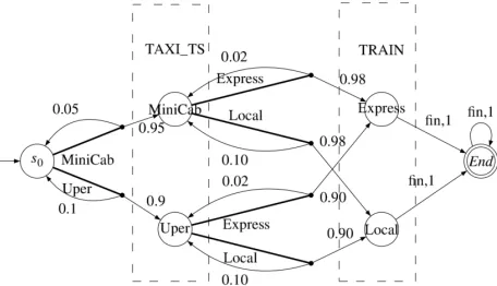
Figure 3: Example of MDP from composing CWSs

Example 4.13 (Continued from Example 4.12) The

MDP for composing set of CWSs ℂ⇂𝑟 is shown as in

Fig. 3, where the probabilities were taken from all the availability probabilities𝑄₀s in Example 4.6.

The exclusion at the AWS level could have led to a (sig-nificant) state space reduction. The MDP in Fig. 3 has 6 states and this is after the exclusion due to positive and negative pre- and post-conditions. The MDP before the exclusion has 18 states, assuming there are 2 CWSs per AWS. In PRISM, due to some auxiliary variables that are used to synchronise, there would be more states than 6 or 18.

Table 1 summarises the number of states and transi-tions before and after the exclusion due to pre- and post-conditions for the travel example. Note that #A is the num-ber of AWSs and #C is the numnum-ber of CWSs per AWS. To

test the magnitude of state space reduction, we scaled the MDP model by enlarging the number of AWSs and CWSs. From the table, the number of states/transitions after the exclusion using p/post-conditions is approximately re-duced by 80% of that before the exclusion.

4.2.4 Web service selection at the concrete level

At the concrete level, the goal is to decide which CWS to select from each type of AWS to satisfy the QoS require-ments. In the MDP, it is to find a policy under which the rewards along the set of paths that go from𝑠₀to theEnd

state fulfiling the QoS requirements.

Remark that there are two types of QoS requirements, the hard ones (e.g.,𝑄_𝑐 ≤ £110,𝑄_𝑡 ≤ 5ℎ) and the soft

ones (e.g.,min𝑄_𝑠minimise the number of transfers). As a

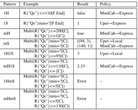
result, we may have eight different patterns of the QoS re-quirements in the first column of Table 2. We write 1H1S a short form of “one hard and one soft requirement” and mHmS is short for “multiple hard and multiple soft re-quirements”, etc.

Six out of the eight QoS patterns can be calculated in PRISM. The only limitation is that there cannot be mul-tiple software requirementandone or more hard require-ments. As a very useful by-product, PRISM provides a policy on how the result is or could be obtained. In other words, the resulting policy points out which concrete web services are being selected.

Example 4.14 • [1H]R{"Qc"}<=110 [F End] is false. The formula asks whether under ALL policies, one can reach city B with no more than £110. The result is false, and a counterexample policy is given - taking MiniCab (£50) + Express train (£100) will add up to £150, which exceeds £110.

• [1S]R{"Qs"}min=? [F End] is 1. The minimum num-ber of transfers is achieved when taking Uper followed by the Express train. The result 1 comes from changing means of transportations.

• [mH] Multi(R{"Qc"}<=200[C], R{"Qs"}<=1[C]) asks whether there exists a policy under which both boolean requirements are true. An evidence policy is provided - taking MiniCab then Express trains. • [mS]Multi(R{"Qc"}min=?[C], R{"Qs"}min=?[C]) is

#A #C _#statesbefore_{#trans #states}after _#trans #A #C _#statesbefore_{#trans #states}after _#trans

8

2 62 91 14 19 11

2 142 191 30 39 4 202 301 42 61 4 842 1181 170 237 6 422 631 86 127 6 2582 3691 518 739 8 722 1081 146 217 8 5842 8441 1170 1689 10 1102 1651 222 331 10 11102 16151 2222 3231 20 4202 6301 842 1261 20 8.4 × 104 _{1.2 × 10}5 _{1.7 × 10}4 _{2.5 × 10}4

30 9302 13951 1862 2791 30 2.8 × 105 _{4.1 × 10}5 _{5.6 × 10}4 _{8.3 × 10}4

#A #C _#statesbefore_{#trans #states}after _#trans #A #C _#statesbefore_{#trans #states}after _#trans

14

2 302 391 62 79 17

2 622 791 126 159 4 3402 4701 682 941 4 13642 18781 2730 3757 6 15542 22051 3110 4411 6 93302 132211 18662 26443 8 4.7 × 104 _{6.7 × 10}4 _{9.4 × 10}3 _{1.3 × 10}4 _{8 3.7 × 10}5 _{5.4 × 10}5 _{7.5 × 10}4 _{1.1 × 10}5

10 1.1 × 105 _{1.6 × 10}5 _{2.2 × 10}4 _{3.2 × 10}4 _{10 1.1 × 10}6 _{1.6 × 10}6 _{2.2 × 10}5 _{3.2 × 10}5

20 1.7 × 106 _{2.5 × 10}6 _{3.4 × 10}5 _{5.0 × 10}5 _{20 3.4 × 10}7 _{5.0 × 10}7 _{6.7 × 10}6 _{1.0 × 10}7

30 8.4 × 106 _{1.2 × 10}7 _{1.7 × 10}6 _{2.5 × 10}6 _{30 2.5 × 10}8 _{3.7 × 10}8 _{5.0 × 10}7 _{7.5 × 10}7 Table 1: Comparison of #states and #transitions before/after AWS exclusion

Pattern Example Result Policy

1H R{"Qc"}<=110[F End] false MiniCab→Express

1S R{"Qs"}min=?[F End] 1 Uper→Express

mH Multi(R{"Qc"}<=200[C], true MiniCab→Express Multi(R{"Qs"}<=1[C])

mS Multi(R{"Qc"}min=?[C],_{Multi(R{"Qs"}min=?[C])} [(94, 3),_{(140, 1)]} Uper_MiniCab→Local_→Express 1H1S Multi(R{"Qs"}min=?[C], 3 Uper→Local

Multi(R{"Qc"}<=95[C])

mH1S Multi(R{"Qs"}min=?[C],Multi(R{"Qc"}<=110[C], 2.33 MiniCab→Express Multi(R{"Qt"}<=[C])

1HmS Multi(R{"Qs"}min=?[C],Multi(R{"Qc"}min=?[C], Error –

Multi(R{"Qt"}<=5[C])

mHmS

Multi(R{"Qs"}min=?[C],

Error –

Multi(R{"Qc"}min=?[C],

Multi(R{"Qt"}<=5[C],

Multi(R{"Qc"}<=130[C])

Table 2: The QoS pattern and the PRISM properties

points, one with minimum cost and the other with min-imum number of transfers. For each extreme point, a policy is given.

• [1H1S,mH1S] Multi(R{"Qs"}min=?[C],

R{"Qc"}<=95[C]) and Multi(R{"Qs"}min=?[C], R{"Qc"} <=110[C], R{"Qt"}<=5[C]) calculate the minimum expected cumulative value of reward structure Qs, given one or more constraints on other expected cumulative values. The policy returns a feasible solution on how to achieve this.

4.3

Adaptive Web Service Composition

As stated previously, QoS depends heavily on the external environmental factors [7, 37, 38], and thus a web service would not always withhold the same QoS performance in different environment. For instance, the availability of taxi services would drastically decrease if it is at rush hours or the weather is bad. At some extreme weathers, flights might be cancelled (so the availability drops to very low

𝑄0= 0.1). Meanwhile, the tube services are more robust

to weather influences.

To match the different mode of the environment, each concrete web service will have to be equipped with differ-ent sets of QoS measures.

Example 4.15 (Continuing Example 4.6) The set of

QoS of the Uper service2was QoS1=⟨𝑄0= 0.9, 𝑄𝑡=

time. In the case of peak time, the QoS might be QoS2 = ⟨𝑄₀= 0.7, 𝑄_𝑡= 1.7ℎ, 𝑄_𝑠= 0, 𝑄_𝑐=£51⟩and in the case of night time when there is little traffic, the QoS might be QoS3=⟨𝑄0= 0.95, 𝑄𝑡= 0.68ℎ, 𝑄𝑠= 0, 𝑄𝑐=£26⟩.

Modelling the environment change is challenging. In this section, we will abstract the environmental change as a fully probabilistic system (FPS) and describe the inter-action and influence between the environment and the web services as a composition between the FPS and the MDP.

4.3.1 Environment model

As discussed before, we abstract the environment’s possi-ble behaviours as a fully probabilistic model (as defined in Section 3), which is to capture the environment uncer-tainty.

Definition 4.16 (Environment) Anenvironmentis _ =

(𝑆, 𝑠₀,𝐏)where

• 𝑆is a finite set of environment states (or modes), with 𝑠₀ ∈𝑆the initial state;

• 𝐏 ∶𝑆×𝑆→[0,1]is the transition probability func-tion of the system.

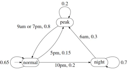
Example 4.17 We model the environment for the travel

example as in Fig. 4. The probabilities are chosen such that the long-run distribution is approximately(5

24, 11 24,

8 24) forpeak,normalandnightmode, respectively. The long-run distribution is based on the fact that peak hours are 6am-9am, 5pm-7pm (5 hours), normal hours are 9am-5pm and 7pm-10pm (11 hours), and quiet night time is 10pm-6am (8 hours). Note that there is no transition from peak hours to quiet time directly. The traffic will first reduce to normal and then to the night time.

4.3.2 Web services in environment

Given a versatile environment, the web services adapt themselves to fit in. The composition of the underlying models is of two-folds. At any state(𝑠, 𝑠)it is possible to have an environmental change or carry out a web ser-vice. Therefore, we stratify the model states into(𝑠, 𝑠) and(𝑠𝑀, 𝑠), where only environmental changes can take

place in the former states and only web service execution

Figure 4: Environment model

could take place in the later states. The resulting model is an MDP and is defined as follows:

Definition 4.18 Given a CWS MDP model _ =

(𝑆, 𝑠

0 , 𝐴, 𝐏,

_{, 𝐴𝑃}_{, 𝐿}_{) and the}

environ-ment model = (𝑆, 𝑠

0,𝐏), the composed model is an MDP|| = (𝑆, 𝑠₀, 𝐴,𝐏,_, 𝐴𝑃 , 𝐿), where

• 𝑆 = {(𝑠, 𝑡),(𝑠, 𝑡) ∣ 𝑠 ∈ 𝑆, 𝑡 ∈ 𝑆}, with 𝑠₀ = (𝑠₀ , 𝑠₀)as the initial state;

• 𝐴=𝐴∪ {𝑒𝑛𝑣}, where𝑒𝑛𝑣is a new action;

• 𝐏((𝑠, 𝑡), 𝑒𝑛𝑣,(𝑠, 𝑡′))=𝐏(𝑡, 𝑡′)and𝐏((𝑠, 𝑡), 𝛼,(𝑠′, 𝑡))= 𝐏(𝑠, 𝛼, 𝑠′);

• ((𝑠, 𝑡), 𝑒𝑛𝑣,(𝑠, 𝑡′)) = 0 and ((𝑠, 𝑡), 𝛼,(𝑠′, 𝑡)) =

(𝑠, 𝛼, 𝑠′);

• 𝐴𝑃 =𝐴𝑃, and𝐿((𝑠, 𝑡))=𝐿(𝑠).

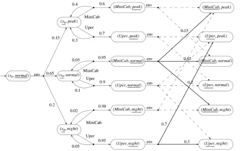
Example 4.19 Given the CWS MDP in Fig. 3 and the

en-vironment model in Fig. 4, the resulting MDP is shown in Fig. 5. Note that due to the space limit, we only show the part of the MDP (the first two steps from the CWS MDP). The model starts from the initial state (𝑠₀,normal) where a probability distribution (labelled with action𝑒𝑛𝑣)

takes place, which is from the statenormalin the environ-ment model. In the next level, from state(𝑠₀,peak), two actions are taken from the CWS MDP, but the probabili-ties are from the peak time availability𝑄₀in Table 3.

normal peak night

𝑄₀ 𝑄_𝑡(ℎ) 𝑄_𝑠 𝑄_𝑐(£) 𝑄₀ 𝑄_𝑡 𝑄_𝑠 𝑄_𝑐 𝑄₀ 𝑄_𝑡 𝑄_𝑠 𝑄_𝑐

MiniCab 0.95 0.9 0 50 0.6 1.7 0 57 0.98 0.68 0 49 Uper 0.9 0.9 0 40 0.7 1.7 0 51 0.95 0.68 0 26 Express 0.98 2 0 100 0.98 2 0 115 0.98 2 0 100

Local 0.9 5 2 50 0.85 5.5 2 60 0.91 5 2 50

Table 3: The QoS in different environment

The reward structure will depend on the environ-ment model and will only have positive rewards on transitions that start from CWS-active states, i.e., (𝑠, 𝑡). In this example, the travel time is 𝑄𝑡

(

(𝑠₀,night),

Uper,(Uper,night)) = 0.68ℎ, the number of transfers is

𝑄𝑠 (

(𝑠₀,night),Uper,(Uper,night))= 0, and the cost is

𝑄𝑐 (

(𝑠₀,night),Uper,(Uper,night))=£26.

4.3.3 Analysis

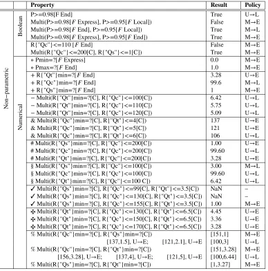
We now show the results of the running example against some typical properties listed in Table 4. We will explain what it means to the model and, in particular, how they can be used for the web service composition. The policies in the last column specify which CWSs to select and in which order.

Boolean results The boolean results tell whether a given

property is true or false.

• The first property in Table 4 - P>=0.98[F End] - is a reachability probabilityproperty. For all policies the probability of reaching B is no less than 0.98. An ex-ample policy is Uper𝑡𝑜Local.

• The next three areparetoproperties. When the journey is finished, either it is achieved by the express train or the local train, but not both (hence Multi(P>=0.98[𝐹

Express], P>=0.95[𝐹 local]) is false). A

counterexam-ple policy for the false property is given.

• The next two are related to rewards. The first one is areachability rewardproperty and the second one is a multi-objective referring to the expected total cumula-tive values.

Numerical results

• The first class of properties we compute is the (un-bounded) reachability probability. As it is an MDP, where uncertainty arises, it is to compute the maximum or minimum reachability probability. In Table 4, the minimum probability of reaching city B by an express train is 0. The maximum probability of arriving at B is 1.0, as the probability of taking a loop (whose probabil-ity is less than 1) infinitely many times is 0. See the∗ rows in Table 4.

• The second class of properties we compute is the reach-ability rewards. It is to compute the maximum or min-imum reward when reaching a certain goal. In Table 4, we listed three properties (rows marked with+) to cal-culate the minimum time, cost, number of stops when reaching City B (It takes 2 hours, £99.6 and 1 stop at the minimum. Note that this is the weighted mean average between different modes of the environment.

• The third class of properties issingle objective single constraint. It has one soft and one hard QoS require-ment. To study these properties, one way is to first fix a pair of QoS measures, say𝑄_𝑡(time) and 𝑄_𝑐 (cost),

and then change the bounds of the restriction (𝑄_𝑡 <= 2,2.3,3, etc) and see how the value of the other

prop-erty changes (minimum𝑄_𝑐 is £104, £99.3, £87.8,

spectively). As the travel time increases, the budget re-duces. See&marked in Table 4. The other direction also holds - when budget increases (£100, £110, £120), the travel time decreases (6.42, 5.75, 5.09 hours), see rows marked with−.

Figure 5: Concrete web service model and environment composition

shorter and the cost stays the same.

• The fourth class is a generalisation of the third class -single objective multiple constraints. It has one soft and multiple hard QoS requirement. In Table 4, it shows in✠that when the travelling time is no more than 3.5 hours and as the budget increases (£149, £150, £155), the minimum number of transfers reduces (1.09, 1.05, 1.00). This is expected as a higher budget means the affordability to take an express train. Similarly, the✠ -marked rows show the case when a minimum travel time is calculated for a restricted budget and time.

• The last class ismultiple objective properties. The re-sults contain the extreme points in the region. For in-stance, Multi(R{"Qc"}min=?[C], R{"Qs"}min=?[C]) has four extreme points. All the points included within the four points form a region where the two factors (cost and number of stops) are competing with each other.

Often one is not able to obtain a policy that can min-imise both objectives and has to compromise.

In summary, the QoS requirements from all aforemen-tioned classes can be checked. Either none of the exist-ing CWSs would satisfy the requirement and, if this is the case, a counterexample is given, or a policy on which CWSs to select and how to compose them is returned.

4.4

Web service composition via parametric

analysis

Property Result Policy

N

on

−

par

ame

tric

Boolean

P>=0.98[F End] True U→L

Multi(P>=0.98[𝐹Express], P>=0.95[𝐹 Local]) False M→E Multi(P>=0.98[𝐹End], P>=0.95[𝐹 Local]) True M→L

Multi(P>=0.98[𝐹Express], P>=0.95[𝐹 End]) True M→E

R{"Qc"}<=110 [𝐹End] False M→E

Multi(R{"Qc"}<=200[C], R{"Qs"}<=1[C]) True M→E

N

umer

ical

∗Pmin=?[𝐹 Express] 0.0 M→E

∗Pmax=?[𝐹 End] 1.0 M→E

+R{"Qt"}min=?[𝐹 End] 3.28 U→E

+R{"Qc"}min=?[𝐹 End] 99.6 M→L +R{"Qs"}min=?[𝐹End] 1 M→E

−Multi(R{"Qt"}min=?[C], R{"Qc"}<=100[C]) 6.42 U→L −Multi(R{"Qt"}min=?[C], R{"Qc"}<=110[C]) 5.75 U→L −Multi(R{"Qt"}min=?[C], R{"Qc"}<=120[C]) 5.09 U→L

&Multi(R{"Qc"}min=?[C], R{"Qt"}<=4[C]) 137 U→E &Multi(R{"Qc"}min=?[C], R{"Qt"}<=5[C]) 121 U→E

&Multi(R{"Qc"}min=?[C], R{"Qt"}<=6[C]) 106 U→L #Multi(R{"Qs"}min=?[C], R{"Qc"}<=200[C]) 1.00 U→E

#Multi(R{"Qc"}min=?[C], R{"Qc"}<=200[C]) 99.60 U→L #Multi(R{"Qt"}min=?[C], R{"Qc"}<=200[C]) 3.28 U→E

§Multi(R{"Qs"}min=?[C], R{"Qc"}<=100[C]) 3.00 M→L

§Multi(R{"Qc"}min=?[C], R{"Qc"}<=100[C]) 99.60 U→L

§Multi(R{"Qt"}min=?[C], R{"Qc"}<=100 C]) 6.42 U→L ✓Multi(R{"Qs"}min=?[C], R{"Qc"}<=99[C], R{"Qt"}<=3.5[C]) NaN –

✓Multi(R{"Qs"}min=?[C], R{"Qc"}<=130[C], R{"Qt"}<=3.5[C]) NaN –

✓Multi(R{"Qs"}min=?[C], R{"Qc"}<=155[C], R{"Qt"}<=3.5[C]) 1.00 M→E

✠Multi(R{"Qt"}min=?[C], R{"Qc"}<=130[C], R{"Qt"}<=6.5[C]) 4.45 U→E ✠Multi(R{"Qt"}min=?[C], R{"Qc"}<=150[C], R{"Qt"}<=6.5[C]) 3.36 U→E

✠Multi(R{"Qt"}min=?[C], R{"Qc"}<=170[C], R{"Qt"}<=6.5[C]) 3.28 U→E %Multi(R{"Qc"}min=?[C], R{"Qs"}min=?[C]) [151,1] M→E [137,1.5], U→E; [121,2.1], U→E [100,3] U→L

%Multi(R{"Qc"}min=?[C], R{"Qt"}min=?[C]) [151,3.28] M→E [156,3.28], U→E; [137,4], U→E; [121,5], U→E [100,6.44] U→L

%Multi(R{"Qs"}min=?[C], R{"Qt"}min=?[C]) [1,3.27] M→E

Table 4: Non-parametric Analysis Results for Travelling Example with Environment M – MiniCab, U – Uper, L – Local, E – Express

QoS requirement, which will be addressed by a parametric multi-objective analysis with the aid of the state-of-the-art probabilistic model checker PRISM.

4.4.1 Parametric environment and QoS models

As mentioned in Section 1, there are generally two oc-currences of parameters in our models, i.e., in the envi-ronment and in the QoS of web services. Fig. 4 gives an

example of the first case. The probability to go from nor-maltonight(peak) could be𝑝1(𝑝2) instead of0.2(0.15),

naturally, the probability to go fromnormal to itself is 1 −𝑝₁−𝑝₂. This probability parameters will remain to

composition, those QoS parameters continue to be QoS parameters in the resulting parametric MDPs. The follow-ing example introduces three parameters, two of which are the probabilities in the environmental model (𝑝₁, 𝑝₂) and

the last one is a QoS measure𝑞_𝑡.

Example 4.20 In this case study, we will have three

pa-rameters: 𝑝₁ ∈ [0.1,0.3] (the probability from normal to night), 𝑝₂ ∈ [0.1,0.4] (the probability from normal to peak) and 𝑞_𝑡 ∈ [0.6,2] (the average time to drive from home to train station). Note that 𝑞_𝑡 is introduced

as there is a high variation in the arriving time and the Uper/MiniCab fare closed related to𝑞_𝑡. Here we assume

the taxi fare𝑄_𝑐 is a linear function in𝑞_𝑡. Depending on

how jammed the traffic is, one would choose MiniCab or Uper to minimise the cost. The parametric QoS measures are set in Table 5. The other measures remain the same as in Table 3.

MiniCab Uper

𝑄_𝑡(ℎ) 𝑄_𝑐(£) 𝑄_𝑡(ℎ) 𝑄_𝑐(£)

normal 0.5𝑞_𝑡+ 0.3 34𝑞_𝑡+ 10 0.5𝑞_𝑡+ 0.3 3𝑞_𝑡+ 4

peak 0.5𝑞_𝑡+ 0.5 24𝑞_𝑡+ 22 0.5𝑞_𝑡+ 0.5 35𝑞_𝑡+ 9

night 0.4𝑞_𝑡+ 0.2 35𝑞_𝑡+ 7 0.4𝑞_𝑡+ 0.2 20𝑞_𝑡+ 2

Table 5: The parametric QoS in three environment modes

Probabilistic verification tools support automated solv-ing parametric MDPs against various kinds of properties specified before. (In probabilistic verification terms, they are unbounded until and reachability rewards properties.) Depending on the property under consideration, the re-sult is then given as either a rational function over the pa-rameters or as a mapping from regions of these papa-rameters to rational functions or truth values [39, 40]. To be more specific, given a property, we usually have three types of results which can be exploited for web service selection: it is either a boolean result, a numerical result of probabil-ities/rewards, or, in the presence of a parametric model, an explicit form of a rational function that can be optimised or plotted.

4.4.2 Parametric analysis

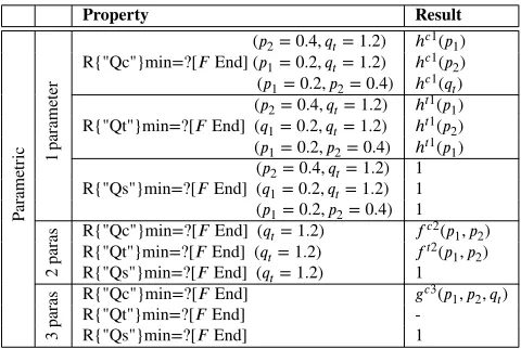
In the parametric analysis, it is possible to have one or more parameters the ranges of which are given. For a

reachability probability or a reachability reward property, the closed-form expressions for the objective could be cal-culated. For instance, we have described three parameters

𝑝₁ ∈ [0.1,0.3], 𝑝₂ ∈ [0.1,0.4], 𝑞_𝑡 ∈ [0.6,2] in Section 4.4. We are to show cases with 1, 2 and 3 parameters. The results are summarised in Table 6.

Property Result

Par

ame

tric 1par

ame

ter

R{"Qc"}min=?[𝐹End](𝑝₂= 0.4, 𝑞_𝑡= 1.2) ℎ𝑐1_(𝑝 1) R{"Qc"}min=?[𝐹End](𝑝1= 0.2, 𝑞𝑡= 1.2) ℎ𝑐1(𝑝2)

R{"Qc"}min=?[𝐹End] (𝑝₁= 0.2, 𝑝₂= 0.4) ℎ𝑐1_(𝑞 𝑡) R{"Qt"}min=?[𝐹End] (𝑝₂= 0.4, 𝑞_𝑡= 1.2) ℎ𝑡1_(𝑝

1) R{"Qt"}min=?[𝐹End] (𝑞₁= 0.2, 𝑞_𝑡= 1.2) ℎ𝑡1_(𝑝

2)

R{"Qt"}min=?[𝐹End] (𝑝1= 0.2, 𝑝2= 0.4) ℎ𝑡1(𝑝1)

R{"Qs"}min=?[𝐹End] (𝑝₂= 0.4, 𝑞_𝑡= 1.2) 1 R{"Qs"}min=?[𝐹End] (𝑞₁= 0.2, 𝑞_𝑡= 1.2) 1 R{"Qs"}min=?[𝐹End] (𝑝1= 0.2, 𝑝2= 0.4) 1

2

par

as R{"Qc"}min=?[𝐹End] (𝑞_𝑡= 1.2) 𝑓𝑐2_(𝑝 1, 𝑝2) R{"Qt"}min=?[𝐹End] (𝑞_𝑡= 1.2) 𝑓𝑡2_(𝑝

1, 𝑝2) R{"Qs"}min=?[𝐹End] (𝑞_𝑡= 1.2) 1

3

par

as R{"Qc"}min=?[𝐹End] 𝑔𝑐3_(𝑝 1, 𝑝2, 𝑞𝑡) R{"Qt"}min=?[𝐹End]

-R{"Qs"}min=?[𝐹End] 1

Table 6: Parametric Analysis Results for Travelling Ex-ample with Environment

One parameter If we instantiate the two parameters

𝑝₂= 0.4, 𝑞_𝑡= 1.2, that would leave only one parameter𝑝₁.

The function for the minimum cost is captured byℎ𝑐1(𝑝1),

where𝑐means it is to calculate the cost and1means there is one parameter. The function is of the following form for𝑝₁ ∈ [0.1,0.3]is shown in (1). The functionsℎ𝑐1_(𝑝

2)

andℎ𝑐1_(𝑞

𝑡)are in the similar fashion with𝑝2and𝑞𝑡as the

parameter, respectively.

ℎ𝑐1(𝑝1) =(145397874025𝑝21+ 117281115430𝑝1+ 2189373409209)

∕(244893675𝑝2₁+ 4572125610𝑝₁+ 21340212843)

(1)

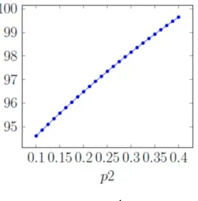
ℎ𝑐1(𝑝₂) =(36960320250𝑝3₂− 168561353275𝑝2₂

+776963615860𝑝₂+ 1932464456940)

∕(136890075𝑝2₂+ 3382066380𝑝₂+ 20889704748)

(2)

Figure 6:ℎ𝑐1_(𝑝 1)

When the functions are plotted, we can see how the three parameters are related to the minimum expected cost of reaching City B, respectively.

Figure 7:ℎ𝑐1(𝑝₂)

It shows from Table 3 that it is cheaper to travel in the night than at normal time. As a result, when𝑝₁increases,

the price drops, and that explains the trend in Fig. 6. On the contrary, it costs more to travel at the peak time. Thus when more weights are towards the peak time, i.e.,𝑝₂

in-creases, the cost would rise, see Fig. 7. As the MiniCab or Uper fare is positively linearly related to𝑞_𝑡, it means that

when𝑞_𝑡increases the taxi cost also increases, see Fig. 8.

With the closed-form expression, it is possible to evaluate the value (in this case the minimum cost) given the value to the parameter. For instance,ℎ𝑐1(𝑝₁) = £101.04when instantiating𝑝₁= 0.2in Eq. (1).

Figure 8:ℎ𝑐1(𝑞_𝑡)

Two parameters If the model has two parameters, the

resulting closed-form expression could be quite involved. Let’s still take the minimum cost𝑄_𝑐 as the objective and

let𝑞_𝑡= 1.2.

The function𝑓𝑐2_(𝑝

1, 𝑝2)calculates the minimum cost

when parameters𝑝₁∈ [0.1,0.3]and𝑝₂∈ [0.1,0.4].

𝑓𝑐2(𝑝₁, 𝑝₂)

=(66121292250𝑝2₁𝑝₂+ 98870908500𝑝₁𝑝2₂+ 36960320250𝑝3₂

+118949357125𝑝2₁− 246838623450𝑝₁𝑝₂− 188335534975𝑝2₂

+200197219450𝑝₁+ 823686488860𝑝₂+ 1887667038765)

∕(244893675𝑝2₁+ 366188550𝑝₁𝑝₂+ 136890075𝑝2₂

+4425650190𝑝₁+ 3308828670𝑝₂+ 19994778963)

Given this closed-form expression, we can evaluate the function𝑓𝑐2_{(0.1,0.1) = 95.75, which means that when}

the probability to go from normal to night and from nor-mal to peak are both 0.1, then the minimum expected cu-mulative value of total cost (𝑄_𝑐) is £95.75. The plot can

be found in Fig. 9.

Likewise we can have a similar analysis on how two parameters vary to affect the measure𝑄_𝑡(time to reach B).

The different combinations of parameters can be found in Fig. 10 and 11.

Three or more parameters. When there are more than