Variable Singularity Power Wedge Element for
Multilayered Composites
Ugo Icardi
*, Federico Sola
Dipartimento di Ingegneria Meccanica e Aerospaziale, Politecnico di Torino, Italy *Corresponding Author: [email protected]
Copyright © 2014 Horizon Research Publishing All rights reserved.
Abstract
Multilayered composites can be weakened by local failures, which can give rise to singular stress fields. Singularities can be removed or integrated to obtain bounded quantities which may be used for the analysis. In any case, the participation of singular stresses should be identified. Serving this purpose, a new mixed singular wedge element based on interpolation functions with a variable singularity power is developed, which can adapt to the problem and can represent the non-singular fields as a particular case. The displacements and the interlaminar stresses are assumed as nodal d.o.f. to a priori fulfill the kinematic and stress contact conditions at the material interfaces and the stress boundary conditions in point form. The application to sample cases taken from literature shows that the element can be successfully employed for the analysis of singular fields. The variable singular representation and the mixed formulation give more accurate results than their displacement-based, non-singular, or singular counterparts with a fixed singularity. The failure loads of initially delaminated specimens are accurately predicted either using the virtual crack closure technique or a mesoscale model by running in a reasonable time on a personal laptop computer.Keywords
Stresses Singularity, Singular Finite Element, Mixed Formulation, Crack Damage, Delamination, Laminated Composites1. Introduction
Multilayered composites are increasingly finding use, owing to excellent strength and stiffness-to-weight ratios, long fatigue life and advantageous energy absorption properties. As their performances can be weakened by local failures (e.g., fibre breakage, intralaminar and interlaminar matrix cracking, fibre/matrix debonding, delamination), an accurate prediction of their residual strength and stiffness is mandatory. A recent comprehensive review of the mechanisms of damage formation and evolution and of their modeling is given by Ivañez and Sanchez [1], Hassan et al.
[2], Tay et al. [3], Càrdenas [4], Liu and Zheng [5] and Hongkarnjanakul et al. [6].
Damaged areas require a full three-dimensional analysis, since the out-of-plane stresses, usually negligible elsewhere, have a significant bearing on keeping equilibrium in these regions and determine the stress singularities rise at matrix and delamination crack tips. As extensively discussed by Ebrahimi et al. [7] and Koguchi and da Costa [8], a different order of the singularity power is determined by the geometry and the constituent materials. The singular stress fields can be (i) removed or (ii) integrated to arrive at bounded quantities which can be physically interpreted and used for the analysis of progressive damage evolution and failure (see Berthelot [9] and Liu and Zheng [10]). Case (i) is that of continuum damage mesomechanics (CDM), while case (ii) is that of fracture mechanics (FM). Approach (i) is easy to implement into the finite elements and treats crack initiation and growth within a unified model. Approach (ii) is nowadays widely employed to predict the delamination growth using the virtual crack closure technique (VCCT) to solve the energy release rates (ERR). As examples, the papers by Okada et al. [11], Leski [12] and Liu et al. [13] are cited. If not experimentally determined, the critical ERR are computed by criteria such as those by Benzeggagh and Kenane [14], Wu and Reuter [15] and Reeder et al. [16].
Usually, finite element models are used as structural models, since closed form approaches should be limited to the analysis of certain range of geometries and loading conditions, due to the simplifying assumptions adopted, while shear-lag approaches, variational methods and stress transfer mechanics use parameters that should be determined by experiments.
interpolation functions with singular derivatives [34]-[36]. Progressive refinements have been brought to these techniques, in order to ensure compatibility of the crack-tip singular elements with the standard elements without using transition bridging elements. In this way it is possible to weaken the consistence requirements for the field functions, allowing to use certain discontinuous displacements and to develop more efficient ways to construct the stiffness matrix.
For a crack lying close to a bi-material interface like in laminated composites, the stress singularity is oscillating in nature, i.e. σij≈r-1/2+ic while for a crack perpendicularly terminating at the interface the stress field is of the form
σij≈rλ-1 (0<λ<1). In the previous formulas r is the radial
distance from the crack tip, λ is the lowest root of the characteristic equation, ricis the oscillatory term due to the mismatch in elastic properties of the two bonded material. Therefore, an arbitrary order of singularity should be embedded in the elements. Elements with variable singularity power have been recently developed using different approaches and successfully applied for solving different problems in the papers by Zhou et al. [37] and Chen et al. [38]. In [37] a three-dimensional variable-order boundary element with variable singularity order and different kinds of displacement formulations was suggested, while in [38] a special five-node singular triangular crack-tip element with extra basis functions in the G space and strain smoothing was proposed.
In the present paper, a solid singular, mixed wedge element for analysis of composite laminates is developed. It uses simple singular interpolation functions with variable singularity power that can degenerate into a non-singular standard representation as a particular case. This element is developed assuming the displacements and the out-of-plane stresses (i.e., the interlaminar stresses) as nodal d.o.f, since in this way, it a priori fulfills kinematic and stress contact conditions at the material interfaces, which are essential for keeping equilibrium, and it easily satisfy the stress boundary conditions in a point form. This element, which can be particularized as a displacement based element, is compatible with the standard ones (solid trilinear displacement based elements and non-singular mixed elements). The mixed formulation is chosen because it can provide more accurate results than displacement-based models with the same meshing and with a comparable processing time. The element is developed considering displacement and stress interpolating functions all of the same order, therefore the equilibrium is satisfied in an approximate integral form. The interpolation functions by Hughes and Akin [39] are used for the displacements, giving rise to singular derivatives with a variable singularity power that can be set as desired and can represent the regular (i.e. non-singular) behavior as a particular case. The interpolation functions for the nodal stresses are obtained deriving those for the displacements with respect to the coordinate that lies in a plane parallel to the layers where delamination/debonding cracks can rise and consequently a
singularity line rises at the crack tip. Satisfaction of equilibrium in approximate integral form assuming a unique set indifferently for the displacement or the stress d.o.f. components is a simplification that does not result in an accuracy loss, as shown by Nakazawa [40]. More accurate stresses than with displacement-based elements are obtained with the same meshing, along with an improved convergence rate. The present element is employed around the delamination crack singularity, while to ensure compatibility with no need of transition elements, the non-singular brick elements with the same d.o.f and standard three-linear interpolating functions developed by Icardi and Atzori [41] and extensively applied to analysis of composites are used elsewhere. Due to the interpolation scheme with quasi-standard features, the element can be easily implemented into the computer code [41] and used to account for the effects of singularities. The present solid modeling will result in an increase of data preparation and processing time with respect to plate models customarily adopted for the analysis of composite laminates, but simplifying assumptions will not be introduced across the thickness that could limit accuracy, as discussed, e.g., by Weißgraeber and Becker [42]. So the present modeling can be more accurate with arbitrary geometries, lay-ups, loading and boundary conditions and the crack growth mechanism can be easily simulated by splitting the interfaces. The accuracy of the present modeling will be assessed considering sample test cases with singular stress fields taken form the literature and initially delaminated specimens, for which experimental results are available, whose failure loads will be predicted using fracture mechanics and a mesomechanic approach. In the former case, the analysis of delamination will be carried out using the singular representation, as in the papers by Ariza et al. [43] and Yao and Hu [44]. In the latter case, the regular behavior will be set by removing the effects of the singularity, similarly to McQuigg [45].
The numerical results will show that the failure loads of initially delaminated specimens are accurately predicted with an affordable effort for a personal laptop computer either using the virtual crack closure technique, or a mesoscale model. Correct results are obtained with a relatively coarse meshing, thanks to the possibility to adapt the singularity power and owing to the improved accuracy of the mixed formulation. Of course, more accurate results are obtained when the singularity power is appropriately set and the regular behavior can be correctly predicted by setting the singularity power to zero. The displacement-based elements particularized from the mixed elements give less accurate predictions.
2. The wedge Element
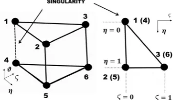
Figure 1 represents the wedge element in its natural volume of coordinates (η, θ, ζ) and in physical coordinates
parallel to that of the constituent layers, with x, η in the spanwise direction and y, θ in the transverse direction, as a consequence, z and ζ lie in the thickness direction. The displacements and the interlaminar stress components are indicated as u, v, w, σxz, σyz, σzz, respectively. The axes x and
[image:3.595.90.268.219.322.2]y are required to lie in a plane parallel to the constituent layers, while z is required to lie in the thickness direction, so that the singular line from nodes 1 to 4 lies on an interface. Distorted elements with a reduced distance from the nodes 1 and 4 can be constructed in order to approximate a point singularity.
Figure 1. The wedge element in its natural volume and numbering of nodes
2.1. Interpolation Scheme
The displacements and the interlaminar stresses are interpolated separately as:
D =
∑
61
De e disp
N
; S =∑
61
Se e stress
N
(1)The symbols Ne
disp, Nestress represent the interpolation functions for the displacements and the stresses, which are here indicated by D and S, respectively:
{D | S}T =
{
}
Tzz yz xz
w
v
u
,
,
|
σ
,
σ
,
σ
(2) Their corresponding nodal values, which represent the nodal d.o.f. of the present element, are indicated as:{De| Se}T =
=
{ }
q
( )e T=
{
e i e i e i eu v w
, ,
,
σ
xzi e,
σ
yzi e,
σ
zzi}
T (3) It is desirable that the interpolation functions have a variable stress singularity power that can adapt to the problem, in order to treat all constituent materials, geometries, loading and boundary conditions. The interpolation functions should also be able to represent the regular behavior, in order to obtain a conventional element as a particular case. Here, the shape functions with singular derivatives developed by Hughes and Akin [39] are used for interpolating the displacements:(
−η
β)
ϑ
= 1 1 dispN (4)
(
ζ
)
ϑ
η
β−
=
1
2
disp
N
(5)ζϑ
η
β=
3
disp
N
(6)(
−
η
β)
(
−
ϑ
)
=
1
1
4
disp
N
(7)(
ζ
)(
ϑ
)
η
β−
−
=
1
1
5
disp
N
(8)(
ϑ
)
ζ
η
β−
=
1
6
disp
N
(9)The stresses are instead interpolated by differentiating the previous functions with respect to the coordinate ζ, which is supposed to lie in a plane parallel to the layers where delamination/debonding can rise:
(
−
η
µ)
ϑ
=
1
1
stress
N
(10)(
ζ
)
ϑ
η
µ−
=
1
2
stress
N
(11)ζϑ
η
µ=
3
stress
N
(12)(
−
η
µ)
(
−
ϑ
)
=
1
1
4
stress
N
(13)(
ζ
)(
ϑ
)
η
µ−
−
=
1
1
5
stress
N
(14)(
ϑ
)
ζ
η
µ−
=
1
6
stress
N
(15)In this way, the stresses become singular at η =0, i.e. along the edge connecting nodes 1 and 4, with a singularity power μ≡ β - 1 that can adapt to the problem under investigation. The regular behavior is obtained by setting
β= 1 in (4) to (9) and assuming μ= 1 in (10) to (15).
As shown by Kaneko and Padilla [46], elements based on the shape functions defined above could have a convergence rate depending on the location of the interpolation points. Namely, locations can exist in which they could not work. However neither the present numerical applications, nor other authors have shown the occurrence of such prejudicial effects in the practical cases examined.
It could be noticed that equilibrium is fulfilled in an integral form, because (18) does not always produce intra-element self-equilibrating stresses. As mentioned in the introductory section, this representation is chosen because it simplifies the development of the element and does not have detrimental effects on accuracy.
As all the stresses should have the same singularity power, though they can have different singularity strength, the interpolation functions (10) to (15) are used for representing the inner variation also of the in-plane stress components. The element matrix and the vector of equivalent nodal forces are derived in a straightforward way by the Hellinger-Reissner mixed variational principle:
1 2 0
u
HR ij ij ij ijkl kl i i i i
V V St
HR HR
C dV bu dV t u dS
U W
δ δ σ ε σ σ δ
δ δ
∏ = − − + =
= − =
∫
∫
∫
(16)displacements and stresses given above. Please note that, the symbol bi represents the volume forces, ui represents the displacements of the points where these forces are applied, ti are the surface tractions, εu
ij=½(ui,j + uj,i) represent the strains derived from the strain-displacement relations (the differentiation with respect to the physical coordinates is indicated by a comma), while σ kl are their counterparts obtained with the stress-strain relations:
{ } (
{
11 12 13 14 15 16)
;T
ij C xx C yy C xy C xz C yz C zz xx
σ
ε = σ + σ + σ + σ + σ + σ σ
(
C21σxx+C22σyy+C23σxy+C24σxz+C25σyz+C26σzz)
σyy;(
C31σxx+C32σyy+C33σxy+C34σxz+C35σyz+C36σ σzz)
xy; (17)(
C41σxx+C42σyy+C43σxy+C44σxz+C45σyz+C46σ σzz)
xz;(
C51σxx+C52σyy+C53σxy+C54σxz+C55σyz+C56σ σzz)
yz;(
61 62 63 64 65 66)
}
T
xx yy xy xz yz zz zz
Cσ +C σ +C σ +C σ +C σ +C σ σ
The stresses are represented as:
}
{
{
}
{
}
{
}
{
}
{
}
{
}
}
{
{
}
{
}
{
}
{
}
{
}
}
{
{
}
{
}
{
}
{
}
{
}
{ }
( ) ˆ0 0 0 0 0
0 0 0 0 0
0 0 0 0 0
stress e stress stress D N q N N σ = (18)
the matrix [Dˆ] being obtained from the relation that defines
the in-plane stress components
{
}
[ ][ ]
*
{ }
( )ˆ
{ }
( )T
xx yy xy
S B q
eD q
eσ σ σ
=
=
(19)by inserting zeros in the appropriate positions. Since the interlaminar stresses σxz, σyz, σzz are assumed as nodal d.o.f., the interfacial stress contact conditions are a priori fulfilled when the nodes lie over a material interface. Though the continuity of the transverse normal stress gradient σzz,z, which is also prescribed by the elasticity theory, and the boundary conditions σzz,z = 0 at the upper and lower bounding faces cannot be enforced with the chosen d.o.f., they are spontaneously met, as observed by Icardi and Atzori [41] and by the present results. The present wedge
element can be connected at nodes 2,3,5,6 to the non-singular hexahedral element by Icardi and Atzori [21], which has the same nodal d.o.f. and compatible tri-linear interpolation functions.
Singular and non-singular displacement-based counterpart elements can be particularized from the present wedge element, which is referred as W6-MX-SG, according to the scheme of Table 1. In the numerical applications, the results by the present element will be compared to those of its counterpart elements defined in Table 1, in order to show the advantages of the mixed formulation and the variable singularity power representation.
As customarily, a topological transformation is carried out from the physical volume (x, y, z) to the natural volume
(η, θ, ζ) to uniform the computation of the volume integrals.
This operation transforms any wedge element into the prismatic element of Figure 1, i.e. the nodal displacements eui, evi, ewi and the stresses eσi
xz, eσiyz, eσizz into their counterparts e
ηui, eθvi, eζwi, eσiηζ, eσiθζ, eσiζζ in the natural volume. To this purpose, the coordinates of the internal points are expressed in terms of the nodal coordinates through the standard tri-linear interpolation functions Nj
c obtained from the Nj
disp of (4) to (9) by setting β= 1:
)
,
,
(
)
,
,
(
61 j j j
j
c
x
y
z
N
z
y
x
=
∑
(20)The derivatives with respect to the physical coordinates are computed as:
1
,
,
,
,
T T
x y z
η ϑ ζ
−
∂ ∂ ∂
∂
∂
∂
= ℑ
∂ ∂ ∂
∂
∂
∂
(21)|
ℑ
| being the Jacobian of the transformation1 1 1 2 2 2
1 2 3 4 5 6
3 3 3
1 2 3 4 5 6
4 4 4
1 2 3 4 5 6
5 5 5 6 6 6
, , , , , ,
, , , , , ,
, , , , , ,
c c c c c c
c c c c c c
c c c c c c
x y z x y z
N N N N N N
x y z
N N N N N N
x y z
N N N N N N
x y z x y z
η η η η η η
ϑ ϑ ηϑ ϑ ϑ ϑ
ζ ζ ζ ζ ζ ζ
ℑ =
(22)
Table 1. Elements that can be particularized from the present element and from [41]
Element name Type d.o.f Interpolation Singularity power
W6-MX-SG mixed displacements and stresses singular variable
W6-MX mixed displacements and stresses non-singular ---
W6-SG displacement-based displacements singular variable
W6 displacement-based displacements non-singular ---
B8-MX [41] mixed displacements and stresses non-singular ---
[image:4.595.90.522.613.740.2]In the numerical applications, the element matrix and the vector of the nodal forces will be derived using symbolic calculus, as in this way they are generated once at a time for all the elements. With this approach, the integrals involved in Eq. (16) will be computed in a closed form, thus avoiding the possible numerical instabilities due to Gaussian integration.
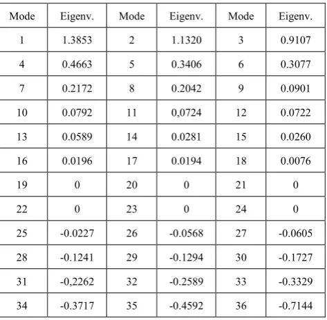
The readers are referred to Hoa and Feng [47] for a comprehensive discussion of stability and solvability of mixed elements. Summing up, for being admissible, these elements should have a number of displacement d.o.f. that is larger or equal to that of stress d.o.f., but certain choices of the interpolation functions could not yield meaningful results. An eigenvalue test performed over a single finite element with unit length edges, which is free of boundary conditions, should be carried out to ensure admissibility. Instead, a sufficient condition for solvability requires that the number of zero eigenvalues of the stiffness matrix should be equal to the number of rigid body modes, that the number of positive eigenvalues should be equal to the number of stress d.o.f., while the total number of zero and negative eigenvalues should correspond to the number of displacement d.o.f.
[image:5.595.61.298.493.725.2]An isotropic material with unit elastic moduli and a Poisson’s ratio of 0.3, should be used in order to have eigenvalues with the same magnitude. The successful results of this test over the element W6-MX-SG and its particularizations (because the results coincide in the test case) is shown in Table 2, while those for the element B8-MX are shown in the paper by Icardi and Atzori [41]. Hereafter, the virtual crack closure technique and a damage mesomodel used for predicting the delamination failure loads will be briefly reviewed.
Table 2. Solvability test for the present singular wedge element
Mode Eigenv. Mode Eigenv. Mode Eigenv.
1 1.3853 2 1.1320 3 0.9107
4 0.4663 5 0.3406 6 0.3077
7 0.2172 8 0.2042 9 0.0901
10 0.0792 11 0,0724 12 0.0722
13 0.0589 14 0.0281 15 0.0260
16 0.0196 17 0.0194 18 0.0076
19 0 20 0 21 0
22 0 23 0 24 0
25 -0.0227 26 -0.0568 27 -0.0605
28 -0.1241 29 -0.1294 30 -0.1727
31 -0,2262 32 -0.2589 33 -0.3329
34 -0.3717 35 -0.4592 36 -0.7144
2.2. Virtual Crack Closure Technique
Efficient ways for computing the energy release rates (ERR), which represents the drive force, since the crack propagates when they exceed a critical value, are based on the VCCT, as discussed in a comprehensive review by Krueger [48]. It is assumed that a crack propagates from a node i, which is split into two nodes whose relative displacements in the three directions are indicated as Δisx,
Δisy, Δisz. The nodal forces before propagation are indicated by Fix, Fiy, Fiz. The sole assumption of VCCT is that the energy required for a crack propagation Δα is equal to that required to close two separate crack surfaces of the same length Δα. The total ERR due to the crack propagation G is expressed as the sum of the ERR corresponding to the three modes GI, GII, GIII, i.e. the opening (mode I), the forward shearing or sliding (mode II) and the anti-plane tearing or scissoring (mode III) modes:
0 0
0 0
1
lim ( ) ( )
2
( ) ( ) ( ) ( )
a
i i a
a a
i i i i
G F x a sx a da
F y a sy a da F z a sz a da
∆
∆ →
∆ ∆
= ∆ +
Σ
+ ∆ + ∆
∫
∫
∫
(23)
Σ being the area generated by the crack propagation Δα. Usually, the so called two-step method is employed for computing G, because it can be successfully used with a not extremely refined meshing. This method uses the node forces before crack propagation and the node relative displacements after crack propagation:
1
( )
2
i i i i i i
G
=
F x sx F y a sy F z sz
∆
+
∆
+
∆
Σ
(24)As an alternative, the one-step method could be used, which however requires a refined meshing. It considers coupled the displacements of nearest nodes before crack propagation, instead of the relative displacements after crack propagation.
The meshing should be chosen by considering the balance between accuracy and computational efficiency and by doing also convergence rate considerations, because a too refined meshing can result disadvantageous by the viewpoint of convergence, as shown by Krueger [48]. Under mode I, usually accuracy is not appreciably improved by refining the discretization, while it is improved of a small percentage under mixed modes (see Liu et al. [13]). Here the meshing size is chosen by stopping the refinement when precision is incremented less than 5 %. The following criteria, widely used for the analysis of delamination via VCCT, are employed for estimating the equivalent critical ERR of mixed-modes:
B-K law (Benzeggagh and Kenane [14])
η
+ +
+ −
+ =
III II I
III II cr
I cr II cr I cr
equiv G G G G GG G G
G ( ) (25)
0 a cr III III a cr II II a cr I I cr equiv
G
G
G
G
G
G
G
G
m n
+
+
=
(26)Reeder law (Reeder et al. [16])
( )
( )
cr cr cr cr II III equiv I II I
I II III
cr cr III II III III II
II III I II III
G G
G G G G
G G G
G G G
G G
G G G G G
η η + = + − + + + + + − + + + (27)
where Gcr
I, GcrII and GcrIII represent the critical ERR for modes I, II and III. The choice of the exponents can determine quite different results, as observed by Liu et al. [13] and in the present numerical applications. The values 0.5, 1 and 2 have been used in literature, but the most accurate results are obtained with the latter two values. 2.3. Damage Mesoscale Model
This model considers an intermediate scale between that of the laminate and the micro-scale of the mechanisms of damage. Matrix microcracking, local delamination, diffuse damage and diffuse delamination are efficiently described by replacing the discretely damaged medium with an equivalent continuous homogeneous medium, which is equivalent to the damage micromodel from an energy standpoint and can simulate structures of industrial complexity. The behavior is described by means of two mesoconstituents, the single layer and the interface, which represents the thin layer of matrix between two adjacent plies. The damage state of each mesoconstituent is quantified by damage variables linked to the loss of stiffness of the mesoconstituent, whose evolution depends on damage forces that represent the variation of the energy with respect to the damage. These damage variables are assumed constant across the thickness of each mesoconstituent, but can vary changing the mesoconstituent.
The damage mesoscale model (DMM) by Ladevèze et al. [49] is employed in this paper. In summary, the displacement, strain and stress fields representing the exact micro-solution are represented as SM =S͂ + S̅, S͂ being the solution of the problem with the damage removed and S̅ the solution of a residual problem where each cracked area is loaded by the residual stress σ̴͂. Damage indicators are introduced, which are defined as the integrals of the strain energy for any basic residual problem. The strain energy Ej
p of the interface γj is expressed as:
3 33 3 2 23 2 1 13 1
~
)
~
1(
~
)
~
1(
~
)
~
1(
2
k
I
k
I
k
I
E
j jp
σ
σ
σ
γ
+
−
+
−
+
−
=
(28)where k͂1, k͂2 and k͂3 are the elastic stiffness coefficients of the interface and I̅1, I̅2 and I̅3 the damage indicators, which depend just on the material properties of the
mesoconstituent layer. They can be conveniently computed by a 3-D finite element analysis, as shown by Ladevèze and Lubineau [50], since the damage state of a ply depends on the state of damage of the adjacent plies. To this purpose, in this paper a cell subjected to the residual stresses is discretized by non-singular wedge elements, assuming the stiffness of the interface equal to the shear modulus of the matrix divided by its thickness, which is assumed as the thickness of a ply divided by 5. The progressive failure analysis by DMM is carried out at each increment of displacement or loading by evaluating the homogenized stresses at any point and comparing them to the strength. Damage is extended to the points where the ultimate strength is reached.
3. Numerical Assessments
3.1. Two-Material Wedge
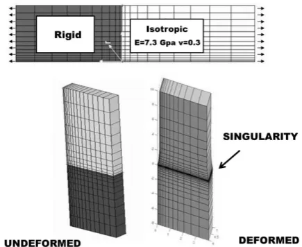
[image:6.595.323.541.507.685.2]As a first test, the sample case of a two-material wedge is considered (Figure 2). Many studies have been published since the 60’s for this or similar cases, where analytical solutions have been presented. The exact elasticity solution by Hein and Erdogan [51] and the eigenvalue analysis by Yamada and Okumura [52] show that a singularity due to the dissimilar properties of the interfaced materials rise at the corner interface for certain side angles. The singularity power for this case considerably varies with geometry and material properties. With a mild variation of the properties and side angles of 60° or less there is no stress singularity, while for larger angles and dissimilar materials a strong singularity rises. The largest singularity power corresponds to the case with an interface angle of 90° when one of the materials is rigid.
Figure 2. Geometry, loading and meshing for the two-material wedge problem
as this represent the most severe case. The problem was simulated subdividing the domain into 600 elements, 275 of which in the rigid sector and 325 in the elastic sector, with a progressive refinement along the interface and at the left corner (Figure 2), where the results are compared to the reference solution. Around this corner, 30 singular wedge elements were used. A Young’s modulus of 7.3 GPa and a Poisson’s ratio of 0.3 were assumed for the deformable sector, while a modulus larger by a factor 100 was assumed for simulating the rigid sector. The variation of the ratio of the elastic moduli of the two sectors produces the variation of the singularity power shown in Figure 3. A singularity power α=0.22 corresponds to the case with an interface angle of 90° and one of the materials rigid. This value was found by a log-linear procedure, because a straight line is shown in the stress vs. distance log-log plot at the right α for each case with different elastic ratios and side angles. The exponent μ that appears in the interpolation functions is related to the singularity power by:
µ
β
α
=
1
−
=
(29) then the singular stress field is represented as:)
(
− +1−
+
ℜ
ℜ
=
κ
α ασ
ij ijO
(30)ℜ
being the radial distance from the singularity,κ
ij the singularity strength and O(ℜ
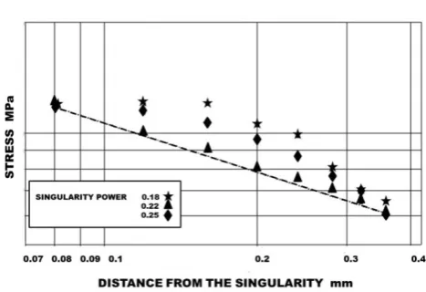
-α+1) negligible higher-order terms. Figure 4 shows the curves obtained in the log-log plots when α≠
0.22 and the straight line corresponding to [image:7.595.316.550.87.247.2]α=0.22. Table 3 reports the results when the singularity power is incorrectly set to 0.5 (symbol *) or it is set to 0 and thus represents the non-singular case (symbol °). It is evident from these results that the interpolation functions with variable singularity power give more accurate predictions. Forward and in the next Section, other cases with different singularity powers are considered, in order to assess the accuracy of the present finite element simulation.
Figure 3. Variation of the stress singularity power α with the ratio of the
elastic moduli of the two sub-domains
Figure 4. The log-linear procedure used for setting the exponent of interpolation functions
[image:7.595.312.551.523.685.2]Figure 5 shows the results with a crack at the tip. The variation of the stress singularity power with the ratio of the elastic moduli in the two sub-domains is shown for a Poisson’s ratios of 0.2 of the elastic sector, this case being also considered by Hein and Erdogan [51] and Yamada and Okumura [52]. To enable a comparison with the results reported in [52], the characteristic equation used to solve the eigenvalue problem was reconstructed in the finite element model simulation by work-conjugating the nodal stresses to the strains obtained from the nodal values of displacements and the interpolation functions, in a region around the corner interface. In this way, it was possible to compute the eigenvalue λ, which is related to the singularity power α since α=|1-λ|, (the symbol | | was used to indicate the modulus). The results of Figures 3 and 5 and Table 3 show that the solution by the present finite element model is free from spurious modes; it gives accurate predictions of the singular behavior and can correctly determine the real and imaginary parts of the eigenvalue λ.
[image:7.595.64.298.524.693.2]Table 3. Singularity power of the two material wedge problem by setting a different singularity power in the interpolation functions
Analysis (+) by: log (E
1m/E2m)=1 log (E1m/E2m)=2 log (E1m/E2m)=3
W6-MX-SG+B8-MX 0.130 (0.134)° (0.145)* 0.198 (0.203)° (0.212)* 0.213 (0.216)° (0.237)*
W6-SG+B8 0.135 (0.138)° (0.151)* 0.192 (0.189)° (0.203)* 0.209 (0.205)° (0.216)*
EXACT 0.131 0,195 0.214
(+) eigenvalue analysis
3.2. L-Shaped Region
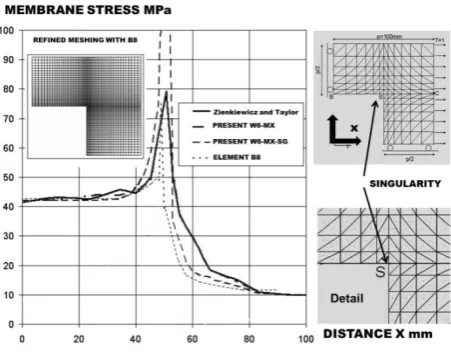
As a further test, it is now considered the L-shaped plane geometry represented in Figure 6, where a stress singularity is generated by the opening corner (point S). The reference solution for this case is represented by the finite element analysis with non-singular displacement-based triangular plate elements by Zienkiewicz and Taylor [53].
Figure 6. L-shaped region: variation of the in-plane stress σxx with the
distance from the opening corner S
In the present analysis, the problem was discretized considering a single layer of solid elements. Four singular wedge elements were used around the opening corner (point S), while 213 regular wedge elements were used elsewhere. The reference solution [53] shows that, approaching the corner singularity along the line B-C, σxx becomes about eight times greater than far from it. A similar result is obtained by the present finite element model when the regular behavior is set in the wedge elements around the opening corner, non-singular elements being used in the reference solution. In Figure 6 also the results obtained using displacement based elements B8 are reported. The comparison of these results to those by the mixed elements W6-MX-SG and W6-MX shows that even with refining meshing, elements B8 always give less accurate results. This result confirms the well-known fact that hybrid and mixed elements are more accurate than displacement-based elements with the same meshing. Figure 7 shows that the results by the present finite element simulation are still in a
[image:8.595.314.549.267.439.2]very good agreement with the exact solution by Hein and Erdogan [51] and the eigenvalue analysis by Yamada and Okumura [52] for this case. Forward, applications will be presented to laminates.
Figure 7. Singularity eigenvalue analysis for the L-shaped region
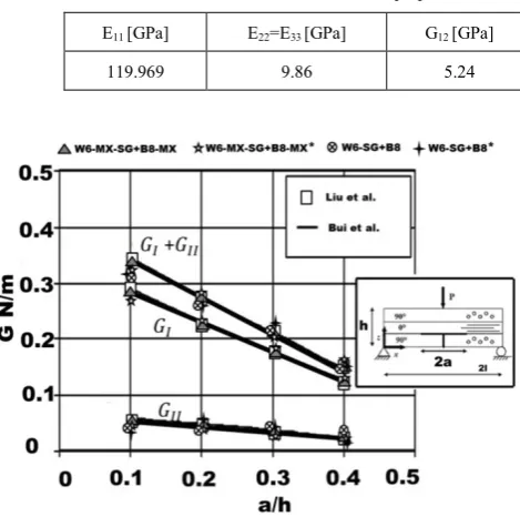
3.3. Assessment of the Fracture Mechanics Model Now a simply-supported (90°5/0°5/90°5) cross-ply beam under a point centered loading is considered to the purpose of assessing whether the implementation of the fracture mechanics model was correct. The beam has a transverse crack in the matrix and an interfacial delamination at the upper interface of the intermediate layer. The beam is 2.187 mm thick and has a length of 50.8 mm, the constituent materials have the properties reported in Table 4 and the loading has a magnitude P=13.345 N.
For this case, the results by Liu et al. [54] and Bui et al. [55] are available for comparisons. The width was chosen large enough to avoid the interaction among the stresses from the free edge and those due to the delamination crack.
[image:8.595.67.293.305.482.2]Table 4. Material properties used in the tests of the fracture mechanics model
E11 [GPa] E22=E33 [GPa] G12 [GPa] G13=G23 [GPa]
υ
12υ
13= υ
23119.969 9.86 5.24 5.24 0.3 0.3
Figure 8. Variation of the energy release rates GI , GII and GI +GIIwith the
ratio a/h of the delamination crack half-length with respect to the thickness
The results by Liu et al. [54] and Bui et al. [55] reported in Figure 8 show the variation of the strain energy release rates GI and GII separately and their sum GI+GII as a function of the ratio a/h, a being the half length of the delamination crack and h the thickness of the beam. The results by the present finite element model reported in this figure were obtained either by setting the singularity power to 0.5 to enable a comparison with [54] and [55], or setting it with the log-linear procedure. Either displacement-based elements that can be particularized by the mixed elements, as shown in Table 1, or the wedge and brick mixed elements were considered in the analysis. The results of Figure 8 show that the strain energy release rates are correctly computed by the present finite element simulation. However, also in this case the most accurate predictions are still obtained by the mixed elements and when the singularity power is set by the log-linear procedure. Once shown the finite element model to be accurate and the fracture mechanics model correctly implemented, delaminated specimens will be analyzed. These new tests will also serve as assessments of the damage mesoscale model.
3.4. Initially Delaminated Specimens
The following sample cases are considered, whose experimental failure loads are known:
Case A. Double cantilever unidirectional beam made of AS4-3K/PEI layers under mode I;
Case B. Double cantilever angle-ply beam made of XAS/931C layers under mode I;
Case C. Angle-ply end-loaded split beam made of T400/6376C layers under mode II;
Case D. End-notch-flexure cross-ply beam made of AS4-3501-6 layers under mode II.
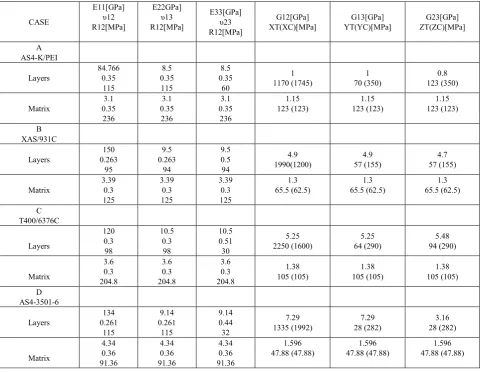
Case A. This case refers to a beam made of 16 unidirectional layers aligned in the 0° direction, each 0.22 mm thick, whose properties are given in Table 5. The beam is 146.5 mm long; it has a width of 20.0 mm and a thickness of 3.52 mm. A centered non-stick film 59 mm long and 15 μm thick is interposed at the symmetry plane interface, in order to give rise to an initial delamination. GIcrit was determined by Fassine and Pavan [56] as 1.841 KJ/m2 and the experimental failure load as 74.94 N. The delamination load for this case is reported in Table 6. The computations were carried out discretizing the beam into 30, 10 and 16 solid elements in the spanwise, width and thickness directions, respectively, with a progressive refinement at the tip where 15 wedge elements were used.
The results show that a more accurate prediction is obtained by VCCT when the proper singularity power is set, than with setting the non-singular behavior or a singularity power of 0.5. Since the failure occurs as a matrix failure under traction, the contributions by GII and GIII are negligible, thus the propagation criteria (25) and (27) are reduced to Gcr
equiv = GcrI, while (26) becomes Gequiv/Gcr =
(GI /GcrI), consequently just αm =1 has meaning.
The damage mesoscale model (DMM) by Ladevèze et al. [49] also provides results in a good agreement with the experiment carrying out the homogenization process by the finite element model using as strength the matrix strength under traction and setting the non-singular behavior in the wedge elements.
Table 5. Material properties of initially delaminated specimens
CASE
E11[GPa] υ12 R12[MPa]
E22GPa] υ13 R12[MPa]
E33[GPa] υ23 R12[MPa]
G12[GPa]
XT(XC)[MPa] YT(YC)[MPa] G13[GPa] ZT(ZC)[MPa] G23[GPa]
A AS4-K/PEI
Layers 84.766 0.35
115
8.5 0.35 115
8.5 0.35
60
1
1170 (1745) 70 (350) 1 123 (350) 0.8
Matrix 0.35 3.1
236
3.1 0.35 236
3.1 0.35
236
1.15
123 (123) 123 (123) 1.15 123 (123) 1.15
B XAS/931C
Layers 0.263 150
95
9.5 0.263
94
9.5 0.5 94
4.9
1990(1200) 57 (155) 4.9 57 (155) 4.7
Matrix 3.39 0.3
125
3.39 0.3 125
3.39 0.3 125
1.3
65.5 (62.5) 65.5 (62.5) 1.3 65.5 (62.5) 1.3
C T400/6376C
Layers
120 0.3 98
10.5 0.3 98
10.5 0.51 30
5.25
2250 (1600) 64 (290) 5.25 94 (290) 5.48
Matrix
3.6 0.3 204.8
3.6 0.3 204.8
3.6 0.3 204.8
1.38
105 (105) 105 (105) 1.38 105 (105) 1.38
D AS4-3501-6
Layers 0.261 134
115
9.14 0.261
115
9.14 0.44 32
7.29
1335 (1992) 28 (282) 7.29 28 (282) 3.16
Matrix
4.34 0.36 91.36
4.34 0.36 91.36
4.34 0.36 91.36
1.596
47.88 (47.88) 47.88 (47.88) 1.596 47.88 (47.88) 1.596
VCCT appears advantageous over DMM as it does not require additional costs due to the homogenization process, while the singular representation offers the capability to predict presence and nature of singularities at the same costs of the non-singular representation. However, in this case an accurate prediction of the failure load can be obtained also using stress-based criteria (the results by Chang-Springer’s [57] and Davila-Camanho’s [58] criteria are reported) if the stresses
σ͂ij computed by setting the non-singular behavior are averaged over a distance from the crack tip equal to the thickness of the laminate.
Case B. The beam is made of XAS/931C layers, each 0.125 mm thick, with the material properties reported in Table 5 and a [-45°/0° (45°)2/0°/(-45°)2/0°/45°]2 lay-up. The beam has a length of 150 mm, a width of 30 mm and a thickness of 3 mm. A Teflon film with a length a0 =29 mm and a thickness of 10 μm is interposed at the mid-plane to generate an initial delamination. Due to the 3-D stress field, delamination in this case occurs as a combination of the three modes. Robinson and Song [59] found an experimental failure load of 87 N for this case and numerically estimated Gcrit = 0.35 KJ/m2. The results by the present finite element model are still reported in Table 6. The beam was discretized by 30, 10 and 21 solid elements in the spanwise, width and thickness directions, respectively. The meshing was refined at the crack tip where the wedge elements were used, while the brick elements were used in the other regions. Also in this case 15 wedge elements were used. The mounting bulks bonded to the edges in order to apply the opening loading were discretized, as they represent a local increment of stiffness. The critical ERR for the three single modes were numerically estimated as suggested by Robinson and Song [59].
The results show that the propagation criteria (25)-(27) determine a different failure load with a different choice of the exponents (the law (26) was applied using equal exponents), as well as the important role played by the singularity power assumed in the interpolation functions. As shown by comparison with experiments, the results obtained with the singularity power set to 0 or 0.5 are again less accurate than those obtained setting the proper value with the log-linear procedure.
Table 6. Failure loads of initially delaminated specimens [N] and computational time {}; λ1 variable singularity power; λ2 singularity power=0.5; λ3
singularity power=0. DMM: Damage mesoscale model [49]; C-S: Chang and Springer’s criterion [57]; D-C: Davila and Camanho’s criterion [58]
CASE
A
B
C
D
Experiment
74.94 87.0 150.0 1192
VCCT
Law (25) {208 sec} {343 sec} {441 sec} {375 sec}
exp=0.5
λ1 74.72 75.2 125.32 1013.20
exp=2
λ1 74.72 81.1 141.58 1108.56
exp=1 λ1
λ2
λ3
74.72 73.22 70.98
86.43 84.70 82.32
144.21 141.33 138.02
1117.15 1094.62 1035.53 VCCT
Law (26) {210 sec} {345 sec} {443 sec} {376 sec}
exp=0.5
λ1 (no meaning) 73.64 117.48 1006.76
exp=2
λ1 (no meaning) 80.04 145.12 1126.08
exp=1 λ1
λ2
λ3
74.70 73.31 70.95
85.56 83.04 80.12
148.51 145.23 139.77
1153.62 1108.75 1104.28 VCCT
Law (27) {212 sec} {349 sec} {446 sec} {379 sec}
exp=0.5
λ1 74.72 73.52 126.40 1060.88
exp=2
λ1 74.72 75.36 140.34 1107.51
exp=1 λ1
λ2
λ3
74.72 73.22 70.98
86.23 84.20 80.59
146.88 139.57 135.81
1173.52 1072.58 1146.07
DMM 73.58 {206 sec} 86.35 {338 sec} 146.96 {436 sec} 1175.93 {368 sec}
C-S 71.60 {202 sec} 80.82 {332 sec} 142.15 {428 sec} 1091.18 {363 sec}
D-C 74.51 {203 sec} 81.31 {334 sec} 147.26 {429 sec} 1108.29 {365 sec}
The processing time is reported in Table 6 also for this case leaving apart the generation of the element matrices and the homogenization process.
In this case, the Chang and Springer’s and Davila and Camanho’s criteria predict failure loads that are comparable each other and to the experimental load only if the stresses
σ͂ij are averaged over a distance from the delamination crack tip at least of 4 mm, which is larger than in the previous case. Please notice that numerical tests have shown that these criteria give monotonically increasing failure loads increasing the distance from the crack tip at which the stresses are evaluated, so they can overestimate the failure load at a sufficiently large distance if stress averaging is uncorrected.
mounting bulks were discretized and the critical ERR were still numerically estimated. As usual, wedge elements were used at the crack tip, whereas brick elements were used in the other regions.
The results show that the choice of the exponents of the propagation criteria produce larger variations than in the previous sample case, since the contributions by modes II and III are much more important. As shown by Table 6, the best results by VCCT were obtained by using the exponent 1 with all the propagation criteria, but good results were also obtained by using the exponent 2, while the exponent 0.5 gave inaccurate predictions. Again, the most accurate results were obtained by setting the singularity power with the log-linear procedure.
DMM still predicted a failure load in good agreement with VCCT and with the experiment, computing again the matrix failure through the rule by Davila and Camanho. The stress-based criteria still can provide accurate results considering the stresses computed using non-singular elements if these stresses are correctly averaged. The Davila and Camanho’s and Chang and Springer’s criteria predicted failure loads in a well agreement with the experiment when the stresses σ͂ij were averaged over a distance of about 6 mm from the crack tip, while the Choi-Chang’s delamination criterion used for a comparison required just a distance equivalent to the thickness of a ply.
The computational time again shows that the present analysis is affordable by a personal computer. However, it is presumed that a refined meshing should be used to more accurately determine the participation of the crack tip stresses for this case.
Case D. The latter case examined is that of an end-notch-flexure cross-ply beam under mode II, with a [(0°10/90°/0°10)/0°/90°/(0°10/90°/0°10)] lay-up, a length of 38.1 mm, an overall thickness of 5.1 mm and a width of 16.5 mm. Each constituent layer is 0.116 mm thick and has the properties reported in Table 5 (material AS4-3501-6). A Teflon film is interposed at the mid-plane during manufacturing, in order to simulate an initially delaminated area of length 19.05 mm. Kim and Sun [61] found an experimental failure load of 1192 N and the critical strain energy release GII crit =0.515 KJ/m2. Each constituent layer was discretized by a layer of elements, i.e. 44 elements were used across the thickness and the width was discretized by 5 elements, while 30 elements with a progressive refinement at the crack tip were used in the span direction. Table 6 shows that the results by VCCT are now very sensitive to the choice of the exponents of the propagation criteria. Still better results are obtained by setting the proper singularity power of wedge elements at the crack tip with the log-linear procedure. Also in this case accurate results are computed by the DMM model carrying out the homogenization process by finite elements and using the Davila and Camanho’s criterion. Application of the Davila and Camanho’s and Chang and Springer’s criteria using the stresses σ͂ij provided by the finite element analysis with the regular behavior shows that accurate
results are obtained averaging the stresses over a distance of 5 mm from the crack tip. It is shown that also in this case the computational time is affordable by a personal computer.
4. Concluding Remarks
A new mixed singular wedge element with a variable singularity power that can adapt to the problem and can represent the non-singular behavior as a particular case was developed for analysis of damaged composites. The accuracy of the element was initially assessed considering sample cases with singular stress fields due to dissimilar properties of materials, geometry or cracks, for which analytical solutions are available for comparisons. The numerical results proved that the present finite element simulation with mixed singular wedge elements around singularities and solid mixed elements elsewhere accurately predicts the presence and the nature of singularities, the related stress fields, the participation of the singular stresses and the regular behavior with an affordable computational effort for a laptop computer. The variable singular representation and the mixed formulation gave better results than their displacement-based, non-singular, or singular counterparts with a fixed singularity, confirming the results in literature. The failure loads of initially delaminated beams were computed using the virtual crack closure technique, a damage mesoscale model and comparisons were also made using stress-based criteria. The virtual crack closure technique was carried out setting the singular behavior with the appropriate singularity power in the wedge elements, while for the damage mesoscale model and the stress-based criteria the non-singular behavior was set. The comparison with experiments proved that accurate predictions can be obtained using fracture mechanics, but nearly equally accurate results can be obtained using damage mesomechanics and even stress-based criteria with an appropriate averaging of stress, as claimed in literature. The homogenization process required by the damage mesomechanics model, resulted in an additional cost for the damage mesoscale model. The results of the fracture mechanics model were sensitive to the exponents employed for estimating the critical energy release rates by the propagation criteria. The stress-based criteria required the stresses to be averaged over an appropriate distance from the tip, which appeared case dependent
REFERENCES
[1] I. Ivañez, S. Sanchez-Saez. Numerical modelling of the
low-velocity impact response of composite sandwich beams with honeycomb core, Composite Structures, Vol. 106, 716-723.
[2] M.A. Hassan, S. Naderi, A.R. Bushroa. Low-velocity impact
damage of woven fabric composites: Finite element simulation and experimental verification, Material & Design, Vol.53, 706-718.
[3] T.E. Tay, G. Liu, V.B.C. Tan, X.S. Sun, D.C. Pham.
Progressive failure analysis of composite, J. Compos. Mater., Vol.42, No.18, 1921-1966.
[4] D. Càrdenas, H. Elizalde, P. Marzocca, F. Abdi, L.
Minnetyan, O. Probst. Progressive failure analysis of thin-walled composite structures, Composite Structures, Vol.95, 53-62.
[5] P.F. Liu, J.Y. Zheng. Recent developments on damage
modeling and finite element analysis for composite laminates: A review, Materials & Design, Vol.31, No.8, 3825-3834.
[6] N. Hongkarnjanakul, C. Bouvet, S. Rivallant. Validation of
low velocity impact modelling on different stacking sequences of CFRP laminates and influence of fibre failure. Composite Structures, Vol.106, 549-559.
[7] S.H. Ebrahimi, S. Mohammadi, I. Mahmoudzadeh Kani. A
local PUFEM modeling of stress singularity in sliding contact with minimal enrichment for direct evaluation of generalized stress intensity factors, Eng. Fracture Mech., Vol. 105, 16-40.
[8] H. Koguchi, J.A. da Costa. Analysis of the stress singularity field at a vertex in 3D-bonded structures having a slanted side surface, Int. J. of Solids and Structures, Vol. 47, No. 22-23, 3131-3140.
[9] J.M. Berthelot. Transverse cracking and delamination in
cross-ply glass-fiber and carbon-fiber reinforced plastic laminates: static and fatigue loading, Appl. Mech. Rev. Vol.56, No.1, 111-147.
[10] P.F. Liu, J.Y. Zheng. Recent developments on damage
modeling and finite element analysis for composite laminates: a review, Material & Design, Vol.31, No.8, 3825-3834.
[11] H. Okada, H. Kawai, T. Tokuda, Y. Fukui. Fully automated
mixed mode crack propagation analyses based on tetrahedral finite element and VCCM (virtual crack closure-integral method), Int. J. of Fatigue, Vol.50, 33-39.
[12] A. Leski. Implementation of the virtual crack closure
technique in engineering FE calculations, Finite Elem. Anal. Des., Vol.43, No.3, 261-268.
[13] P.F. Liu, S.J. Hou, J.K. Chu, X.Y Hu, C.L. Zhou, Y.L. Liu,
J.Y. Zheng, A, Zhao, L. Yan. Finite element analysis of post-buckling and delamination of composite laminates using virtual crack closure technique, Composite Structures, Vol.93, No.6, 1549-1560.
[14] M. Benzeggagh, M. Kenane. Measurement of mixed-mode
delamination fracture toughness of unidirectional glass/epoxy composites with mixed mode bending apparatus, Compos. Sci. Technol., Vol.56, No.4, 439-449.
[15] E.M. Wu, R.C. Reuter Jr. Crack extension in fiber-glass
reinforced plastics, Ill TAM Report No. 275, 1965.
[16] J. Reeder, S. Kyongchan, P.B. Chunchu, D.R. Ambur.
Post-buckling and growth of delamination in composite
plates subjected to axial compression, 43rd
AIAA/ASME/ASCE/AHS/ ASC Structures, Structural Dynamics, and Materials Conference, 2002.
[17] G.B. Sinclair. Stress singularities in classical elasticity-I: removal, interpretation and analysis, Appl. Mech. Rev., Vol.57, No.4, 251-297.
[18] X. Hu, W. Yao. Stress singularity analysis of multi-material wedges under anti-plane deformation, Acta Mechanica Solida Sinica, Vol.26, No.(2), 151-160.
[19] J. Qian, N. Hasebe. On the technique of shifting side nodes in isoparametric elements to impose arbitrary singularity. Computers & Structures, Vol.66, No.6, 814-846.
[20] R.S. Barsoum. Triangular quarter point elements as elastic
and perfectly-plastic crack tip elements. Int. J. for Num. Meth. in Eng., Vol.11, pp.85-98.
[21] M. A. Jimenez, A. Miravete. Application of the finite-element method to predict the onset of delamination growth. J. Compos. Mater., Vol.38, No.15, 1309-1335.
[22] R.S. Barsoum. A degenerate solid element for linear fracture analysis of plate bending and general shells, Int. J. for Num. Meth. in Eng., Vol.10, 551-64.
[23] S.L. Pu, M.A. Hussian, W.E. Sorensen. The collapsed cubic
isoparametric element as a singular element for crack problems, Int. J. for Num. Meth. in Eng., Vol.12, 1727-1742. [24] R.S. Barsoum. On the use of isoparametric finite elements in linear fracture mechanics, Int. J. for Num. Meth. in Eng., Vol.10, 25-37.
[25] R. Wait. Finite element methods for elliptic problems with
singularity, Computational Methods for Applied Mechanics in Engineering, Vol.13, 141-150.
[26] H.D. Hibbit. Some properties of singular isoparametric
elements, Int. J. for Num. Meth. in Eng., Vol.11, 180-184. [27] L.A. Ying. A note on the singularity and the strain energy of
singular elements, Int. J. for Num. Meth. in Eng., Vol.18, 31-39
[28] L.-A. Ying. Some interpolation formulae of triangular and
quadrilateral elements, Int. J. for Num. Meth. in Eng., Vol.18, 959-966.
[29] M. Okabe, N. Kikuchi. Semi-radial singularity mapping
theory for line singularities in fracture mechanics, Comput. Meth. in Appl. Mech. and Eng., Vol.36, 257-276.
[30] G. C. Sih, H. Liebowitz. Mathematical theories of brittle
fracture. Fracture, An advanced treatise, Academic Press, New York, 1968.
[31] P.C. Paris, G. C. Sih. Stress analysis of cracks. Fracture
Toughness Testing and its Applications, ASTM STP 381, 1965.
[32] S. S. Pageau, S. B. Biggers. Enrichment of finite elements
[33] S. E. Benzley. Representation of singularities with isoparametric finite elements. Int. J. for Num. Meth. in Eng., Vol.8, 537-545.113
[34] D.M. Tracey, T. S. Cook. Analysis of power type singularities using finite elements, Int. J. for Num. Meth. in Eng., Vol.11, 1225-1233.
[35] M. Stern, E. Becker. A conforming crack tip element with
quadratic variation in the singular field, Int. J. for Num. Meth. in Eng., Vol.12, 279-288.
[36] M. Stern. Families of consistent conforming elements with
singular field, Int. J. for Num. Meth. in Eng., Vol.14, 409-421.
[37] W. Zhou, K.M. Lim, K.H. Lee, A.A.O. Tay. A new
variable-order singular boundary element for calculating stress intensity factors in three-dimensional elasticity problems, Int. J. Solids and Structures, Vol.42, 159-185.
[38] L. Chen, G.R. Liu, K. Zheng, J. Zhang. A novel variable
power singular element in G space with strain smoothing for bi-material fracture analyses, Eng. Anal. with Boundary Elements, Vol.35, 1303-1317.
[39] T.J.R. Hughes, J.E. Akin. Techniques for
developing ’special’ finite element shape functions with particular reference to singularities, Int. J. for Num. Meth. in Eng., Vol.15, No.5, 733-751.
[40] S. Nakazawa. Mixed finite elements and iterative solution
procedures. Iterative Methods in Non-Linear Problems. Pineridge, 1984.
[41] U. Icardi, A. Atzori. Simple, efficient mixed solid element for accurate analysis of local effects in laminated and sandwich composites, Advances in Eng. Software, Vol.32, No.2, 843-849.
[42] P. Weißgraeber, W. Becker. Finite Fracture Mechanics
model for mixed mode fracture in adhesive joints, Int J. of Solids and Structures, Vol.50, No.14-15, 2383-2394.
[43] M.P. Ariza, A. Sàez, J. Dominguez. A singular element for
three-dimensional fracture mechanics analysis, Eng. Anal. with Boundary Elements, Vol.20, 275-285.
[44] W.A. Yao, X.F. Hu. A novel singular finite element of
mixed-mode crack problems with arbitrary crack tractions, Mechanics Research Communications, Vol.38, 170-175
[45] T.D. McQuigg. Compression After Impact experiments and
analysis on honeycomb core sandwich panels with thin face sheets. Report no. NASA/CR–2011-217157, NASA Langley Research Center Hampton, USA, 2011
[46] H. Kaneko, P.A. Padilla. A note on the finite element
method with singular basis functions, Int. J. for Num. Meth. in Eng., Vol. 45, No.4, 491-495.
[47] S.V. Hoa, W. Feng. Hybrid finite element method for stress
analysis of laminated composites, Dordrecht: Kluwer, 1998.
[48] R. Krueger. Virtual crack closure technique: history,
approach, and applications, NASA/CR-2002-211628, ICASE Report No.2002-10.
[49] P. Ladevèze, G. Lubineau. D. Marsal. Towards a bridge
between the micro- and mesomechanics of delamination for laminated composites, Compos. Sci. Technol., Vol.66, No.6, 698-712.
[50] P. Ladevèze, G. Lubineau. On a damage mesomodel for
laminates: micromechanics basis and improvement, Mech of Materials, Vol.35, No.8, 763-775.
[51] V.L. Hein, F. Erdogan. Stress singularities in a two-material wedge, Int J of Fract Mech, Vol.7, No.3, 317-330.
[52] Y. Yamada, H. Okumura. Finite element analysis of stress
and strain singularity eigenstate, in Inhomogeneous Media or Composite Materials, Hybrid and Mixed Finite Element Methods, S.N. Atluri, R.H. Gallagher, O.C. Zienkiewicz, Ed. John Wiley & Sons Ltd, UK, 1983.
[53] O.C. Zienkiewicz, R.L. Taylor. The finite element method,
Ed. McGraw-Hill, New York, 1994.
[54] S. Liu, Z. Kutlu, F.K. Chang. Matrix cracking and
delamination in laminated composite beams subjected to a transverse concentrated line load, J. Compos. Mat., Vol.27, No.5, 436-470.
[55] V.Q Bui, E. Marechal, H. Nguyen-Dang, Imperfect
interlaminar interfaces in laminated composites: interlaminar stresses and strain energy release rates, Compos. Sci. Technol., Vol. 60, No.1, 131-143.
[56] R. Fassine, A. Pavan. Viscoelastic effects on the interlaminar fracture behavior of thermoplastic matrix composites: I rate and temperature dependence in unidirectional PEI/carbon fibre laminates, Compos. Sci. Technol., Vol.54, No.2, 193-200.
[57] F.K. Chang, G.S. Springer. The strengths of fiber reinforced composite bends, J. Compos. Mater., Vol.20, No.1, 30-47.
[58] C.G. Davila, P.P. Camanho. Failure criteria for FRP
laminates in plane stress, NASA/TM-2003-212663, 2003.
[59] P. Robinson, D.Q. Song. A modified DCB specimen for
Mode I testing of multilayered laminates, J of Compos. Mater., Vol.26, No.11, 1554-1577.
[60] N.S. Choi, A.J. Kinloch, J.G. Williams. Delamination
fracture of multidirectional carbon fiber/epoxy composites under mode I, mode II and mixed mode I/II loading, J Compos. Mater., Vol.33, No.1, 73-100.
[61] T.J., Kim, C.T. Sun. Influence of ply orientation on
![Table 1. Elements that can be particularized from the present element and from [41]](https://thumb-us.123doks.com/thumbv2/123dok_us/8756679.893042/4.595.90.522.613.740/table-elements-particularized-present-element.webp)
![Table 6. Failure loads of initially delaminated specimens [N] and computational time {}; λ1 variable singularity power; λ2 singularity power=0.5; λsingularity power=0](https://thumb-us.123doks.com/thumbv2/123dok_us/8756679.893042/11.595.65.546.94.563/failure-initially-delaminated-specimens-computational-singularity-singularity-lsingularity.webp)
