P h y si c al a n d n u m e r i c al
c o n s t r a i n t s in s o u r c e m o d e li n g
fo r fi ni t e d iff e r e n c e si m ul a ti o n of
r o o m a c o u s ti c s
S h e a ff er, J, v a n Wals tij n, M a n d F a z e n d a , B M
h t t p :// dx. d oi.o r g / 1 0 . 1 1 2 1 / 1 . 4 8 3 6 3 5 5
T i t l e
P h y si c al a n d n u m e r i c al c o n s t r ai n t s in s o u r c e m o d e li n g fo r
fini t e d iff e r e n c e si m u l a tio n of r o o m a c o u s ti c s
A u t h o r s
S h e aff er, J, v a n Wals tij n, M a n d F a z e n d a , B M
Typ e
Ar ticl e
U RL
T hi s v e r si o n is a v ail a bl e a t :
h t t p :// u sir. s alfo r d . a c . u k /i d/ e p ri n t/ 3 0 9 7 0 /
P u b l i s h e d D a t e
2 0 1 4
U S IR is a d i gi t al c oll e c ti o n of t h e r e s e a r c h o u t p u t of t h e U n iv e r si ty of S alfo r d .
W h e r e c o p y ri g h t p e r m i t s , f ull t e x t m a t e r i al h el d i n t h e r e p o si t o r y is m a d e
f r e ely a v ail a bl e o nli n e a n d c a n b e r e a d , d o w nl o a d e d a n d c o pi e d fo r n o
n-c o m m e r n-ci al p r iv a t e s t u d y o r r e s e a r n-c h p u r p o s e s . Pl e a s e n-c h e n-c k t h e m a n u s n-c ri p t
fo r a n y f u r t h e r c o p y ri g h t r e s t r i c ti o n s .
Physical and numerical constraints in source modeling for finite
difference simulation of room acoustics
a)Jonathan Sheafferb)
School of Computing, Science and Engineering, University of Salford, Salford, Greater Manchester M5 4WT, United Kingdom
Maarten van Walstijn
School of Electronics, Electrical Engineering and Computer Science, Queen’s University Belfast, Belfast BT7 1NN, United Kingdom
Bruno Fazenda
School of Computing, Science and Engineering, University of Salford, Salford, Greater Manchester M5 4WT, United Kingdom
(Received 1 July 2013; accepted 14 November 2013)
In finite difference time domain simulation of room acoustics, source functions are subject to various constraints. These depend on the way sources are injected into the grid and on the chosen parameters of the numerical scheme being used. This paper addresses the issue of selecting and designing sources for finite difference simulation, by first reviewing associated aims and constraints, and evaluating existing source models against these criteria. The process of exciting a model is generalized by introducing a system of three cascaded filters, respectively, characterizing the driving pulse, the source mechanics, and the injection of the resulting source function into the grid. It is shown that hard, soft, and transparent sources can be seen as special cases within this unified approach. Starting from the mechanics of a small pulsating sphere, a parametric source model is formulated by specifying suitable filters. This physically constrained source model is numerically consistent, does not scatter incoming waves, and is free from zero- and low-frequency artifacts. Simulation results are employed for comparison with existing source formulations in terms of meet-ing the spectral and temporal requirements on the outward propagatmeet-ing wave.
VC 2014 Acoustical Society of America. [http://dx.doi.org/10.1121/1.4836355]
PACS number(s): 43.55.Ka, 43.38.Ar, 43.55.Lb [LLT] Pages: 251–261
I. INTRODUCTION
The finite difference time domain (FDTD) method has
recently gained in applicability to room acoustics, largely owing to improved boundary formulations,1–4newly emerged schemes,5,6 and hardware-accelerated implementations.7–9 Among the various FDTD modeling aspects, grid excitation has received relatively sparse attention in the literature, with researchers in acoustics usually directly employing the methods inherited from their counterparts in the field of electromagnetics.
In FDTD simulation of electromagnetic fields, where the numerical scheme approximates a solution to Maxwell’s equations,10 a general distinction is made between a hard source (HS), which imposes a voltage or current on the elec-trical field, and a soft source (SS), which superimposes either variable onto the field.11,12By analogy, these forms of inject-ing energy into the grid can be used to simulate pressure and velocity sources in an acoustic field.
While in the first acoustic FDTD formulation by Botteldooren13 the field was excited by imposing velocity
across an area representing a speaker membrane, subsequent acoustic studies have often made use of omni-directional sources via HS or SS excitation at a single grid node. Similar source formulations can be found in the closely related simu-lation paradigm of digital waveguide modeling.14,15
One advantage of HS over SS excitation is that it allows a more precise control of the outward propagating pressure wave, which facilitates various modeling aims, such as field visualization and response analysis.16However, unlike with soft sources, waves propagating back to the source reflect from a hard source node,17 effectively imposing a severe limit on the available time window. Schneider and col-leagues18,19 addressed this major drawback by proposing
transparent sources(TS), which generate the same pressure
field as a HS but avoid the source node scattering by means of reflection cancellation; this involves measuring the grid impulse response prior to the principal numerical experi-ment, which carries a significant additional computational effort. A similarity between TS and the so-called total-field/scattered field and pure scattered field formulations was noted by Redondo and colleagues.20
More recently, Jeong and Lam21showed that HS and TS are prone to undesired low-frequency artifacts when certain excitation functions are used, and proposed the use of sine-modulated Gaussian pulses—which are not spectrally flat— to address this. In a similar vein, differentiated pulses have been in use in electromagnetic FDTD for some time, in order a)Portions of this work were presented in: “A physically-constrained source
model for FDTD acoustic simulation,” Proc. of the 15th Int. Conference on Digital Audio Effects (DAFx12), York, UK, September 2012.
b)
to avoid direct current (DC) flow excitation.11,12 These solutions exemplify the inherent trade-offs in FDTD source modeling, in this case balancing the elimination of low-frequency artifacts with effecting an outward wave of desira-ble frequency content. These findings also suggest that the methods for shaping and for injection of the source pulse should not be seen and chosen in isolation. The literature does not, however, give a clear view of how the various cri-teria relate to the underlying physics and the employed nu-merical formulations.
In order to obtain a broader insight into how trade-offs can be made in the design of acoustic FDTD source models, this paper addresses the problem by first reviewing the asso-ciated aims and constraints. Several methods for injection and pulse shaping are then evaluated against these criteria (Sec.III). In the following section, grid excitation modeling is generalized in the form of a digital filter chain, each filter representing a separate constraining system; this processing structure converts an arbitrarily chosen excitation signal into a final source function. Starting from a small pulsating sphere model, a new excitation method is then formulated by specifying suitable filters. Finally, the resulting physically constrained source (PCS) model is evaluated through numer-ical results and compared to existing methods in Sec.V.
II. THE FDTD METHOD IN ACOUSTICS
A. Yee-type method
The original FDTD method for electrodynamics sug-gested by Yee10makes use of two staggered grids represent-ing the electric and magnetic fields. In the field of acoustics, the method was adapted to solve Euler’s linearized equa-tions,13which represent propagation of pressure and particle velocity, and will be further referred to as aYee-type method.
When sources are present in the domain, the conservation laws of mass and momentum describing the sound field atx
¼(x, y, z)2R3, are given by22
1
c2
@pðx;tÞ
@t þq0r%uðx;tÞ ¼qðx;tÞ; (1)
q0
@uðx;tÞ
@t þrpðx;tÞ ¼F~ðx;tÞ; (2)
wherep(x,t) is sound pressure,u(x,t) is particle velocity,q0
is the ambient density of air, andcis the velocity of sound in air. Here, the functionq(x,t) denotes therate of fluid
emer-gencein the system in the dimension of density per unit time
(kg m&3 s&1), and the function F(x,~ t) is the acoustic force
exerted upon the source volume. For simplicity, it is assumed that all considered excitation functions represent volume velocity sources, and as such, the force term in Eq.
(2), is neglected. Accordingly, Eqs. (1) and (2) can be
approximated using finite difference operators as
dtpjni ¼ c2Tqj
n
i
|fflffl{zfflffl}
Source Term
&z0kðdxuxjni þdyuyjni þdzuzjniÞ (3)
and
dtuxjni ¼ & k
z0dx
pjni; (4a)
dtuyjni ¼ & k
z0d
ypjni; (4b)
dtuzjni ¼ & k
z0dz
pjni; (4c)
whereux,uy,anduzdenote the orthogonal components of the particle velocity vector uin a Cartesian coordinate system,
z0¼q0cis the characteristic impedance of air, andk¼cT/X
is theCourant number.23In the numerical domain, the sys-tem is sampled such that (x, y, z, t)![lX, mX, iX, nT] and accordinglynandi¼[l, m, i] are the index positions in dis-crete time and space, andXandTare, respectively, the spa-tial and temporal sample periods. The finite difference operators are given by
dtujni 'uj
nþ1=2
i &uj
n&1=2
i ; dtpjni 'pj
nþ1
i &pj
n
i; (5a)
dxujni 'uj
nþ1=2 lþ1=2;m;i&uj
nþ1=2
l&1=2;m;i; dxpj n
i'pj
n
lþ1;m;i&pj n l;m;i;
(5b)
dyujni 'uj
nþ1=2 l;mþ1=2;i&uj
nþ1=2
l;m&1=2;i; dypj n
i'pj
n
l;mþ1;i&pj n l;m;i;
(5c)
dzujni 'uj
nþ1=2 l;m;iþ1=2&uj
nþ1=2
l;m;i&1=2; dypj n
i 'pj
n
l;m;iþ1&pj n l;m;i:
(5d)
By direct substitution of Eq. (5) into Eqs. (3) and(4), and by removing any source terms, the update equations for air are obtained, as originally formulated by Botteldooren.13
B. Scalar wave equation method
While the Yee scheme is a popular choice of many authors, it is by no means the most efficient solution for room acoustics simulation.24In fact, if knowledge of particle velocity is not required throughout the entire soundfield, then one may employ a finite difference scheme approximat-ing the scalar wave equation for pressure, a formulation which is here referred to as the wave equation method.5
Accordingly, when sources are present in the domain, one considers the inhomogeneous wave equation,
1
c2
@2p
ðx;tÞ @t2 &r
2p
ðx;tÞ ¼wðx;tÞ: (6)
To enable a direct comparison with other studies, here
w(x,t) is defined as a general source driving function, whose physical relation to fluid emergence in the system shall be further discussed in Sec. III. Using the same nomenclature, the wave equation can be discretized as
ðd2
t &k2d2xÞpj
n
i ¼ c2T2wj
n
i
|fflfflfflffl{zfflfflfflffl}
Source Term
; (7)
with the finite difference operators given as
d2 tpj
n
i 'pj
nþ1
i &2pj
n
i þpj
n&1
d2 xpj
n
i 'pj
n
lþ1;m;i&2pj n l;m;iþpj
n
l&1;m;i; (9)
d2 ypj
n
i 'pj
n
l;mþ1;i&2pj n l;m;iþpj
n
l;m&1;i; (10)
d2zpj n
i 'pj
n
l;m;iþ1&2pj n l;m;iþpj
n
l;m;i&1; (11)
where the operatord2
xis given by
d2
x¼d
2 xþd
2 yþd
2 zþaðd
2 xd
2 yþd
2 xd
2 zþd
2 yd
2 zÞ þbd
2 xd
2 yd
2 z:
(12)
The free parameters a and b are chosen according to the desired properties of the numerical scheme being used. By setting a¼0, b¼0, applying the finite difference operators to Eq. (7), and removing the source term, one obtains the well known update equation for air in a rectilinear node arrangement.5
III. SOURCE MODELING REVIEW
A. General aims
In order to assess the merits and shortcomings of exist-ing source models, it is useful to review some of the require-ments for an idealized sound source in room acoustics simulation, which are generally similar to those of an acous-tic measurement. First, it is desired that the bandwidth of the source is wide enough to cover the entire frequency range of interest, and that it is sufficiently flat within that range.25,26 The sound source should generate a prescribed pressure field, meaning that one should be able to predict its magni-tude in free field. In many cases, it is useful to have a source that can excite the room omni-directionally at all frequencies of interest27(at least within the dispersion limitations of the numerical scheme). It is also important that the process of grid excitation is numerically consistent, meaning that a change in grid parameters would not affect the magnitude of the sound field generated by the source. Also, when transient phenomena are investigated, it is desired that the source ex-citation signal is sufficiently compact in time, so that tempo-ral overlap between discrete reflections is minimized. Last, although never feasible in a physical measurement, it is use-ful to be able to excite the room transparently, that is, with-out introducing scattering effects from the source itself.
B. Physical constraints
Equation (1)relates the time derivative of pressure and space derivatives of particle velocity to the rate of fluid emergence, q(x, t), which shall now be developed mathe-matically. In acoustics, a fundamental type of source known as a point monopole is a limitingly small object which radi-ates spherical wavefronts.28 Radiation could be caused, for example, due to a time-varying heat, or some mechanical force causing a sphere to pulsate and generate a volumetric flow (such a system will be described in more detail in Sec. IV A). In the limiting case, where the physical size of the object approaches zero, the soundfield at the source position, x0 ¼(x0, y0, z0) 2 R3 approaches a point of singularity in which the homogeneous wave equation is not satisfied. The
rate of fluid emergence inside a small volumeVsurrounding this point source must equal the local mass flow rate divided byV,
qðx;tÞ ¼q0QðtÞdVðx&x0Þ; (13)
whereQ(t) is the volumetric flow rate, or volume velocity of the source. In anticipation of how this applies to a discretized system in whichVis the volume occupied by a single FDTD node, it can be seen that Eq.(13), changes the dimension of volume velocity and, as such, presents a scaling constraint
relating the amplitude of the source to the volume it occu-pies. By combining Eqs. (2) and (1), the particle velocity vector is eliminated and the inhomogeneous wave equation is derived. It follows from this derivation and from the rela-tions described by Eq.(13), that the source term in Eq.(6), becomes
wðx;tÞ ¼@qðx;tÞ @t ¼
q0
V d
dtQðtÞdðx&x
0Þ: (14)
Physically, the quantity w(x,t) has the dimension of density per unit time squared (kg m&3s&2), and can be thought of as fluid emergence due to volume acceleration of the source.
Following Eq.(14), it can be seen that adifferentiation
constraintapplies to sources in the wave equation, meaning
that volume velocity should be injected as its first time deriv-ative. Observe that the source terms in Eqs.(1), and(6), are supplemental to the fundamental time-space relationships, that is, if one sets q(x, t)¼0 then the homogeneous wave equation is obtained. This indicates that fluid emergence is
an additive process, implying a superposition constraint,
which numerically means that source nodes should also be evaluated with the FDTD update equations for air.
In order to generate a volume velocity at the source, some mechanical system is required. Such a system would be governed by the laws of motion, and accordingly intro-duce further modeling constraints. While some mechanical constraints are specific to a chosen transducer, continuous DC flow is something that traditional acoustic transducers generally cannot produce, therefore one would expect that
ð1
&1wð
x;tÞdt¼0; (15)
which naturally occurs if the differentiation constraint
described in Sec.III Bis adhered to, and ifq(x,t) is compact in time (i.e., starts at and decays to zero within a finite amount of time). However, if one decides to arbitrarily choose
w(x,t), then failure to adhere to this constraint might have detrimental effects, as will be further discussed in Sec.V D.
C. Numerical constraints
frequencies prone to substantial dispersion, numerical errors contribute to the resulting response, which not only impair the ability to perform visual analysis, but may also introduce undesired audible artifacts in resulting auralizations.29
Accordingly, it is important that high frequencies are removed from the excitation signal to prevent these from contaminating the simulated field, which is here referred to
as abandwidth constraint.In the case of auralization, where
visual inspection of the soundfield is not required, the grid can be excited directly with the program material to be aural-ized. A more efficient way is to first determine the room’s impulse response using a unit impulse, and subsequently obtain the sound signals at the receiver locations via convo-lution. In such a case, bandlimiting can be enforced in the post-processing stage.
When transient phenomena are studied, the grid is excited with a short, impulsive source signal so that possible temporal overlap between reflections is minimized. Such a pulse signal is compact in time and as such can be said to adhere to a time-compactness constraint, which in practice has to be traded-off against the bandwidth constraint. Note that if the excitation signal is not finite in time by definition, it has to be truncated at points selected such that any discon-tinuity errors are minimal. In addition, the value of all of the signal derivatives up to the truncation order of the scheme would ideally also be zero at simulation onset. However, this further requirement has been reported to be prominent only for higher order numerical schemes.30
D. Injection methods
Most generally, an excitation signal can be injected via a single or multiple nodes into a grid representing any of the computed acoustic fields. As this paper aims to develop an excitation approach compatible with both Yee and wave equation schemes, further analysis and formulation will be given from the perspective of a single pressure node excitation.
1. Hard sources
A hard source is the simplest form of grid excitation, in which an acoustic quantity is directly imposed on the source node. This quantity is represented in the discrete domain by the excitation signalspjn, and accordingly, the update equa-tion for a HS node is
pjni0þ1¼spjnþ1; (16)
wherei0¼[l0,m0,i0] denotes the index position of the source. The first thing evident from Eq.(16), is that the laws of mass and momentum conservation are not satisfied at the source node, meaning that the HS does not adhere to a superposition constraint. In other words, update equations for air cannot operate over a HS node and any incoming waves get scattered by the source. Accordingly, the node is often loosely thought of as a sound radiating boundary node. This description, however, is not precise, as such an element should adhere to boundary conditions which are not evident in the HS formulation. In addition, one could argue that in a
real measurement scenario, a loudspeaker would inevitably be present in the room, and therefore scattering from a HS is not an unrealistic outcome. However, in an FDTD simula-tion the physical size of the sound radiating node is directly dependent on the spatial sample period, meaning that the scattering effects of the HS are numerically inconsistent.
2. Soft sources
The scattering and low-frequency problems21of hard sour-ces can be overcome by employing SS, in which the excitation signal is superimposed on a source node that has already been evaluated by the update equations for the medium. The update equation for a SS node on a pressure grid is therefore
pjni0þ1 ¼ pjni0þ1
n o
þspjnþ1; (17)
where fpjni0þ1g represents the result of updating the node with the general update equation for air, that is, Eq. (7), or
Eqs. (3), and (4), in the absence of any source terms. Soft
sources may have different effects depending on the type of scheme being used. In Yee-type grids, a SS is differentiated due to the staggered nature of the scheme. The update equa-tion for pressure progresses through time in only one half of a step, and the remaining half-step occurs when updating particle velocity, i.e., by evaluating the derivatives of pres-sure. This inherent differentiation is important as it ensures elimination of a DC component, yet it also severely modifies the spectrum of the outward propagating wave by generating a (normally undesired) roll-off in low frequencies.
In wave equation methods, the SS does not get auto-matically differentiated, and as such, gives a different result. The outward wave has a spectral content similar to that of
spjn, which is a desired feature. Because of this, however,
one is not free to arbitrarily choose the excitation signal. More specifically, any existing DC component in the excita-tion funcexcita-tion may cause the ambient pressure in the room to gradually increase. To explain this, let us consider a plane wave of arbitrary amplitude A propagating through the x -plane and interacting with a surface of reflection coefficient ^
r. The total sound pressure along the plane is given by
pðx;tÞ ¼Aejðxt&kxÞþ^rAejðxtþkxÞ: (18)
Accordingly, for x¼0 the sound pressure is uniformly
p¼A(1þr^) along the plane. Since the SS is being added to existing pressure, then for any^r>0 a pre-existing DC com-ponent would constructively superimpose on itself at the source node. This may result in an incremental offset in the response, as will be numerically evaluated in Sec. V D. Similar effects have been observed in the field of computa-tional electrodynamics.31
Based on digital waveguide analysis, Karjalainen and Erkut14identified the requirement to superimpose, differenti-ate and scale soft sources in wave equation FDTD schemes. Their formulation, which shall be further referred to as a
pjnl0þ;m10;i0¼ pj
nþ1 l0;m0;i0
n o
þq20AcX
w ð
Qjnþ1&Qjn&1Þ; (19)
where Aw denotes the cross-sectional area of the waveguide occupied by the source. Note that here the excitation function is explicitly defined as a volume velocity. The formulation adheres to both superposition and differentiation constraints, but being drawn from one dimensional (1D) waveguide theory the scaling factor would only be correct for 1D schemes.
3. Transparent sources
A side effect of all soft sources is that the injected exci-tation function is modified by the grid’s impulse response, which occurs due to the update equations for the medium operating over the source node.19 It is important to distin-guish between the effects of the grid’s impulse response, which have a minimal effect on the magnitude of the gener-ated soundfield and the differentiation process, which severely modifies the spectrum of the generated wave. Schneider and colleagues19 addressed some of these issues by making use of TS, which do not scatter incoming waves and do not get modified by the grid’s impulse response. The approach requires that the grid’s impulse response is meas-ured prior to the simulation stage and is compensated for during simulation. This process can be described mathemati-cally by
pjni0þ1¼ pjni0þ1
n o
þspjnþ1&
Xn
l¼0
Ijn&lþ1spjl; (20)
whereIjn denotes the pre-measured impulse response of the grid, which is obtained by exciting the grid with a unit impulse and capturing the result of updating the source node with the update equation for air.19 Therefore, TS in a Yee scheme do not only compensate for the grid’s impulse response, but also reverse the effects of source differentia-tion, effectively resulting in a sound field similar to that of a HS but without scattering any incoming waves. In addition, TS suffer from the same low-frequency artifacts as HS.21It should also be noted that the grid’s impulse response must be obtained in the absence of any scattering objects, which for long simulation times entails modeling a large domain and thus introduces an additional computational burden. In sum, it can be said that TS do not adhere to any scaling con-straints and, due to the grid compensation process, nor to the differentiation constraint.
E. Pulse shaping
The grid has to be excited with a pulse signal that adheres to the aforementioned bandwidth and the time-compactness constraints, and is usually defined in terms of a&6 dB cutoff frequency (fc) and the number of samples (M). Two widely employed pulse signals in FDTD modeling are the Gaussian pulse and the Blackman-Harris window.12 Figure1(a)shows the respective amplitude spectra for fc ¼ 0.1fs and M¼79. The Gaussian pulse signal has to be truncated with care in order to avoid the introduction of spectral ripples. The
Blackman-Harris pulse has inherent stopband ripples, and any detrimental effects may become particularly evident when lower cutoff frequencies are required.12
Differentiated versions of these pulse signals are some-times used in order to avoid DC excitation.11,12 A special case is the Ricker wavelet,32which is a normalized second-derivative of a Gaussian function, and has several docu-mented uses in acoustics FDTD.20,33,34In the light of the dis-cussion in Sec. III B, it can be said that the differentiation constraint is inherently met when using such pulses. Similarly, sine-modulated pulses12,21 have no DC compo-nent and may be considered as differentiated versions of pulse signals of finite power and length, thus also meeting the differentiation constraint. Figure 1(b) shows a spectral comparison between a Ricker wavelet, a differentiated Gaussian and a sine-modulated Gaussian.
It is worthwhile noting that the differentiation in Eq. (14), stems from the governing equations, which are discre-tized in the numerical formulation. It is therefore more con-sistent with the FDTD model to incorporate the source differentiation in the same discretized fashion, rather than performing an analytic differentiation on the initial pulse sig-nal. As explained in Sec. IV, this leads to the use of an “injection filter” for wave equation FDTD grids.
The main remaining assessment criterion is the extent to which the pulse spectrum is flat and rippleless in its passband and stopband. As such, a good alternative to the standard Gaussian and Blackman-Harris pulses can be found in the digital signal processing literature on maximally flat (MF) fi-nite impulse response (FIR) lowpass filter design. In the original formulation,35 the MF FIR tap coefficients were computed by applying an inverse discrete Fourier transform to polynomial expressions evaluated in the frequency do-main. More recently, Khan and Ohba36derived explicit for-mulas, from which an MF pulse can be defined for &(2N&1)(n((2N&1) as
spj0¼xcT;
spjn¼ ð
2N&1Þ!!2sin
ðnxcTÞ
^
bnð2Nþn&1Þ!!ð2N&n&1Þ!!; (21)
[image:6.612.316.560.594.694.2]where the coefficientb^equals 2 for oddnandpfor evenn, xc¼2pfcis the angular cutoff frequency andM ¼4N&1. As seen in Fig.1(a), the MF pulse spectrum is flatter within
the passband than the standard pulse signals, and also has a steeper roll-off. Together with the absence of stopband rip-ples this makes the MF FIR pulse particularly suited to FDTD field visualization and auralization.
IV. UNIFIED SOURCE MODELING USING CASCADED FILTERS
In order to gain a stronger sense of overview over the design process, it is useful to represent the source model in terms of its associated signal processing path. As such, the process of injecting a source signal can be generalized in parametric fashion by considering it as a system of three cas-caded digital filters whose input is a Kronecker Delta, as shown in Fig.2. The delta function is first passed through a
pulse shaping filterof transfer functionHp(z), which ensures
that the system is driven using a signal adhering to the afore-mentioned numerical constraints. The output of this filter is the excitation signal spjn, which then drives a mechanical
filter of transfer functionHm(z), the function of which is to
meet some of the transduction constraints. In principle, re-moval of a DC component can be accomplished by means of a simple DC-blocker,37but—as shown in Sec.IV A—a more systematic approach is to simulate the mechanics of a simple transducer.
The remaining transduction constraints are then met by employing an injection filter, Hi(z), and its corresponding gain coefficientsg0andg1. This represents the final stage in transforming the excitation signal spjn into the source
func-tion sgjni0. The purpose of the coefficientg0is to account for
thescaling constraints.The signal is then routed through an
injection filter which acts either as a differentiator or, for a transparent source, as a cancellation mechanism. Last, the gain function g1 controls the superposition constraint, and may take on the values 0 or 1 depending on whether the source function is imposed or superimposed on the grid. While the two filters, Hi(z) and Hm(z), are associated with the same physical system, they are here described separately in order to allow an efficient generalization of FDTD source models.
A. Physically constrained source (PCS) model
The unified source representation directly facilitates the design of source models that adhere to the aforementioned constraints. In this section, such a model is derived starting from a pulsating sphere of (small) radius a0whose surface velocity!(t), in vacuum, is governed by
M@!ðtÞ
@t ¼ &R!ðtÞ &K
ð
!ðtÞdtþFðtÞ; (22)
where M, R, and K are, respectively, the mass, damping and elasticity constants characterizing the mechanical sys-tem, and F(t) is the mechanical force driving the sphere pulsation (not to be confused with acoustic force, which has been neglected in this formulation). With air surround-ing the sphere, the mechanical impedance of the system is
Z(x)¼Zv(x)þZa(x), where
ZvðxÞ ¼MjxþRþK=ðjxÞ (23)
is the impedance of the system in vacuum and
ZaðxÞ ¼q0Aa0½jxþ ða0=cÞx2* (24)
is the mechanical impedance of the surrounding air,38 approximated forka0+1. However, the latter term may be omitted since a0 is very small, meaning that jZv(x)j ,jZa(x)j in all practical cases. Hence the system may be characterized by the transfer function
HmðsÞ ¼
s
Ms2þRsþK; (25)
which has the dimension of mechanical admittance. In the time domain, the impulse response of the system is given by
hmðtÞ ¼ cosðxrtÞ & a
xr
sinðxrtÞ
# $
Me&at; (26)
wherea¼R/(2M) is the damping factor,x0¼pffiffiffiffiffiffiffiffiffiffiK=M is the system’s undamped resonant frequency, andxr¼ ffiffiffiffiffiffiffiffiffiffiffiffiffiffiffiffix2
0&a2
p
. At the source, the sphere’s surface velocity equals the particle velocity of air, which can be mathematically expressed as convolution between the driving force and the system’s impulse response, !(t) ¼F(t) * hm(t). The pulsation of the sphere causes fluid to be pushed into and extracted from the region bordering the source sphere surface, which is charac-terized by avolume velocity,
QðtÞ ¼!ðtÞAs (27)
having the dimension of volume per unit time, where
As¼4pa2
0is the surface area of the sphere.
In the numerical domain, the transfer function of the PCS mechanical filter,Hm(z), can be formulated by applying a bilinear transform toHm(s). This choice is mainly because, unlike other discretization methods, the bilinear transform does not place any stability limits on the values ofM, R,and
K,thus allowing them to be freely chosen. Taking the bilin-ear transform of Eq. (25), the following digital filter is obtained:
HmðzÞ ¼
b0þb2z&2
1þa1z&1þa2z&2
; (28)
with the coefficients given by
FIG. 2. Unified representation of source models.Hp(z) pulse-shaping filter, Hm(z) mechanical filter,Hi(z) injection filter,sp|nexcitation signal,sgjni0final
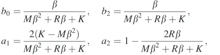
[image:7.612.51.295.641.712.2]b0¼ b
Mb2
þRbþK; b2 ¼
b
Mb2
þRbþK;
a1¼
2ðK&Mb2Þ
Mb2
þRbþK; a2 ¼1&
2Rb
Mb2
þRbþK;
(29)
wherebis the bilinear operator, which for a pre-warpedx0
is given by
b¼tan x0 ðx0T=2Þ
: (30)
In the PCS method one considers the quantity represented by the excitation signal spjn to describe the mechanical force
driving the sphere, that is, the discrete time equivalent of
F(t). Passing this signal through Hm(z) yields the sphere’s surface velocity!jn, which is then used in the final injection network.
In this formulation, the pulsating sphere is thought of as an external entity, unidirectionally coupled to the grid but not embedded into it, whose sole purpose is to generate a prescribed volume velocity. When this quantity is applied to a single grid node, the spatial period and nodal density of the rectilinear grid dictate that fluid emerges within a finite vol-ume ofV¼X3. Accordingly, by discretizing Eq.(13), a nu-merical equivalent ofq(x,t) is given by
qjni0¼q0
As
X3 !j
n
d½i&i0*: (31)
To derive the PCS injection filter and its corresponding coefficients g0 and g1, one needs to consider the type of scheme being used. Taking into account the additional scal-ing factors for the source term in Eq. (3), the coefficientg0
for a Yee-type scheme is given by
g0¼
z0kAs
X2 : (32)
Since in a Yee-scheme source differentiation is inherent in the update equations, the transfer function of the injection filter isHi(z)¼1. Considering the superposition constraint,
g1is set to unity in order to allow the update equation for air to operate over the source node. Accordingly, the final update equation for a Yee-type source node becomes
pjni0þ1¼ pjni0þ1
n o
þg0!jin0þ1¼ pjni0þ1
n o
þ ðc2TÞqjni0þ1; (33)
which is equivalent to the formulation proposed by Matheson.39 To develop the injection filter for the wave equation method, the physical definition of w(x, t) is fol-lowed. In the numerical domain, the differentiation con-straint described by Eq. (14), is adhered to by employing central finite differences approximating the time derivative ofq(x,t). Accordingly, the transfer function of the injection filter for the wave equation is
HiðzÞ ¼
1 2Tðz&z
&1
Þ: (34)
Considering the scaling constraints drawn from the formula-tion of qjni0, the coefficient g0for a wave equation source is given by
g0¼k
2q 0As
X : (35)
Adhering to the superposition constraint, g1 is set to unity, and the final update equation for a wave equation source node becomes
pjni0þ1¼ pjni0þ1
n o
þ2gT0ð!jin0&1&!jni0&1Þ
¼ pjni0þ1
n o
þc
2T
2 ðqj
nþ1
i0 &qjni0&1Þ: (36)
B. Generalizing source models
The signal processing chain described in this section can be used to generalize the process of modeling sources for FDTD simulation, where all existing source models, as well as the PCS, can be seen as special cases of the cascaded-filters method. To summarize this, TableIshows the differ-ent transfer functions and coefficidiffer-ents which may be used in the filter network in order to model different sources. For hard and soft sources the grid source function simply equals the excitation signal at the source position, that issgjni0 ¼spjn
with the only difference being the value ofg1which controls the superposition constraint. Within our formulation, in a Yee-type scheme the dimension of a hard source is pressure and the dimension of a soft source is velocity (due to the in-herent differentiation), whereas in wave equation schemes both sources have the dimension of pressure. Differentiated soft sources calculate the signal’s time derivative in the injection filter and therefore the injected quantity is volume velocity, however, their associated scaling coefficient g0 is appropriate for 1D grids. Transparent sources feature a proc-essing chain similar to that of soft sources, with the injection filter designed to compensate for the grid IR and, in Yee-schemes also reverse the effects of inherent differentia-tion. For the PCS method, the dimension ofspjnis
[image:8.612.70.288.44.99.2]mechani-cal force and, after the complete signal processing chain, the source function represents source density (in Yee methods), i.e., qjni0 ¼sgjni0, or its first time derivative (in wave equation methods), i.e.,wjni0 ¼sgjni0.
TABLE I. Generalization of source models using the cascaded filters approach. Inactive gains or filter blocks are indicated with a unity multiplier.
Hm(z) g0 Hi(z) g1
HS 1 1 1 0
SS 1 1 1 1
DSS 1 1
2Asq0cX z&z&
1
1
TS 1 1 1&I(z) 1
PCS (Yee) Eq.(28) 1
X2z0kAs 1 1
PCS (wave) Eq.(28) 1
Xk
2q
Readers who wish to make practical use of the unified source representation described in this section may down-load a dedicated Matlab function library, the Source
Modeling Toolbox,which has been made available online.40
V. RESULTS AND DISCUSSION
A. Prescribed pressure
To exemplify how the PCS can be designed to achieve a prescribed pressure field, a receiver was placed at the center of a 6-6-6 m domain, which was solved using the stand-ard rectilinear scheme (a¼0 andb¼0) at a sample rate of 16 kHz. A PCS was placed at a radial distance ofr¼1.5 m and an azimuth of 45.on the same plane as the receiver. The simulation was executed long enough for the entire signal to propagate from the source to the receiver but without intro-ducing any reflections from the boundaries. The excitation signal was designed with the impulse response of a MF FIR (M¼16 andfc¼0.075fs), which corresponds to the 2% dis-persion criterion for the standard rectilinear scheme.5 The magnitude of excitation was chosen such that the peak am-plitude of the filter’s output is normalized to a driving force of 250lN.
The mechanical filter of the PCS is characterized by the system resonance x0 and quality factor Q. In an optimal transducer design process, the designer would specify the desired values for these parameters and the remaining electro-mechanical quantities would be engineered accord-ingly. In this experiment, the radius of the pulsating sphere was arbitrarily chosen to be a0¼5 cm, and its mechanical constants corresponded to values of M¼25 g, f0¼100 Hz and Q¼0.7. It is worthwhile noting that a transducer of such small surface area would, in reality, produce a poor vol-ume velocity at low frequencies. However, while the nvol-umer- numer-ical model is governed by physnumer-ical laws, it is not bound by real world engineering constraints, and as such, it is possible
to design a small sphere of such low resonance.
Accordingly, the remaining damping and stiffness coeffi-cients are calculated from R¼x0M/Q and K¼Mx2
0,
respectively. As reference, a closed-form solution for Eq.(6) in free field is used. With a point-source approximation, the sound pressure at the distancer¼jjx&x0jjis given by28
pðr;tÞ ¼ q0
4pr d dtQ t&
r c
& '
: (37)
Numerical results were obtained using both the wave equa-tion method and the Yee-type method, and a reference response was calculated by passing the PCS volume velocity through Eq.(37). As shown in Fig.3(a), when using the PCS model, both methods are in agreement with the closed form solution.
B. Frequency response comparison
To study the pressure spectrum resulting from a PCS ex-citation, the same experiment was conducted using an inter-polated wideband scheme (a¼1/4 and b¼1/16), allowing for the high cutoff frequency to be increased to 0.25fs. The
PCS resonance was kept at f0¼100 Hz, which corresponds to 0.0063fs. This simulation was repeated for different values of Qranging from 0.5 to 2.0. As seen in Fig.3(b), the PCS model facilitates a means to design sources having a flat bandwidth between the system’s resonance and the cutoff frequency of the pulse-shaping filter. As expected from a second order linear system, adjusting Q controls the trade-off between the steepness of the low-frequency transi-tion band and the magnitude of resonance.
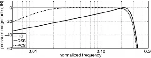
[image:9.612.316.560.46.144.2]For comparison of with other source models, three simu-lations were executed using an interpolated-wideband scheme, with a HS (also representative of the frequency response of a TS and a wave equation SS), a DSS (also rep-resentative of a Yee-type SS) and a PCS. All simulations used a MF FIR pulse with fc¼0.25fs, and the PCS was designed with a low resonance at f0¼0.167fs andQ¼0.7. For visual clarity, simulation outputs were normalized such that the peak value of each resulting impulse response is unity. As seen in Fig.4, the SS suffers from a severe roll off at low frequencies, which is to be expected due to differen-tiation (be it inherited in the source formulation or in the grid update equations in the case of a Yee method). Given that in the standard SS formulation, no mechanical or pulse shaping filter is explicitly defined, either the flatness require-ment is not met (if the signal is differentiated) or solution growth is not prevented (if it is undifferentiated). In the PCS model, the mass reactance of the sphere acts as an integrator which, in a physical manner, counters the effects of differen-tiation. Below its resonant frequency, the system is stiffness controlled, and as such, naturally acts as a DC-blocking fil-ter. The result is a source having a near-flat pressure
FIG. 3. Sound pressure at the receiving position of a domain excited using the PCS method. (a) Time domain comparison: Yee and wave equation (WE) methods plotted against the closed-form solution (CF). (b) Frequency spectra: wave equation method solved with different values ofQ.
FIG. 4. Calculated frequency response for three different source models,
HS&hard source (response similar to TS), DSS&differentiated soft source
(response similar to SS in Yee methods), PCS&physically constrained source. Excitation signals are MF FIR pulses ofN¼16 andfc¼0.25fs. PCS
[image:9.612.316.557.600.693.2]spectrum whose physical properties can be freely chosen by adjustingQandx0. In comparison to a HS, the spectrum of the PCS is flat abovef0but not down to DC; however, such a low-frequency response is essential for the exclusion of a DC component.
C. Numerical consistency
When simulating a physical system, changing numerical parameters should only affect the accuracy of the model. Accordingly, changing the sample rate of an FDTD model should not affect the magnitude of the generated sound field, a notion which is related to the scaling constraint discussed in
Sec. III. To test this, the wave equation FDTD method was
used with three sources, namely HS, DSS, and PCS. Transparent sources and undifferentiated soft sources have the same scaling coefficients as HS, thus as far as the magnitude of the soundfield is concerned, results can be appropriately deduced from the HS example. The simulation was repeated for three sample rates, namely 8 kHz (X¼74.37 mm), 12 kHz (X¼49.58 mm), and 18 kHz (X¼33.05 mm). An MF-FIR pulse-shaping filter withM¼16 andfc¼600 Hz was used in all simulations (regardless of the sample rate), thus ensuring that anomalies do not occur due to differences in the excita-tion signals.
It can be seen in Fig.5that the PCS is the only source model which results in a response whose magnitude is inde-pendent of sample rate. Nevertheless, in a one-dimensional problem, one would expect similar consistency for the case of a differentiated soft source, when it is appropriately scaled as described by Karjalainen and Erkut.14
D. DC and low-frequency artifacts
The theoretical analysis in Sec.III Dindicates that when soft sources in wave equation schemes include a DC compo-nent, a growing solution could occur. The concern arises when one uses an arbitrary SS, such as described by Eq. (19), where the source function directly equals the excitation
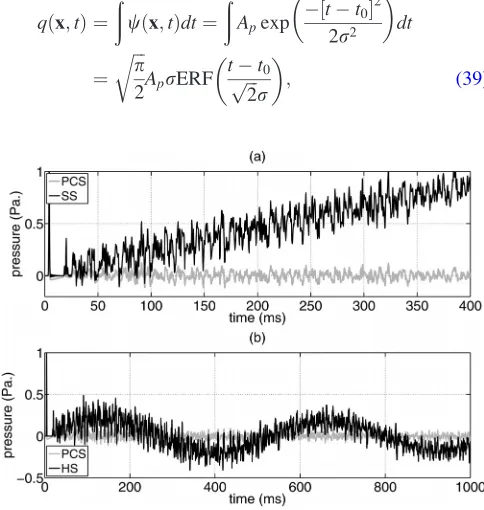
signal, and as such, may contain energy around DC. To test this, let us consider an arbitrary SS and a PCS, both of which are designed using a Gaussian pulse shaping filter. This pulse is unipolar and hence features a strong DC component. A re-ceiver was placed at the center of a 216 m3room at a dis-tance of 0.5 m from the source. The room was designed with uniform frequency independent boundaries, corresponding to a normal-incidence reflection coefficient of ^r¼0.997. Results from these simulations are displayed in Fig.6(a). For visual clarity, responses are normalized such that the direct component in the resulting responses equal 1 Pa. It is evident that the PCS response remains around the horizontal axis over time, whereas the soft source solution is linearly grow-ing. This growth is attributed to the accumulation of DC in the soundfield, and is unrelated to stability issues which nor-mally cause an exponential growth.
Such a growth is also sensible from a physical perspec-tive as a DC component insgjnindicates thatq(t) is not of fi-nite length, meaning that the equivalent excitation signal does not adhere to a time-compactness constraint. To explain this, it is useful to discuss the physical meaning of using the Gaussian as a source function in an undifferentiated SS model. Since such a source does not adhere to the differen-tiation constraint nor to any other mechanical constraints, then the excitation signal and source function are a direct nu-merical representation ofw(x,t),
sgjn ¼spjn'wðx;tÞjt¼nT: (38)
Since w(x, t) is defined as the first time derivative of
q(x,t), then following Eq.(14), the rate of fluid emergence due to the soft source is obtained by taking the integral of a Gaussian function, which yields
qðx;tÞ ¼
ð
wðx;tÞdt¼
ð
Apexp &½
t&t0*2
2r2
& '
dt
¼ ffiffiffi
p
2 r
AprERF
t&t0
ffiffiffi 2 p
r
& '
[image:10.612.316.558.448.703.2]; (39)
[image:10.612.54.297.525.710.2]FIG. 5. Pressure at the receiving position of a grid excited by (a) hard-source, (b) differentiated soft-hard-source, and (c) physically constrained hard-source, at three different sample rates.
FIG. 6. Sound pressure at the receiving position for a grid excited by a physi-cally constrained source (PCS) compared to (a) SS&undifferentiated soft source and, (b) HS&hard source. All source models employ a Gaussian pulse shaping filter (r¼31
3-10
-4
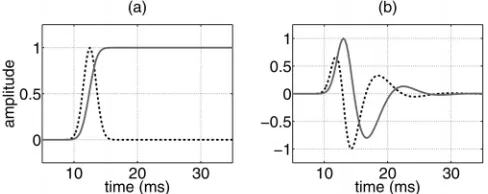
where ERF(%) is the Gauss error function,ris the pulse var-iance,Apis the amplitude of the pulse andt0denotes an ini-tial time shift. Figure 7 depicts w(t) and q(t), for such an undifferentiated soft source and for a physically constrained source.
When the PCS mechanical filter is damped (i.e.,a>0) and driven by an appropriately time-limited force, then both
q(t) and w(t) start at and decay to zero, indicating a finite source. However, this is not the case for the arbitrary SS. The fact that the grid signal represented by w(t) is time-limited can be misleading as, in physical terms, it only means that the source generating mechanism does not accel-erate before or after the excitation period. This does not mean that the source is not active. In fact, it can be seen for the SS that when w(t) decays,q(t) rises and stays at a con-stant value through the remaining simulation period, which indicates that even when w(t) is time limited, the source mechanism may still generate volume velocity. As one would expect,q(t) remains at a constant positive value which is equivalent to the generation of DC flow, meaning that the soundfield continuously gets pressurized by the source.
For the case of a HS injection, solution growth is not expected even if the excitation signal contains a DC compo-nent. This is because hard sources do not adhere to the super-position constraint, and as such, the existing pressure at the source node gets replaced by (rather than added to) the source function. As was identified by Jeong and Lam,21this prevents air particles at the source position from being able to perform rarefaction, which leads to a spurious low-frequency component in the resulting response. Figure6(b) compares the results of exciting the grid with a PCS and HS, both of which are based on a Gaussian excitation signal. It can be seen that while the HS solution does not display growth, it does contain a spurious low-frequency component (with a period of 582 ms).
E. Time limiting
Based on the assumption that excitation signals are rela-tively compact in time, it was further suggested by Jeong and Lam21that the HS scattering and low-frequency artifacts can be overcome by using sine-modulated pulses together with time-limiting the source injection process. To accomplish this, the source node is updated with a HS formulation until the associated excitation signal has decayed to zero, after which the regular update equations for the medium are used. This
workaround may appear useful for generating a soundfield similar to that of a transparent source, however it bears a cou-ple of complications. First, even if the excitation signal has decayed to zero, one cannot generally assume that the nodes surrounding the source are also null (although if the excitation signal is short and the source is sufficiently distant from a boundary, they might be). Additionally, it was shown in Fig. 7that in wave equation methods it is possible that even when the source function has decayed, the source is still physically active. Since the update equations for the medium involve temporal as well as spatial differentiation, any sudden change in the equations for the source node might introduce errors arising from the associated discontinuities.
VI. CONCLUDING REMARKS
A coherent approach to modeling sources in acoustic FDTD simulation has been made possible by representing the signal injection path with a chain of digital filters, and deriving the associated parameters from the physics and the numerics of the problem. The results presented in Sec. V show that a simple numerical monopole source can be for-mulated which is consistent with its continuous-domain counterpart, does not scatter wave energy, and affects a free-field pressure wave that is spectrally flat between specified cutoff frequencies. As such, the proposed physically con-strained source model offers an improved approach for meet-ing the aims and constraints inherent to FDTD excitation.
One principal limitation remains, in that the design of the source signal cannot escape the Gabor limit, meaning that there is inevitably some limit on the simultaneous time-frequency resolution one may achieve. Within this funda-mental restriction, the proposed method offers some design freedom through control of the resonance frequency and quality factor of the modeled pulsating sphere, both of which are intuitive design parameters from a physical as well as a spectral analysis perspective. As explained in relation to the simulation results presented in Secs.V AandV B, the value of the third design parameter, namely, the higher cutoff fre-quency, has to be chosen in relation to the numerical disper-sion properties of the employed scheme.
Since direct extension to multipole, plane-wave, and fur-ther spatially distributed excitation forms41is straightforward, the simple monopole model, as formulated in the present study, is directly applicable in FDTD grid excitation for a wide variety of acoustic applications. Among more elaborate future extensions, the formulation of bi-directional coupling between the source and the medium is of interest, in particular with regard to the study of room-loudspeaker interactions.
ACKNOWLEDGMENTS
The authors would like to thank Mark Avis for insightful discussions on electro-acoustic sound generation, and Jonathan Hargreaves for his helpful comments on the manuscript.
1
[image:11.612.53.297.604.701.2]J. G. Tolan and J. B. Schneider, “Locally conformal method for acoustic finite-difference time-domain modeling of rigid surfaces,” J. Acoust. Soc. Am.114, 2575–2581 (2003).
2
K. Kowalczyk and M. van Walstijn, “Modeling frequency-dependent boundaries as digital impedance filters in FDTD and K-DWM room acous-tics simulations,” J. Audio Eng. Soc.56, 569–583 (2008).
3
J. H€aggblad and B. Engquist, “Consistent modeling of boundaries in acoustic finite-difference time-domain simulations,” J. Acoust. Soc. Am.
132, 1303–1310 (2012).
4S. Bilbao, “Modeling of complex geometries and boundary conditions in
finite difference/finite volume time domain room acoustics simulation,” IEEE Trans. Audio, Speech, Lang. Process.21, 1524–1533 (2013).
5K. Kowalczyk and M. van Walstijn, “Room acoustics simulation using
3-D compact explicit F3-DT3-D schemes,” IEEE Trans. Audio, Speech, Lang. Process.19, 34–46 (2011).
6S. Bilbao, “Optimized FDTD schemes for 3D acoustic wave propagation,”
IEEE Trans. Audio, Speech, Lang. Process.20, 1658–1663 (2012).
7L. Savioja, “Real-time 3D finite-difference time-domain simulation of
low- and midfrequency room acoustics,” in 13th Int. Conf on Digital Audio Effects(2010).
8J. Sheaffer and B. Fazenda, “FDTD/K-DWM simulation of 3D room
acoustics on general purpose graphics hardware,” inProc. of the Institute of Acoustics(2010), Vol. 32.
9
C. Webb and S. Bilbao, “Computing room acoustics with CUDA - 3D FDTD schemes with boundary losses and viscosity,” inProc. IEEE Int. Conf. on Acoustics, Speech and Sig. Proc., Prague (2011).
10
K. Yee, “Numerical solution of initial boundary value problems involving Maxwell’s equations in isotropic media,” IEEE Trans. Antennas Propag.
14, 302–307 (1966).
11A. Taflove and S. Hagness,
Computational Electrodynamics (Artech
House, Boston, MA, 2000), pp. 175–224.
12S. Gedney,
Introduction to the Finite-difference Time-domain (FDTD) Method for Electromagnetics(Morgan & Claypool Publishers, San Rafael, CA, 2011), pp. 75–99.
13
D. Botteldooren, “Finite-difference time-domain simulation of low-frequency room acoustic problems,” J. Acoust. Soc. Am.98, 3302–3308 (1995).
14M. Karjalainen and C. Erkut, “Digital waveguides versus finite difference
structures: Equivalence and mixed modeling,” EURASIP J. Appl. Signal Process.2004, 978–989 (2004).
15H. Hacihabiboglu, B. Gunel, and A. Kondoz, “Time-domain simulation of
directive sources in 3-D digital waveguide mesh-based acoustical mod-els,” IEEE Trans. Audio, Speech, Lang. Process.16, 934–946 (2008).
16
T. Lokki, A. Southern, S. Siltanen, and L. Savioja, “Acoustics of epidau-rus studies with room acoustics modelling methods,” Acta Acust. Acust.
99, 40–47 (2013).
17D. Buechler, D. Roper, C. Durney, and D. Christensen, “Modeling sources in
the FDTD formulation and their use in quantifying source and boundary con-dition errors,” IEEE Trans. Microwave Theory Tech.43, 810–814 (1995).
18J. Schneider, C. Wagner, and O. Ramahi, “Implementation of transparent
sources in FDTD simulations,” IEEE Trans. Antennas Propag. 46, 1159–1168 (1998).
19
J. Schneider, C. Wagner, and S. Broschat, “Implementation of transparent sources embedded in acoustic finite-difference time-domain grids,” J. Acoust. Soc. Am.103, 136–142 (1998).
20
J. Redondo, R. Pic"o, B. Roig, and M. Avis, “Time domain simulation of sound diffusers using finite-difference schemes,” Acta Acust. Acust.93, 611–622 (2007).
21
H. Jeong and Y. Lam, “Source implementation to eliminate low-frequency artifacts in finite difference time domain room acoustic simulation,” J. Acoust. Soc. Am.131, 258–268 (2012).
22
P. Morse and K. Ingard,Theoretical Acoustics(McGraw-Hill, New York, 1986), p. 241.
23J. Strikwerda,
Finite Difference Schemes and Partial Differential Equations(SIAM, Philadelphia, PA, 2004), p. 34.
24
J. Botts and L. Savioja, “Integrating finite difference schemes for scalar and vector wave equations,” inIEEE Int. Conf. Acoust., Speech, Signal Processing(2013).
25M. R. Schroeder, “Integrated-impulse method measuring sound decay
without using impulses,” J. Acoust. Soc. Am.66, 497–500 (1979).
26S. M€uller and P. Massarani, “Transfer-function measurement with
sweeps,” J. Audio Eng. Soc.49, 443–471 (2001).
27R. San Mart
"ın and M. Arana, “Uncertainties caused by source directivity in room-acoustic investigations,” J. Acoust. Soc. Am.123, EL133–EL138 (2008).
28P. Morse and K. Ingard,
Theoretical Acoustics(McGraw-Hill, New York, 1986), p. 310.
29
A. Southern, D. Murphy, T. Lokki, and L. Savioja, “The perceptual effects of dispersion error on room acoustic model auralization,” inProc. Forum Acusticum, Aalborg, Denmark (2011), pp. 1553–1558.
30J. Botts, A. Bockman, and N. Xiang, “On the selection and
implementa-tion of sources for finite-difference methods,” in Proceedings of 20th International Congress on Acoustics(2010).
31T. Su, W. Yu, and R. Mittra, “A new look at FDTD excitation sources”
Microwave Opt. Technol. Lett.45, 203–207 (2005).
32
N. Ricker, “Wavelet contraction, wavelet expansion, and the control of seismic resolution,” Geophysics18, 769–792 (1953).
33X. Yuan, D. Borup, J. Wiskin, M. Berggren, and S. Johnson, “Simulation
of acoustic wave propagation in dispersive media with relaxation losses by using FDTD method with PML absorbing boundary condition,” IEEE Trans. Ultrason., Ferroelectr. Freq. Control46, 14–23 (1999).
34D. K. Wilson, S. L. Collier, V. E. Ostashev, D. F. Aldridge, N. P. Symons,
and D. Marlin, “Time-domain modeling of the acoustic impedance of po-rous surfaces,” Acta Acust. Acust.92(6), 965–975 (2006).
35O. Herrmann, “On the approximation problem in nonrecursive digital filter
design,” IEEE Trans. Circuit Theory18, 411–413 (1971).
36I. Khan and R. Ohba, “Explicit formulas for coefficients of maximally
flat FIR low/highpass digital filters,” Electron. Lett. 36, 1918–1919 (2000).
37J. Smith,
Introduction to Digital Filters: with Audio Applications(W3K Publishing, Stanford, CA, 2008), p. 272.
38
P. Morse and K. Ingard,Theoretical Acoustics(McGraw-Hill, New York, 1986), p. 315.
39R. J. Matheson, “Multichannel low frequency room simulation with
prop-erly modeled source terms-multiple equalization comparison,” in Audio Engineering Society Convention(2008), p. 125.
40
J. Sheaffer and M. van Walstijn, “Source modelling toolbox: WWW docu-ment and computer code,” http://code.soundsoftware.ac.uk/projects/smt/ (Last viewed October 2013).
41