Insights Gained by Visualization of a Wireless Channel Output using Self-Organizing Maps

(1)

International Journal of Emerging Technology and Advanced Engineering

Website: www.ijetae.com (ISSN 2250-2459,ISO 9001:2008 Certified Journal, Volume 4, Issue 11, November 2014)

462

Insights Gained by Visualization of a Wireless Channel Output

using Self-Organizing Maps

E. O. Otieno

1

, P. K. Kihato

2

, D. O. Konditi

3

1_{Electrical Engineering Program, Pan African University Institute for Basic Sciences, Technology and Innovation,}

P. O. Box 62000-00200, Nairobi, Kenya

2_{Electrical and Electronics Engineering Department, Jomo Kenyatta University of Agriculture and Technology,} P. O. Box 62000-00200, Nairobi, Kenya

3_{Department of Electrical and Communication Engineering, Multimedia University of Kenya, P. O. Box 15653-00503, Nairobi,}

Kenya

Abstract—The self-organizing map is an algorithm which can be used to establish the presence of various categories in a given numerical and non-numerical data and to visualize the complex topographical relations between the various such categories in a low dimensional and easily comprehensible display. In this paper, SOM has been used to visualize the output of a wireless channel in the presence of inter-symbol interference. An analysis of the symbol classification errors of the channel based on the constructed SOM has also been performed. A visualization of how the classification of channel outputs corresponding to various constellation points in a 16-QAM constellation is influenced by the value of their in-phase and quadrature components is presented. It is found that classification of various channel outputs is influenced to varying degrees by the value of their in-phase and quadrature components.

Keywords—Classification, Components, QAM, Self-Organizing Maps, Wireless Channel

I. INTRODUCTION

The self-organizing map hereafter referred to as SOM is a sheet like artificial neural network whose cells become specifically tuned to various input signal patterns or classes of patterns through an unsupervised learning process [1]. SOM preserves the topological relationships of the input training vectors so that input vectors which are close to each other are mapped on neighboring regions of the self-organized map. The SOM can be used for clustering as the cells of the map organize themselves according to the various categories present in the input data. A related application is classification as the fully formed map is used to classify a candidate input. For an even more insightful analysis, each component of the map weight vectors (corresponding elements of the weight vectors of all map nodes) may be displayed in a gray-scale to illustrate the values of the components [2].

Some of the applications of SOM in telecommunications have been described in [3]-[8].In this paper, SOM is used to study the effects of the channel on a digitally modulated input. We visualize how the wireless channel output looks like in the presence of severe inter-symbol interference. Here we visualize the distribution of the various classes of input in the channel output vector space and the topological relationship of the input digital modulation constellation and the interfering channel output. A SOM developed from channel output is used to categorize the channel output and an error analysis is performed on the misclassified symbols. We then draw a component map illustrating the values of corresponding elements of SOM weight vectors in gray-scale. An illuminating view of how the classification of various classes of channel input is dependent on their in-phase and quadrature components results.

The rest of this paper is organized as follows. In section 2 we briefly describe the Kohonen Self-Organizing Map. The description contained herein has been derived mainly from [1] and [9].Next we describe the procedure by which the SOM was trained. Then we present the results of an error analysis performed from the misclassification of the SOM. We then present the component planes of the map and draw conclusions from them.

A. The Self-Organizing Map Algorithm

a)The number of cells or nodes of the SOM is selected. The recommended number is about

samples training

of number



10

(2)

International Journal of Emerging Technology and Advanced Engineering

463 The method of initialization can be random where each

node weight vector is initialized using random values which lie within a certain range.

c)For the required number of steps, an input vector is picked at random from the training samples and presented to the network. If the training samples are fewer than the required number of steps, then they are recycled until the required number of steps is attained. As a vector is picked at random and presented to the network, every node in the network is examined to calculate whose weights are closest to the input vector. The winning node is called the best matching unit

(BMU). Let

x





n be an input data vector and

]

,

[

_i₁ _i₂

i

m



be the weight vector of a cell

i

. Then

the smallest of the Euclidean distances

x



m

_i is

selected to be the BMU signified by the postscript

c

.

i

x

m

c



argmin



d)The BMU and the nodes that are close to the BMU up to a certain distance (neighbourhood radius) will activate each other to learn from the input vector. For this purpose a neighbourhood radius is calculated which starts large and reduces at each time step. A function commonly used to calculate the neighbourhood of the winning neuron is

)

(

2 exp(

).

(

)

(

₂ 2

t

r

t

h

_ci c i









Where



(

t

)

is a scalar valued learning rate and



(

t

)

is the width of the kernel. Both



(

t

)

and



(

t

)

are monotonically decreasing functions of time.

e)Nodes that are within the radius of the BMU are updated according to the equation below

)]

(

)

(

)[

(

)

(

)

1 (

t

m

t

h

t

x

t

m

t

m

_i





_i



_ci



_i

f) The algorithm is repeated from step c) for the required number of steps

The training is usually split in two phases. In the first phase, the learning rate starts from a large value and reduces to a small value. At the same time, the radius of the neighborhood reduces from an initial value of more than half the diameter to say one unit.

Then in the second phase of training, the neighborhood is confined to a small area close to the BMU if not only the BMU. In this phase the small learning rate is maintained over a long period. The first phase is the ordering phase when the node weights become properly ordered in the input vector space and the second phase is the fine-tuning phase [1].

Visualization of SOM provides more insight about the training data and its structure. An important visualization tool is the SOM component plane [10]. For each component of the SOM vectors there is a component plane representing the value of each neuron.

II. SIMULATIONS

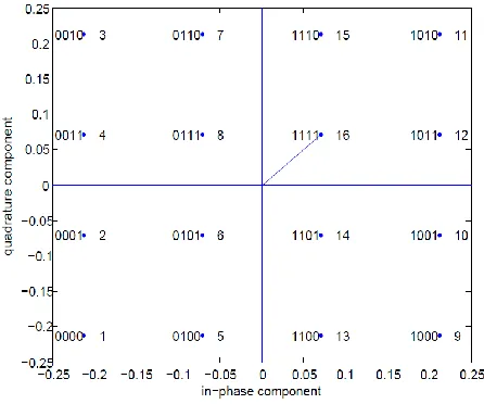
Un-modulated 16-QAM signals whose gray coded constellation is shown in Figure 1 below were generated.

The 16 signal constellation points have been shown with their gray codes to the left and the decimal equivalent to the right. Each constellation point will henceforth be referred to by their decimal equivalent. In clustering terminology we will refer to each of the constellation points as a class, so that there are 16 classes for the drawn constellation and each class is referred to by its decimal equivalent. Note that the energy of a specified constellation point is given by the length of the vector originating from the origin (point (0, 0)) to the specified point. For example, the energy of constellation point 16 is given by the length of the drawn vector. The average constellation energy is given by the sum of the energy for all the constellation points divided by the number of constellation points.

In the second step, a value is randomly generated on the discrete uniform distribution in the range 1-16, and then the constellation point with the decimal equivalent to this value is sent over the symbol interval. For the experiments in this paper, about 1000 such symbols are sent over a wireless channel.

(3)

International Journal of Emerging Technology and Advanced Engineering

[image:3.612.54.277.187.373.2]

464 For training the SOM, we used the SOM_PAK program package which contains all programs necessary for the correct application of the self organizing map algorithm in the visualization of complex experimental data [2].

Figure 1: 16-QAM constellation used for the experiment

A map was created of 160 units arranged in a rectangular topology with 16 units in the x-direction and 10 units in the y-direction. Random initialization of the map was used. The training of SOM was carried out in two phases. In the first phase the parameter used were: 30,000 steps, initial learning rate parameter was 0.05 and initial radius of the training area of SOM was set to 8 units. In the second phase the parameters used were: 70,000 steps, initial learning rate parameter is 0.02 and the initial radius of the training area of SOM is 2 units.1000 maps were created using the parameters and the best one was picked as the one which gives the lowest average quantization error. The quantization error is the Euclidian distance between a reference vector of the trained map and the input vector which most resembles it. The training samples are used for the purpose of computing the average quantization error.

III. RESULTS AND DISCUSSION

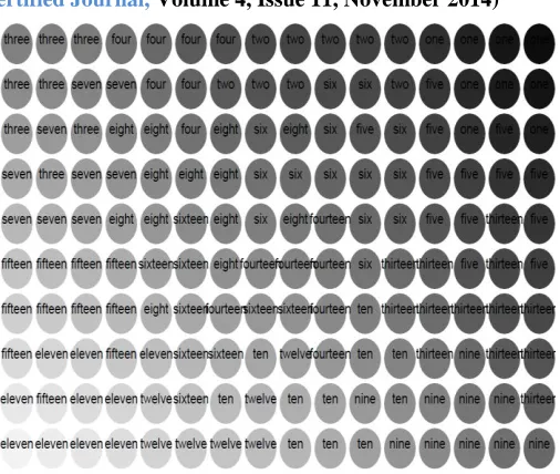
The trained map was calibrated using known labels of the classes of the various channel output. For example, a node in the trained map which mostly wins the representation of input vectors belonging to class 1 is labeled as ―one‖. The resultant map labels for the final map vectors are illustrated in Figure 2 where each map weight vector is plotted at the position of its components on a Cartesian plane and its marker is the numeric value of its class label.

[image:3.612.328.564.228.407.2]

Since the final map values reflect the density and topographical relationships in the training samples, we can thus make observations about the structure of the channel output based on the final map values. Comparing Figure 2 and channel input constellation in Figure 1, it is observed that the channel output is a rotated version of the channel input.

Figure 2: Plot of SOM final vector values and the class each vector represents

The fully trained SOM was used to classify the channel output. Of the 1000 symbols transmitted over the interfering channel, 70% were correctly classified. An error analysis was then done on the misclassified symbols to determine what each class of symbol is likely to be misclassified to. The results found indicate that a symbol is likely to be misclassified to the symbols whose gray codes differ from that of the current symbol by one bit. In other words, the validity of gray coding is verified.

The component planes of the first and second components of the map weight vectors are plotted using grayscale in Figure 3 and Figure 4 respectively.

(4)

International Journal of Emerging Technology and Advanced Engineering

465 Similarly, the second components of map weight vectors correspond to the quadrature component of channel input. In the same Figure 3 it is also seen that classes 3, 4 and 7 are weakly dependent on the real part of the channel output. The remaining classes are here taken to be moderately dependent on the first component.

[image:4.612.324.577.125.339.2]

From Figure 4, we see that classification of classes 1, 2, and 5 are least dependent on the second component of map weight vectors while classes 11, 12 and 15 are most strongly dependent on the second component. The rest of the classes are moderately dependent on the second component of the map weight vectors.

Figure 3: A component map for the first component of map weights. Note the lighter regions in the bottom right corner indicating classes

which depend strongly on the first components and the darkest regions in the top left corner indicating the classes on which the first

[image:4.612.48.290.278.476.2]

component has the least effect.

Figure 4: A component map for the second component of the final map weights.

(5)

International Journal of Emerging Technology and Advanced Engineering

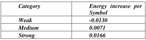
[image:5.612.44.292.175.244.2]

466 TABLE I

Average Increase in Energy per Symbol for the Symbols that are Weakly, Moderately and Strongly Influenced by the In-phase

Component.

Category Energy increase per

Symbol

Weak -0.0130

Medium 0.0071

Strong 0.0166

From the above discussion, it is seen that classes which are strongly influenced by a component of the map weight vectors have the most desirable response to a change in that component in the input symbols whereas classes which are least influenced by a component of the map weight vectors have the least desirable response to a change in that component in the input symbols.

IV. CONCLUSION

In this paper, Self Organizing Maps were used to gain some insights into the effects of a wireless channel on digitally modulated symbols sent over an interfering channel. The structure of channel output was visualized and it was found that the output resembles a rotated digital modulation constellation. A classification analysis was performed with the resulting SOM and the correctness of gray coding for the channel was verified. A component map for the first and second component of map weight vectors reveals that the different classes of channel output are influenced to varying levels by the in-phase and quadrature components. The authors are working on a paper to demonstrate how this result can be used to mitigate against inter-symbol interference in a wireless channel.

REFERENCES

[1] T. Kohonen, ―The Self-Org anizing Map,‖ in Proc. IEEE, Vol. 78, Sept. 1990, pp. 1466–1469.

[2] T. Kohonen, J. Hynninen, J. Kangas, and J. Laaksonen. ―SOM_PAK: The Self-Organizing Map Program Package.” Internet: http://www.isegi.unl.pt/ensino/docentes/fbacao/som_pak.pdf, April 7, 1995 [May 2, 2014].

[3] K. Raivio, ―Receiver Structures Based on Self-Organizing Maps,‖ Ph.D. Thesis, Helsinki University of Technology, Espoo, Finland, 1999.

[4] K. Raivio, J. Henriksson, and O. Simula, ―Neural detection of QAM modulation in the presence of interference,‖ In Proc. ICNN’95, IEEE International Conference on Neural Networks, Piscataway, NJ. IEEE Service Center, 1995b, vol. 4, pp. 1566-1569.

[5] K. Raivio, J. Henriksson, and O. Simula, ―Neural detection of QAM signal with strongly nonlinear receiver,‖ In Proc. of WSOM’97, Workshop on Self Organizing Maps, Espoo, Finland, June, 4-6, Helsinki University of Technology, Neural Networks Research Center, Espoo, Finland, 1997b, pp. 20-25.

[6] H. Lin, X. Wang, J. Lu, and T. Yahagi, ―Analysis of a neural detector based on self-organizing map in a 16-QAM system, ―IEICE Trans. on Communications,‖ E84-B9, pp. 2628-2634, 2001 [7] D. Watkins, ―Discovering geographical clusters in a U.S.

telecommunications company call detail records using Kohonen self organizing maps,‖ In PADD98. Proc. of the Second Int. Conf. on the Practical Application of Knowledge Discovery and Data Mining,‖ Practical Application Co. Ltd, Blackpool, UK, 1998, pp. 67-73. [8] K. Raivio, J. Henriksson, and O. Simula, ―Interference cancellation

for PAM modulation using neural networks,‖ In Proc. of the Finnish Signal Processing Symposium, 1995a, pp. 50-54.

[9] S. M. Guthikonda. ―Kohonen self-organizing maps‖ Internet: http://www.shy.am/wp-content/uploads/2009/01/kohonen-self-organizing-maps-shyam-guthikonda.pdf, Dec. 2005 [May 10, 2014]. [10] J. Vesanto, ―SOM-based data visualization methods,‖ In Intelligent

Data Analysis, Volume 3, Number 2, Elsevier Science, pp. 111-126, 1999.