Cost sensitive decision tree learning using a multi armed bandit framework

(1)

COST-SENSITIVE DECISION TREE LEARNING

USING A

MULTI-ARMED BANDIT FRAMEWORK

Susan Elaine LOMAX

SCHOOL OF COMPUTING, SCIENCE AND ENGINEERING,

INFORMATICS RESEARCH CENTRE, COLLEGE OF SCIENCE AND

TECHNOLOGY, UNIVERSITY OF SALFORD

(2)

i

TABLE OF FIGURES

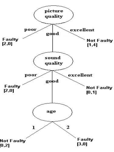
Figure 1 Decision tree after ID3 has been applied to the dataset in Table 1 ... 11

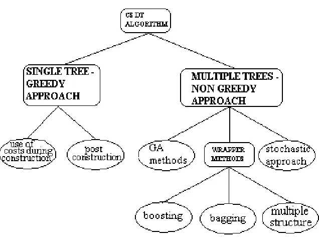
Figure 2 Taxonomy of Cost-Sensitive Decision Tree Induction Algorithms ... 19

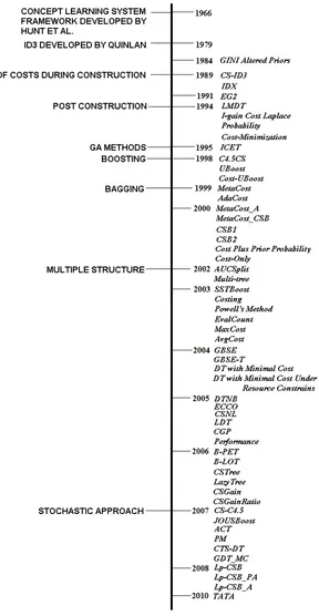
Figure 3 A timeline of algorithms ... 21

Figure 4 Decision tree after EG2 has been applied to the dataset in Table 1 ... 24

Figure 5 Decision tree when DT with MC has been applied to dataset in Table 1 ... 31

Figure 6 Linear Machine ... 34

Figure 7 Example ROC ... 38

Figure 8 Illustration of mapping ... 42

Figure 9 Multi-tree using the example dataset ... 59

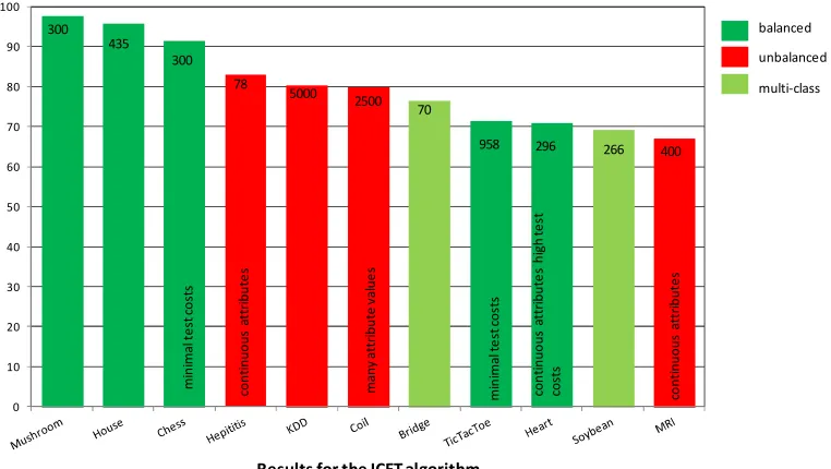
Figure 10 Using ICET’s results to demonstrate weaknesses of cost-sensitive decision tree algorithms ... 71

Figure 11 Illustration of the single pull and look-ahead bandit in the algorithm ... 77

Figure 12 Generate P bandits and calculate cost at the end of each path ... 79

Figure 13 Multi-Armed Cost-Sensitive Decision Tree Algorithm (MA_CSDT) ... 81

Figure 14 To calculate the number of potential unique bandit paths in a dataset ... 85

Figure 15 Results illustrating the fluctuating values obtained using artificial datasets ... 87

Figure 16 Desired tree chosen by a given strategy ... 88

Figure 17 Graphs showing do nothing costs versus cost obtained for each of the types of classes ... 105

Figure 18 Graphs showing multi-class datasets in their 3 groups of misclassification costs: mixed, low, high ... 107

Figure 19 Comparing mean values obtained with values obtained by a given strategy ... 111

Figure 20 Rules extracted using J48 accuracy-based algorithm on examples in the results analysis file ... 117

Figure 21 Heart dataset processed using pruned versions of the cost-sensitive algorithms and flare dataset using un-pruned versions of the cost-sensitive algorithms... 130

Figure 22 The krk dataset: top processed using pruned version; bottom processed using un-pruned version of cost-sensitive algorithms ... 133

(5)

iv

TABLE OF TABLES

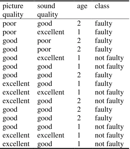
Table 1 Example dataset ‘Television Repair’ ... 10

Table 2 Pay-off matrix for Prisoner’s Dilemma ... 14

Table 3 Cost-sensitive decision tree induction algorithms categorized with respect to taxonomy by time ... 20

Table 4 Definitions of equations ... 22

Table 5 Example of a cost matrix of a four class problem ... 29

Table 6 Typical cost matrix for two-class problems ... 68

Table 7 Main characteristics of datasets used in the comparison ... 68

Table 8 Example of the multi-armed bandit algorithm choosing an attribute ... 80

Table 9 Values of P lever pulls for each dataset ... 96

Table 10 Details of each experiment, settings and frequency (%) of best and worst results from the analysis file ... 98

Table 11 Summary of dataset information including mean values obtained from the analysis file ... 100

Table 12 Manually obtained parameter settings based on description of a dataset and frequency of class 1 examples ... 114

Table 13 Accuracy rates obtained from J48 predicting classes from parameter settings ... 115

Table 14 Percent of trees not grown by dataset for the six algorithms in the evaluation with the cost matrices producing the least trees ... 124

Table 15 Percent that each cost-sensitive algorithm achieves the lowest cost or highest accuracy for a cost matrix for both pruned and un-pruned versions ... 126

Table 16 Summary of whether MA_CSDT has met its aims for each dataset ... 127

(6)

v

ACKNOWLEDGEMENTS

Thanks to John Bacon, Mathscope, University of Salford for help in the development of the solution to calculating potential unique bandit paths and to my co-supervisor Dr Chris Bryant for pointing me in the right direction. Thanks to Dr K J Abrams for her help in understanding the Annealing dataset along with advice regarding allocation of test costs and groupings of attributes. Thanks also to Duncan Botterill, without whose help the experimental results would have taken even longer to process.

The majority of my thanks go to my supervisor Professor Sunil Vadera for his continuing help and support whilst undertaking this research. He has given me the confidence to believe in myself when otherwise I would not.

As part of this research the following papers have been published which contain some of the content of this thesis:

An Empirical Comparison of Cost-Sensitive Decision Tree Induction Algorithms published in Expert Systems: The Journal of Knowledge Engineering, July, Vol. 28, No 3, 227 – 268. A Survey of Cost-Sensitive Decision Tree Induction Algorithms published in ACM Computing Surveys, Vol. 45, No. 2, Article 16.

A Multi-Armed Bandit Approach to Cost-Sensitive Decision Tree Learning published in Data Mining Workshops (ICDMW), 2012 IEEE 12th International Conference, 10-13 December 2012, Brussels, Belgium, 162 – 168.

(7)

vi

ABSTRACT

Decision tree learning is one of the main methods of learning from data. It has been applied to a variety of different domains over the past three decades. In the real world, accuracy is not enough; there are costs involved, those of obtaining the data and those when classification errors occur. A comprehensive survey of cost-sensitive decision tree learning has identified over 50 algorithms, developing a taxonomy in order to classify the algorithms by the way in which cost has been incorporated, and a recent comparison shows that many cost-sensitive algorithms can process balanced, two class datasets well, but produce lower accuracy rates in order to achieve lower costs when the dataset is less balanced or has multiple classes.

This thesis develops a new framework and algorithm concentrating on the view that cost-sensitive decision tree learning involves a trade-off between costs and accuracy. Decisions arising from these two viewpoints can often be incompatible resulting in the reduction of the accuracy rates.

(8)

vii methodology to explore potential attributes and exploit the attributes which maximizes the reward.

(9)

1

CHAPTER 1: INTRODUCTION

1.1 The motivation for the research in this thesis

Decision trees are a natural way of presenting a decision-making process, because they are simple and easy for anyone to understand (Quinlan 1986). Learning decision trees from data however is more complex, with most methods based on an algorithm known as ID3 which was developed by Quinlan (1979, 1983, 1986). ID3 takes a table of examples as input, where each example consists of a collection of attributes, together with an outcome (or class) and induces a decision tree, where each node is a test on an attribute, each branch is the outcome of that test and at the end are leaf nodes indicating the class to which an example, when following that path, belongs. ID3, and a number of its immediate descendents, such as C4.5 (Quinlan 1993), CART (Breiman et al. 1984) and OC1 (Murthy et al. 1994) focused on inducing decision trees that maximized accuracy.

However, several authors have recognized that in practice there are costs involved (e.g. Breimen et al. (1984); Turney (1995, 2000); Elkan (2001)). For example, it costs time and money for blood tests to be carried out (Quinlan et al. 1987). In addition, when examples are misclassified, they may incur varying costs of misclassification depending on whether they are false negatives (classifying a positive example as negative) or false positives (classifying a negative example as positive). This has led to many studies which develop algorithms that aim to induce cost-sensitive decision trees.

(10)

2 Lomax and Vadera (2011) have evaluated algorithms which have incorporated these costs into the construction using extensions to statistical measures, genetic algorithms, or boosting and bagging techniques. Experiments were carried out over a range of cost matrices and showed that using both costs in the construction was the better method. However, on a later examination of the results from the algorithm which performed better overall (ICET introduced by Turney (1995)), variations in performance revealed weaknesses where the algorithm produced poorer results than would be expected. Contributing factors to the variation in performances are thought to be large numbers of attributes, differing numbers of attribute values, class distribution, number of classes and differing costs. Trade-off between high misclassification costs result in the sacrifice of the accuracy rate. The nature of the dataset may account for some of the discrepancies. These could influence how easy it is for the algorithm to classify examples.

Although in the literature, it has always been suggested that Game Theory is different to decision theory (an idea utilized in some decision tree algorithms) and therefore caters to different decision situations, it has been suggested that it can be applied in a Machine Learning capacity (Cesa-Bianchi and Lugosi 2006) and could be used for prediction as both disciplines have in common the idea that past experience predicts future events.

(11)

3 Pay-off functions are assigned to the strategies in order to help make the decisions. Picking strategies which would maximize pay-off is the desired outcome with a trend towards simplicity. Finding the simplest assumption needed (Occam’s razor1) is the ideal outcome (Rasmusen 2001). Pay-offs are shown using a matrix and strategies can be illustrated using decision-tree like structures.

Use of costs within the decision tree learning process has introduced many interesting problems involving the trade-off required between accuracy and costs. It is clear that, whilst there are existing cost-sensitive decision tree algorithms which can solve two-class balanced problems well, other types of problems cause difficulties. In particular several authors have recognized that there can be a trade-off between accuracy and minimizing cost (Lomax and Vadera 2009, 2011) or a reduction in performance (Ting 2000a).

Hence, this research aims to utilize Game Theory as a basis for developing a cost-sensitive decision tree algorithm, which aims to be able to address the trade-off between accuracy and cost that has been observed in previous studies.

1.2 Research methodology

Different methodologies have been studied and the most appropriate one is selected for this PhD. The methodologies studied are grouped under three categories:

1

(12)

4

• Constructive Methods

These deal with conceptual and technical development and may not be as empirically based as other methods. They may involve evaluating prototype software against defined criteria or testing prototypes (Livari et al. 1998).

• Nomothetic Methods

These are positivism, where the idea is that the world exists externally and measurements should be through objective methods. It encourages statistics and experiments (Livari et al. 1998). Methods in this category are generally ‘laws’ i.e., laws of physics etc, and scientific methods such as hypothesis testing, mathematical analysis, experiments, field studies and surveys. They will be quantitative in the data collection and confirmatory.

• Idiographic Methods

These are interpretivism, which is the opposite of positivism. It encourages the appreciation of constructions and meanings which people have, not reporting facts, but dealing with the interpretations of them (Livari et al. 1998). Methods in this category are generally case studies and action research, dealing with direct experience. Case studies and action research deal in on-the-spot fact finding. The researcher learns about system requirements or how things work by visiting the place which requires it or has information about it. They are useful for studying how and why things happen. They are performed by interviews, observations, which are either overt or covert, and document analysis.

(13)

5 A method named GQM (Goal, Question, Metric) (Basili and Weiss 1984) is recommended to be used in the area of software development. GQM is a measurement mechanism used in order to obtain feedback and evaluation in software development. Its aim is to focus on specific goals and must be defined in a top-down fashion. It is ideally suited to this area as there are many observable characteristics such as lines of code, number of defects or complexity, making other methods which are metric-driven and bottom up unworkable (van Solingen et al. 2002). The GQM approach is to define goals, which are then refined into questions, and metrics are used in order to gain enough information so that the questions can be answered.

In this thesis, the goal is to develop a framework which uses the trade-off required between accuracy and costs in order to achieve low costs and high accuracy which is required in cost-sensitive learning. As a result of this goal, the following questions have been developed:

1. How well do existing cost-sensitive decision tree algorithms perform? 2. What are the weaknesses of existing cost-sensitive decision tree algorithms?

3. Is it possible to minimize costs and minimize the sacrifice of the accuracy rate which occurs in cost-sensitive decision tree learning?

4. Will using a technique, which has been developed to deal with trade-off by using pay-offs, help in achieving the aim of cost-sensitive decision tree learning?

(14)

6

1.3 Research hypothesis, aims and objectives

The Research Hypothesis put forward is that cost-sensitive decision tree learning involves a trade-off between decisions based on accuracy and decisions based on costs and that Game Theory can be utilized to develop an algorithm that improves upon the performance of existing algorithms. By using Game Theory, it may be possible to explore the opposing decisions in such a way as to decide that a compromise can indeed be reached. Any algorithm which aims to be a cost-sensitive one will need to achieve this trade-off in order to function correctly. The aim of this PhD is therefore to show what happens to accuracy and costs in the trade-off and to find a framework that can use the trade-off effectively to achieve the low costs and high accuracy required in cost-sensitive learning. In order to test this hypothesis the thesis objectives are:

1. To survey and review existing cost-sensitive decision tree algorithms in order to investigate ways in which costs have been introduced into the decision tree learning process and at which stages they have been introduced

2. To evaluate existing cost-sensitive decision tree algorithms in order to discover whether these algorithms are successful over many types of problems or are only effective for some types of problems, for example binary class datasets or balanced datasets

3. To develop a new cost-sensitive decision tree algorithm which is based on Game Theory

(15)

7

1.4 Outline of thesis

The rest of the thesis is structured as follows:

• Chapter 2: Background

This chapter presents the background to decision tree learning and Game Theory

• Chapter 3: Survey of existing cost-sensitive decision tree algorithms

This chapter presents the results of a literature search which identifies existing cost-sensitive decision tree algorithms and categorizes them into classes by the way the costs have been introduced

• Chapter 4: The development of a new multi-armed bandit framework for

cost-sensitive decision tree learning

This chapter presents an analysis of previous cost-sensitive decision tree algorithms, highlights their weaknesses and suggests a new framework using multi-armed bandits. Experiments are carried out in order to fine-tune the algorithm and an extension is also developed. The experimental methodology is also presented

• Chapter 5: Investigating parameter settings for MA_CSDT

This chapter presents an extensive investigation into four areas. These four areas address the parameter settings, in particular those which determine whether it is worthwhile to continue the induction process, determining the number of lever pulls to set for a dataset, which version and strategy is better and to investigate how different combinations of parameter settings and strategies can be used to obtain good results. Guidelines to setting these parameters are also discussed

• Chapter 6: An empirical comparison of the new algorithm with existing cost-sensitive

(16)

8 This chapter presents the results of the empirical comparison and evaluation against existing cost-sensitive decision tree algorithms and an accuracy-based algorithm in order to determine whether the aim of the algorithm can be met

• Chapter 7: Conclusions and future work

(17)

9

CHAPTER 2: BACKGROUND

2.1 Decision tree learning

Given a set of examples, early decision tree algorithms, such as ID3 and CART, utilize a greedy top-down procedure. An attribute is first selected as the root node using a statistical measure (Quinlan 1979, 1983; Breiman et al. 1984). The examples are then filtered into subsets according to values of the selected attribute. The same process is then applied recursively to each of the subsets until a stopping condition, such as all of the examples in the subset being of the same class. The leaf nodes are then assigned the majority class as the outcome. Researchers have experimented with different selection measures, such as the GINI index (Breiman et al. 1984), using chi-squared (Hart 1985) and which have been evaluated empirically (Mingers 1989). The selection measure utilized in ID3 is based on Information Theory which provides a measure of disorder, often referred to as the entropy, and which is used to define the expected entropy, E for an attribute A (Shannon 1948; Quinlan 1979; Winston 1993). The entropy of an attribute A is defined as:

() = ∑_∈(). ∑ – P(|)log2(P(|)))_∈ (2.1)

where a ∈ A are the values of attribute A, and the c ∈ C are the class values.

This formula measures the extent to which the data is homogeneous. For example, if all the data were to belong to the same class, the entropy would be '0'. Likewise if all the examples belonged to different classes, the entropy would be '1'. ID3 uses an extension of the entropy by calculating the gain in information (I) achieved by each of the attributes if they were

(18)

10

ID3: = () − () (2.2)

where E(D) = ∑_∈ – , calculated on the current training set before splitting.

Although Quinlan adopted this measure for ID3, he noticed that the measure is biased towards attributes which have more values, and hence proposed a normalization, known as the Gain Ratio, which is defined by:

C4.5: !"#$%" = &'

&()*' +ℎ-.- #/ = ∑ –

0

∈ 0

(2.3)

C4.5 was also developed to include the ability to process numerical data and deal with missing values. Figure 1 presents the tree that result from applying the ID3 procedure to the examples in Table 1. At each leaf is the class distribution, in the format of (faulty, not faulty).

picture

[image:18.595.195.403.468.707.2]

quality sound quality age class poor good 2 faulty poor excellent 1 faulty good poor 2 faulty good poor 2 faulty good excellent 1 not faulty good good 1 not faulty good good 2 faulty excellent good 1 faulty excellent excellent 1 not faulty excellent good 2 not faulty good good 2 faulty good good 2 faulty good good 1 not faulty excellent excellent 1 not faulty excellent good 1 not faulty

(19)

11 Once a decision tree has been built, some type of pruning is then usually carried out. Pruning is the term given to that of replacing one or more sub-trees with leaf nodes. There are three main reasons for pruning. One is that it helps to reduce the complexity of a decision tree, which would otherwise make it very difficult to understand (Quinlan 1987), resulting in a faster, possibly less costly classification. Another reason is to help prevent the problem of over-fitting the data.

Figure 1 Decision tree after ID3 has been applied to the dataset in Table 1

(20)

12

2.2 Game Theory

Game Theory is a discipline which deals in trade-off. It deals with types of decision making where there may be more than one decision-maker. Game Theory (Davis 1983; Osborne 2004) states that it is decision making with two decision-makers, which it denotes as ‘players’. At least two players choose a strategy (make a decision) and as a result a reward or pay-off occurs. Each player must worry about what the other is doing. Pseudo-players have actions taken in a mechanical way; Nature is an example of a Pseudo-player (Rasmusen 2001). Game Theory is the theory of many games not just one (Davis 1983).

Game Theory differs from other types of decision making problems because as decision-makers are manipulating the environment i.e. deciding how much advertising space to purchase, the environment i.e. other decision-makers are trying to do the same (Davis 1983). Game Theory has been used in disciplines such as economics, social science, political science and biology and applied to tasks such as price fixing, advertising, and strategies used in competitive business.

(21)

13 Decisions are linked to goals and the consequences of each option must be known in order to make the solution easy. The best strategy is chosen in order to reach the goal. If chance plays a role, decisions are harder to make (Davis 1983). Pay-off functions are assigned to strategies in order to help make the decisions. Picking strategies which maximizes pay-off is the desired outcome with a trend towards simplicity; finding the simplest assumption needed is the ideal outcome (Rasmusen 2001). Pay-offs are shown using a matrix and strategies can be illustrated using decision-tree like structures.

Models are not either right or wrong but useful or not depending on the purpose for which they are used. The models are examined in order to analyze their implications, to either confirm an idea or suggest it is wrong. This analysis should help understand why it is wrong. Time is absent from the model. Each player chooses their actions “simultaneously” in that no player is informed when an action is chosen or what action another player has chosen (Osborne 2004). The assumption is that actions are chosen once and for all. It is assumed that all players will try to do their best. A Nash Equilibrium is a pair of strategies which, when applied, results in both players choosing the same option as neither wishes a change in strategy. It occurs when all players make the best reply to the strategy choice of the others (Nash 1950a, 1950b). For example if a player knew that the other player would always choose a particular strategy, they could maximize their pay-off by choosing the same strategy.

There are three main categories of games in Game Theory. These are (i) the two-person zero-sum game (ii) the two-person non-zero-zero-sum game and (iii) the n-person game first defined by

(22)

14 the case. An example of a zero-sum game would be Matching Pennies where each player has two strategies; heads or tails. The Prisoner’s Dilemma is an example of a non-zero-sum person game.

The Prisoner’s Dilemma Game is one of the most well known ‘games’ in Game Theory (Binmore 2007). Two suspects have been arrested for a minor crime, for instance handling stolen goods, for which there is ample evidence. However, they are suspected by the police of the greater crime of burglary for which there is only circumstantial evidence and no proof. The suspects are both offered the same deal:

• If one confesses and turns Queen’s evidence, and the other does not, he will go free and the other goes to jail for a maximum prison term.

• If both suspects confess they both go to jail for a minimum prison term for burglary.

• If both suspects remain silent they both go to jail for a year for the handling charge as

there is no evidence for any other wrong-doing.

The assumption is that each prisoner will try their upmost to do what is best for themselves. The pay-offs are displayed in a matrix presented in Table 2.

suspect 2

confess do not confess

suspect1 confess min, min 0, max

do not confess max, 0 1,1

(23)

15 Each player has two basic choices; they can act co-operatively or un-cooperatively. For any fixed strategy of the other players, a player always does better by playing un-cooperatively than by playing co-operatively (Binmore 2007).

Another well-known game is the Hawk-Dove Game, where two birds, for example pheasants, may contest a resource such as food. The two birds can either act passively or aggressively in this kind of situation (Binmore 2007). A passive bird would surrender the food to an aggressive bird. Two passive birds would share the food but two aggressive birds would fight. Passive birds are usually referred to as ‘doves’ and aggressive birds as ‘hawks’ (Maynard Smith 1984). Each prefers to be aggressive if the other is passive and passive if the other is aggressive (Osborne 2004). Pay-off values here which may identify the Hawk-Dove Game with the Prisoner’s Dilemma Game are not realistic as injury to either bird would be a serious handicap (Binmore 2007).

An example of the application of Game Theory is in the advertising sector (Davis 1983). Suppose that there are two companies which make a similar product, for example washing powder2. The first company A has enough money set aside to buy two blocks of television advertising time and the other B three blocks of time. Each block is one hour long.

The television company splits the day into three time periods; morning (m), afternoon (a) and evening (e). The purchasing of the advertising slots must be made in advance and are confidential. Statistics provided by the television company state that 50% of the audience watches TV in the evening, 30% in the afternoon and 20% in the morning. It is assumed in this example that no-one watches more than one period in a day. If a company buys more

2

(24)

16 time during any time period than the other company it will capture the entire audience during that period, if both companies buy the same number of hours during any one period or neither company buys any time at all during any one period, each get half the audience.

If each member of the TV audience buys the product of just one of the companies, how then should the company allocate their TV time and what percent of the market might they get? There are 6 strategies for the company buying two blocks and 10 for the company buying three blocks. One solution would be that:

• Company B plays each of the strategies (e,e,e), (e,e,a) and (e,a,m) where each letter is

a time slot representing one of the blocks of time this company will have purchased, one third of the time

• Company A plays each of the strategies (e,e) 6/15th of the time, (a,a,) 5/15th of the time and (a,m) 4/15th of the time.

If Company B uses these recommended strategies it can be sure of winning on average 63.33% of the time and if Company A uses its recommended strategy, Company B will not win any more than this (Davis 1983).

(25)

17 other hand too much time spent trying out all the slot machines may not actually return a high enough reward (Auer et al. 2001, 2003).

(26)

18

CHAPTER 3: SURVEY OF EXISTING COST-SENSITIVE DECISION

TREE ALGORITHMS

Chapter 2 summarizes the main idea behind decision tree induction algorithms that aim to maximize accuracy. How can we induce decision trees that minimize costs? The survey reveals several different approaches. First, some of the algorithms aim to minimize just costs of misclassification, some aim to minimize just the cost of obtaining the information and others aim to minimize both costs of misclassification as well as costs of obtaining the data. Secondly, the algorithms vary in the approach they adopt. Figure 2 summarizes the main categories that cover all the algorithms found in this survey. There are two major approaches: methods that adopt a greedy approach that aims to induce a single tree, and non-greedy approaches that generate multiple trees. Methods that generate single trees include early algorithms, such as CS-ID3 (Tan and Schlimmer 1989), that adapt entropy-based selection

methods to include costs and post-construction methods such as AUCSplit (Ferri et al. 2002)

that aim to utilize costs after a tree is constructed. Algorithms that utilize non-greedy methods include those that provide a wrapper around existing accuracy based methods, such as MetaCost (Domingos 1999), genetic algorithms, such as ICET (Turney 1995), and

algorithms that adopt tentative searching methods.

(27)

[image:27.595.131.449.67.306.2]

19

Figure 2 Taxonomy of Cost-Sensitive Decision Tree Induction Algorithms

Although, ID3 adopts some of the ideas of CLS, a significant difference in the development was ID3’s use of an information theoretic measure for attribute selection (Quinlan 1979). The use of an information theoretic top-down approach in ID3 influenced much of the early work which focused on methods for adapting existing accuracy based algorithm to take account of costs. These early approaches were evaluated empirically by Pazzani et al. (1994) who observed little difference in performance between algorithms that used cost-based measures and ones that used information gain. This, together with the publication of the results of the ICET system (Turney 1995), which used genetic algorithms led to significant

(28)

20

(29)

[image:29.595.162.450.93.649.2]

21

(30)

22

Symbol Definition

N Number of examples in current training set/node

Ni Number of examples in training set belonging to class i

x Refers to an example in the training set

node(x) Leaf node to which the example belongs

k Number of classes and indicates looping through each class in turn

w Weights

A Indicates an attribute

a Indicates attribute values belonging to an attribute

Cij Misclassification cost of classifying a class i example as a class j example

CA Test cost for attribute A

cost(x,y) Cost of classifying example x into class y

hi The ith hypothesis

Table 4 Definitions of equations

3.1 Single tree, greedy cost-sensitive decision tree induction algorithms

As described in Chapter 2.1, historically, the earliest tree algorithms developed top-down greedy algorithms for inducing decision trees. The primary advantage of such greedy algorithms is efficiency, though a potential disadvantage is that they may not explore the search space adequately to obtain good results. This section presents a survey of greedy algorithms. The survey identified two major strands of research: Section 3.1.1.1 describes algorithms that utilize costs during tree construction and Section 3.1.2 describes post-construction methods that are useful when costs may change frequently.

3.1.1 Use of costs during construction

3.1.1.1 The extension of statistical measures. As outlined in the previous section, top-down

(31)

23 Five of the algorithms, CS-ID3 (Tan and Schlimmer 1989), IDX (Norton 1989), EG2 (Núnez

1991) , CSGain (Davis et al. 2006) and CS-C4.5 (Freitas et al. 2007) focus on minimizing

the cost of attributes and adapt the information theoretic measure to develop a cost based attribute selection measure, called the Information Cost Function for an attribute A (ICFA):

EG2: ICFA= 2InfoGainA– 1/(CA + 1)ω (3.1)

CS-ID3: ICFA = (InfoGainA)2 / CA (3.2)

IDX : ICFA = InfoGainA / CA (3.3)

CS-C4.5: ICFA = InfoGainA / (CAφA)ω (3.4)

CSGain: ICFA = (Na/N) * InfoGainA – ω * CA (3.5)

These measures are broadly similar in that they all include the cost of an attribute (CA) to bias the measure towards selecting attributes that cost less but still take some account of the information gained. The only difference between the measures is the extent of weight given

to the cost of an attribute, with EG2 and CS-C4.5 adopting a user provided parameter ω that

varies the extent of the bias. CS-C4.5 also includes φA, a risk factor used to penalize a particular type of tests, known as delayed tests, which are tests, such as blood tests, where there is a time lag between requesting and receiving the information. The authors of CSGain

also experiment with a variation, called CSGainRatio algorithm where they use the Gain ratio

instead of the information gain.

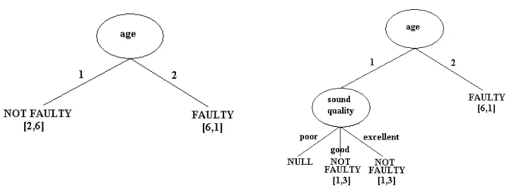
Figure 4 presents a cost-sensitive decision tree induced by applying the EG2 algorithm to the

(32)

[image:32.595.192.380.92.342.2]

24

Figure 4Decision tree after EG2 has been applied to the dataset in Table 1

Algorithms that continue this adaptation of information theoretic measures but also take account of the misclassification cost as well as the test costs include an approach by Ni et al. (2005), Zhang et al. (2007), Zhang (2010) and Liu (2007). Although the detailed measures differ, they all aim to capture the trade-off between the cost of acquiring the data and its contribution to reducing misclassification cost. Ni et al. (2005), for example, utilize the following attribute selection measure:

Performance: 12 = (3245(675*'− 19 ∗ ;1/(1+ 1)) ∗ _ώ _(3.6) where ώA is the bias of experts for attribute A and DMCA is the improvement in misclassification cost if the

attribute A is used.

(33)

25 of an attribute this bias is set to the default value of 1. If some attributes produce the same value for equation (3.6), preference is given to those attributes with the largest reduction in misclassification costs (DMCA). If this fails to find an attribute then the attribute with the

largest test cost (CA) is chosen as the aim is to reduce misclassification costs.

Liu (2007) identifies some weaknesses of equation (3.6), noting that several default values have been used, so develops the PM algorithm. Liu (2007) notes that if gain ratios of

attributes are small, the values returned by the original algorithm, equation (3.6), would be small; resulting in the costs of attributes being ignored. If attributes have large total costs, the information contained in those attributes will be ignored. Other issues are the conflict of applying resource constrains. For instance, the overall aim of this algorithm is to allow for user resource constrains and it is therefore necessary to allow for the fact that users with increased test resources are not concerned as much about the cost of attributes, rather in the reduction of misclassification costs, and alternatively those with limited test resources are more concerned with the cost of the tests in order to reduce the overall costs rather than only reducing the misclassification costs.

In order to trade off between these needs, a solution offered by Liu (2007) is to normalize the gain ratio values and to employ a harmonic mean to weigh between concerns with test costs (low test resources) and reduction in misclassification costs (when test resources are not an issue), additionally a parameter α is used to balance requirements of different test examples

with different test resources.

Zhang et al. (2007) take a different approach when adapting the Performance algorithm.

(34)

26 same scale; test costs would be considered on a cost scale of currency whilst misclassification costs, particularly in terms of medical diagnosis, states Zhang et al. (2007), must be a social issue; what monetary value could be assigned for potential loss of life? The adaptation attempts to achieve maximal reduction in misclassification costs from lower test costs. The only difference to equation (3.6) to produce CTS (Cost-Time Sensitive Decision Tree), is to

remove the bias of expert parameter, preferring to address such issues as waiting costs (also referred to in other studies as delayed cost), at the testing stage by developing appropriate test strategies.

The above measures all utilize the information gain as part of a selection measure. An alternative approach, taken by Breiman et al. (1984), is to alter the class probabilities, P(i) used in the information gain measure. That is, instead of estimating P(i) by Ni/N, it is weighted by the relative cost, leading to an altered probability (Breiman, et al. 1984, p114):

Altered Probabilityi = Cij*(Ni/N) / ∑j cost(j)(Nj/N) (3.7)

In general, the cost of misclassifying an example of class j may also depend on the class i that

it is classified into, so Breiman et al. (1984) suggest adopting the sum of costs of misclassification:

cost(j) = ∑i Cij (3.8)

(35)

27 Altered GINI = 1-∑ky=1 Altered Probabilityy2 (3.9)

C4.5 allows the use of weights for examples, where the weights alter the Information Gain measure by using sums of weights instead of counts of examples. So instead of counting the number of examples with attribute value a and class k, the weights assigned to these

examples would be summed and used in equation (2.1).

C4.5’s use of weights has been utilized to incorporate misclassification costs, by overriding the weight initialization method. For example if the cost to misclassify a faulty example from the example dataset in Table 1 is 5, those examples belonging to class ‘faulty’ could be allocated the weight of 5, and examples belonging to class ‘not faulty’ could have the weight of 1, so that more weight is given to those examples with the higher misclassification cost.

C4.5CS is one such algorithm which utilizes this use of weights.

The method of computing initial weights by C4.5CS is similar to that of the

GINIAlteredPriors algorithm developed by Breiman et al. (1984) and Pazzani et al. (1994).

When presented with the same dataset, both methods would produce the same decision tree. However Ting (1998) observes that the method which alters the priors would perform poorly as pruning would be carried out in a cost insensitive way, whereas the C4.5CS algorithm uses

the same weights in its pruning stage. In his experiments with a version which replicates Breiman et al. (1984)’s method, C4.5(π’) performs worse that the C4.5CS algorithm. He

(36)

28 The sum of all the weights for class j in the C4.5CS algorithm will be equal to N. The aim of

C4.5CS is to reduce high cost errors by allocating the highest weights to the most costly

errors so that C4.5 concentrates on reducing these errors.

C4.5CS (Ting 1998, 2002):

+-"ℎ%_> = ?%(@)_{∑ *B7(5)A}A

C

C (3.10)

where cost(j) and cost(i) are as defined by equation (3.8).

MaxCost (Margineantu and Dietterich 2003): +-"ℎ%_> = DE_FG5GH 1_>5 (3.11)

AvgCost (Margineantu and Dietterich 2003): +-"ℎ%_> = ∑ IC J CKL,CNI

(HOF) (3.12)

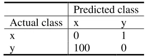
These latter two algorithms have been designed to solve multi-class problems so the cost matrices involved are not the usual 2 x 2 grids presented when solving two class problems. Instead a k x k matrix is used, the diagonal cells containing the cost of correctly classifying an

example, usually zero although for some domains it could well be greater than zero.

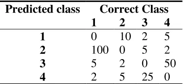
Table 5 presents an example of a cost matrix of a dataset where k = 4. The diagonal cells have

been assigned zero therefore a correct classification results in zero cost. Two algorithms developed by (Margineantu and Dietterich 2003) use this cost matrix directly to compute initial weights. MaxCost uses the worst case cost of misclassifying an example. The

maximum value within a column is considered to be the worst case cost of misclassifying an example. For instance, the weight of all class 1 examples will be assigned 100 as that is the maximum misclassification cost in the column corresponding to class 1. AvgCost calculates

(37)

29 examples are assigned 35.6. These two algorithms are considered more efficient than others of this type (Margineantu and Dietterich 2003).

Predicted class Correct Class

1 2 3 4

1 0 10 2 5

2 100 0 5 2

3 5 2 0 50

[image:37.595.205.391.168.254.2]

4 2 5 25 0

Table 5 Example of a cost matrix of a four class problem

Margineantu and Dietterich (2003) also suggest an alternative way of setting the weights, called EvalCount, where an accuracy-based decision tree is first induced and then used to

obtain the weights. The training data is sub divided into a sub training set and a validation set. The sub training set is then used to grow an accuracy based decision tree. Using this decision tree, the cost of misclassification for each class on the validation set is then measured using the cost matrix. The weight allocated to a training example is then set to the total cost of misclassifying an example of that class.

3.1.1.2 Direct use of costs. Instead of adapting the information gain to include costs, a number of algorithms utilize the cost of misclassification directly as the selection criteria. These algorithms can be subdivided into two groups: those that only use misclassification costs and those which also include test costs.

(38)

30 examples. Of course, if none of the attributes results in a reduction, then a leaf node is created.

Cost-Minimization (Pazzani et al. 1994), Decision Trees with Minimal Cost (Ling et al. 2004)

and two adaptations Decision Trees with Minimal Cost under Resources Constrain (Qin et al.

2004) and CSTree (Ling et al. 2006a) use either misclassification costs or a combination of

misclassification costs and test costs to partition the data. Cost-Minimization, the simplest of

these chooses the attribute which results in the lowest misclassification costs.

One of the main algorithms to use costs directly in order to find the attribute on which to partition data, is Decision Trees with Minimal Cost developed by Ling et al. (2004),

spawning other adaptations. Expected cost is calculated using both misclassification costs and test costs aiming to minimize the total cost. An attribute with zero or smallest test cost is most likely to be the root of the tree, thus attempting to reduce the total cost. This algorithm has been developed firstly to minimize costs and secondly to deal with missing values in both the training and testing data. In training, examples with missing values remain at the node representing the attribute with missing values. In a study comparing techniques by Zhang et al. (2005), it was concluded that this was the best way to deal with missing values in training examples. How and whether to obtain values during testing are solved by constructing testing strategies and are discussed additionally in Ling et al. (2006b).

To illustrate what happens when only the costs (i.e., no information gain) are used to select attributes, consider the application of the DT with MC algorithm to the examples in Table 1,

(39)

31

[image:39.595.104.464.81.218.2]

5(a) Tree from DT with MC 5(b) Tree if left branch is expanded.

Figure 5Decision tree when DT with MC has been applied to dataset in Table 1

Figure 5(a) shows the tree induced by DT with MC algorithm, which is very different from

the cost-sensitive tree produced by EG2 (Figure 4) and from the tree produced by ID3 (Figure

1). This algorithm employs pre-pruning, that is, it stops splitting as soon as there is no improvement. Figure 5(b) shows a partial tree obtained, if the left branch was expanded further. The additional attribute that would lead to the least cost is sound quality, with a total cost of 220 units since there are still two faulty examples misclassified but there is the extra cost of 120 units for testing Sound Quality (i.e., 8 examples each costing 15 units). However, the cost without splitting is 100 units (i.e., 2 faulty examples misclassified, with misclassification cost of 50) and hence, in this case, the extra test is not worthwhile.

(40)

32 Ling et al. (2004)’s algorithm is further adapted into CSTree which does not take into account

test costs, using only misclassification costs (Ling et al. 2006a). CSTree deals with two-class

problems and estimates the probability of the positive class using the relative cost of both classes and uses this to calculate expected cost.

A different and perhaps more extensive idea is by Qin et al. (2004), who develop an adaptation of the Ling et al. (2004) algorithm Decision Trees with Minimal Cost under

Resource Constrains. Its purpose is to trade off between target costs (test costs and

misclassification costs) and resources. Qin et al. (2004) argue that it is hard to minimize two performance metrics and it is not realistic to minimize both of them at the same time. So they aim to minimize one kind of cost and control the other in a given budget. Each attribute has two costs, test cost and constrain, likewise each type of misclassification has a cost and a constrain value. Both these values are used in the splitting criteria, to produce a target-resource cost decision tree (Qin et al. 2004) and used in tasks involving target cost minimization (test cost) and resources consumption for obtaining missing data.

Decision Tree with Minimal Costs under Resource Constrain:

ICFS = (T − TA) 1#?%."#⁄ (3.13)

1#?%."# = (W − ) ∗ .+ X ∗ 15>(.) + # ∗ 1>5(.) + ∗ 1>5(.) (3.14)

here T is the misclassification cost before splitting, TA is the expected cost if attribute A is chosen, rA, Cij(r) and

Cji(r) are the resource costs for false negatives and false positives respectively, p is the number of positive examples and n the number of negative examples and o the number of examples with missing attribute value.

A different approach than simply using the decision tree produced using direct costs, is suggested by Sheng and Ling (2005), a hybrid cost-sensitive decision tree. They develop a hybrid between decision trees and Naïve Bayes, DTNB (Decision Tree with Naïve Bayes).

(41)

33 classifying, originally known attribute values not appearing in the path taken by a test example. It is argued by Sheng and Ling (2005) that any value is available at a cost, if values are available at the testing stage, these might be useful in order to reduce misclassification costs and to ignore them would be wasting available information. Naïve Bayes can use all known attribute values for classification but has no structure to determine which tests to perform and in what order should they be carried out in order to obtain unknown attribute values. The DTNB algorithm aims to combine the advantages of both techniques.

A decision tree is built using expected cost reduction using the sum of test costs and expected misclassification costs to determine whether to further split the data and on what attribute. Simultaneously a cost-sensitive Naïve Bayes model using Laplace correction and misclassification costs is hidden at all nodes including leaves and is used for classification only of the test examples. The decision tree supplies the sets of tests used in various test strategies and the Naïve Bayes model, built on all the training data, classifies the test examples, thus overcoming problems caused by segmentation of data, that is the reduction of data at lower leaves, and making use of all attributes with known values but which have not been selected during induction so that no information once obtained, is wasted. In experiments, this hybrid method proved to be better in combination than the individual techniques (Sheng and Ling 2005).

3.1.1.3 Linear and non-linear decision nodes. Most of the early algorithms handle numeric

(42)

34 induction process and the primary difference between them, which we summarize below, is whether they adopt linear or non-linear splits and how they obtain the splits.

The LMDT algorithm (Draper et al. 1994) was one of the first to go beyond axis-parallel

splits. This algorithm aims to develop a decision tree whose nodes consist of Nilsson’s (1965) linear machines. A linear machine aims to learn the weights of linear discriminants. Before looking at the LMDT algorithm, it is worth understanding the concept of a linear machine,

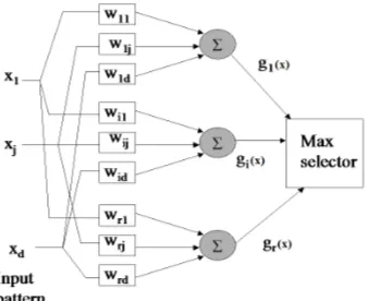
which is central to the LMDT algorithm. The following figure summarizes the structure of a

linear machine.

Each function gi(x) aims to represent a class i in a winner takes all fashion. A weight wij represents the coefficient of xj for the ith linear discriminant function. The training procedure

involves presenting an example x that belongs to a class i. If the example is misclassified,

say into class j, then the weights of the jth machine can be decreased and the i th machine

increased, i.e.:

Wi = Wi + c.x

Wj = Wj - c.x (3.15)

[image:42.595.213.382.595.733.2]

where c is a correction factor, and the Wi _{and W}j_{are the weight vectors for the i}th _{and j}th _{linear discriminants.}

(43)

35 When the classes are linearly separable, the use of a constant correction rate (i.e. as in a perceptron) is sufficient to determine a suitable discriminant and this simple procedure converges. However, in general, the classes may not be linearly separable and the above procedure may not converge. Draper et al. (1994) overcame this problem by utilizing a thermal training procedure developed by Frean (1990). This involved using an annealing

parameter β to determine the correction factor c as follows:

c = β2 / β + k where k = (Wj – Wi)T x / 2xT x. (3.16) where Wj is the weight vector of the ith discriminant function that represents

the true class of the example, and Wj is the weight vector of the jth discriminant

function that represents the class in which the example is misclassified.

LMDT is altered to make it cost-sensitive by altering its weight learning procedure, with the

aim of reducing total misclassification costs. In the modified version, it samples the examples based on the cost of misclassifications made by the current classifier. The training procedure is initialized for each class using a variable ‘proportioni’, for each class i. Next, if the

stopping criterion is not met, the thermal training rule trains the linear machine and if the examples have been misclassified, the misclassification cost is used to compute a new value for each ‘proportioni’.

An alternative approach to obtaining linear splits, taken in the LDT system (Vadera 2005b),

is to take advantage of discriminant analysis which enables the identification of linear discriminants of the form (Morrison 1976; Afifi and Clark 1996):

(YF− Y )ΣOFE −F(Y_F− Y )ΣOF(Y_F+ Y ) ≤ ln \]L^(])

(44)

36 Theoretically, it can be shown that equation (3.17) minimizes the misclassification cost when ` has a multivariate normal distribution and when the covariance matrices for each of the two

groups are equal.

This trend of moving towards more expressive divisions is continued in the CSNL system

(Vadera 2010) that adopts non-linear decision nodes. The approach also utilizes discriminate analysis, and adopts following split that minimizes cost provided the class distributions are multivariate normal:

−FE7_{(∑ −}OF

F ∑ )E + (YOF F7∑ −OFF Y7∑ )E − a ≥ ln \OF _L]]L^(_^(]_L)₎_

a = F# (| ∑ |L

| ∑ |] ) +

F_(Y

F7∑ YOFF F− Y 7∑ YOF ) (3.18)

where x is a vector representing the example to be classified, µ1, µ2 are the mean vectors for the two classes, ∑1,

∑2 are the covariance matrices for the classes and ∑1-1, ∑2-1 the inverses of the covariance matrices.

Given that the multivariate assumption may not hold in practice, it may be that utilization of a subset of variables could lead to more cost-effective splits, and hence several strategies for subset selection are explored. One strategy, explored in Vadera (2005a), is to attempt all possible combinations and select the subset that minimizes cost. However, this strategy is not particularly scalable and results in trees that are difficult to visualize. An alternative strategy, explored in (Vadera 2010), selects two of the most informative features, as measured by information gain, and uses the above equation (3.18) to obtain non-linear divisions.

3.1.2 Post construction

(45)

37 costs. Hence, various authors have explored how misclassification costs can be applied after a tree has been constructed.

One of the simplest of ways is to change how the label of the leaf of the decision tree is determined. I-gain Cost-Laplace Probability (Pazzani et al. 1994) uses a Laplace estimate of

the probability of a class given a leaf shown in equation (3.19). If there are Ni examples of class i at a leaf and k classes then the Laplace probability of an example being of class i is:

(") = ACc F

Hc ∑JdKLAd (3.19)

When considering accuracy only, an example is assigned to the class with the lowest expected error. To incorporate costs, the class which minimizes the expected cost of misclassifying an example into class j is selected, where the expected cost is defined by:

EX-%-e 1?% / ;"???"/"%"# "#% ?? @ = ∑ 1₅ _5>(") (3.20)

(46)

38 The convex hull created from the points (0,0), the four classifiers and (1,1) represents an optimal front. That is, for any classifier below this convex hull, there is a classifier on the front that is less costly.

Figure 7 Example ROC

The idea behind Ferri et al. (2002)’s approach is to generate the alternative classifiers by considering all possible labellings for the leaf nodes of a tree. For a tree with m leaf nodes,

and a two class problem, there are 2m alternative labels, which could be computationally expensive. However, Ferri et al. (2002) shows that for a two class problem, if the leaves are ordered by the accuracy of one of the classes, then only m+1 alternative labellings are

needed to define the convex hull, where the jth node of the ith labelling, Li,j, is defined by:

f5,> = g−h- "/ @ < "_{+h- "/ @ ≥ "}j (3.21)

(47)

39

3.2 Multiple tree, non-greedy methods for cost-sensitive decision tree induction

Greedy algorithms have the potential to suffer from local optima, and hence an alternative direction of research has been to develop algorithms that generate and utilize alternative trees. There are three common strands of work: Section 3.2.1 describes the use of genetic algorithms, Section 3.2.2 describes methods for boosting and bagging, and Section 3.2.3 describes the use of stochastic sampling for developing anytime and anycost frameworks.

3.2.1 Use of Genetic Evolution for Cost-Sensitive Tree Induction

Several authors have proposed the use of genetic algorithms to evolve cost-effective decision trees (Turney 1995). Just as evolution in nature uses survival of the fittest in order to produce next generations, a pool of decision trees are evaluated using a fitness function, the fittest retained and combined to produce the next generation repeatedly until a cost-effective tree is obtained. This section describes the algorithms that utilize evolution, which vary in the way they represent, generate, and measure the fitness of the trees.

One of the first systems to utilize GAs was Turney’s (1995) ICET system (Inexpensive

Classification with Expensive Tests. ICET uses C4.5 but with EG2’s cost functionto produce

decision trees, in Section 3.1.1.1.

(48)

40

ICET begins by dividing the training set of examples into two random but equal parts: a

sub-training set and a sub-testing set. An initial population is created consisting of individuals with random values of CAi, ω, and CF. C4.5, with the EG2’s cost function, is then used to generate a decision tree for each individual. These decision trees are then passed to a fitness function to determine fitness. This is measured by calculating the average cost of classification on the sub-testing set.

The next generation is then obtained by using the roulette wheel selection scheme, which selects individuals with a probability proportional to their fitness. Mutation and crossover are used on the new generation and passed through the whole procedure again. After a fixed number of generations (cycles) the best decision tree is selected. ICET uses the GENEtic

Search Implementation System (GENESIS, Grefenstette (1990)) with its default parameters including a population size of 50 individuals, 1000 trials and 20 generations.

More recently, Kretowski and Grześ (2007) describe GDT-MC (Genetic Decision Tree with

Misclassification Costs), an evolutionary algorithm in which the initial population consists of

decision trees that are generated using the usual top down procedure, except that the nodes are obtained using a dipolar algorithm. That is, to determine the test for a node, first two possible examples from the current dataset are randomly chosen such that they belong to different classes. A test is then created by randomly selecting an attribute that distinguishes the two examples. Once a tree is constructed, it is pruned using a fitness function. The fitness function used in GDT-MC aims to take account of the expected misclassification cost as well

(49)

41 2"%#-?? / %.-- = \1 −_lk_ (1 + m. no) (3.22)

where EC is the misclassification cost per example, MC is the maximal possible cost per example, TS is the number of nodes in the tree and γ is a user provided parameter that determines the extent to which the genetic algorithm should minimize the size of the tree to aid generalization.

The genetic operators are similar in principle to the cross-over and mutation operators, except that they operate on trees. Three cross-over like operators are utilized on two randomly selected nodes from two trees:

• exchange the sub-trees at the two selected nodes.

• if the types of tests allow, then exchange just the tests.

• exchange all sub-trees of the selected nodes, randomly selecting the ones to be

exchanged.

The mutation operators adopted allow a number of possible modifications of nodes, including replacing a test with an alternative dipolar test, swapping of a test with a descendent node’s test, replacement of a non-leaf node by a leaf node, and development of leaf node into a sub-tree. A linear ranking scheme, coupled with an elitist selection strategy, is utilized to obtain the next generation (Michalewicz 1996).3

The ECCO (Evolutionary Classifier with Cost Optimisation) system (Omelian 2005) adopts

a more direct use of genetic algorithms by mapping decision trees to binary strings and then adopting the standard cross-over and mutation operators over binary strings. Attributes are represented by a fixed size binary string, so for example 8 attributes are coded with 3 bits. Numeric attributes are handled by seeking an axis parallel threshold value that maximizes

3_{The elitist strategy ensures that a few of the fittest are copied to the new generation, and the linear ranking strategy}

(50)

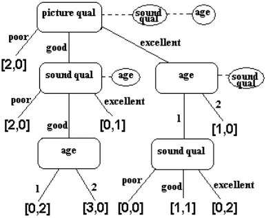
42 information gain, thereby resulting in a binary split. The mapping between a tree and its binary string is achieved by assuming a fixed size maximal tree where each node is capable of hosting an attribute which has the most features.4 Figure 8 illustrates the mapping for a problem where the attributes have two features only. Such a maximal tree is then interpreted by mapping the nodes to attributes, assuming that the branches are ordered in terms of the features. In addition, mutation may result in some nodes with non-existent attributes, which are also translated to decision nodes.

A tree is then populated with the examples in a training set and each leaf node labelled with a class that minimizes the cost of misclassification. A version of the minimum error pruning algorithm that minimizes cost instead of error is used for pruning. The fitness measure used is the expected cost of classification, taking account of both the cost of misclassification and the cost of the tests. Once genes are mapped to decision trees and pruned, and their fitness obtained, the standard mutation and cross-over operators applied, a new generation of the fittest is evolved and the process repeated a fixed number of cycles. Like ICET, ECCO

adopts the GENESES GA system and adopts its default parameters.

Figure 8 Illustration of mapping

(51)

43 Li et al. (2005) take advantage of the capabilities of Genetic Programming (GP), which enable representation of trees as programs instead of bit strings, to develop a cost-sensitive decision tree induction algorithm. They use the following representation of binary decision trees as programs, defined using BNF (Li et al. 2005):

<Tree> :: “if-then-else” <Cond><Tree><Tree> | Class

| Not <Cond> | Variable<RelationOperation>Threshold RelationOperation ::= “>” | “<” | “=”

Unlike GDT-MC, which utilizes specialized mutation and crossover operators, Li et al.

(2005) adopt the standard mutation and crossover operators of genetic programming. A tournament selection scheme, in which four individuals are selected randomly with a probability proportional to their fitness, compete to move to the next generation. The fittest of the four is copied to the pool for the next generation and this tournament process repeated to produce the complete mating pool for the next generation. The fitness function employed is also different from ICET, ECCO and GDT-MC. Unlike, these methods, which utilize

expected cost, Li et al (2005) propose the following fitness function that is based on the principle that a cost-effective classifier will maximize accuracy (RC) but minimize the false positive rate (RFP):

(52)

44 Experimentation with this function leads them to the following additional constraint to ensure that accuracy of one of classes is not compromised when the costs of misclassifications are significantly imbalanced:

Wrc = 1 if C+ϵ (Pmin, Pmax), 0 otherwise, (3.24) where C+ is the proportion of examples predicted to be positive, and the Pmin and Pmax define the expected range

for C+ that is provided by a user.

3.2.2 Wrapper methods for cost-sensitive tree induction

A significant amount of research has been done on accuracy based classifiers, and instead of developing new cost-sensitive classifiers or adapting them as described above, an alternative strategy is to develop wrappers over accuracy based algorithms.

This section describes two approaches for utilizing existing accuracy based algorithms. Section 3.2.2.1 describes methods based on boosting, where an accuracy based learner is used to generate an improving sequence of hypotheses and Section 3.2.2.2 describes methods based on bagging that are based on generating and combining independent hypotheses. Section 3.2.2.3 describes a method which implicitly includes alternative hypotheses but in one structure.

3.2.2.1 Cost-Sensitive Boosting. Boosting involves creating a number of hypotheses htand then

combining them to form a more accurate composite hypothesis of the form (Schapire 1999; Meir and Rätsch 2003):

/(E) = ∑ pq7rF 7ℎ7(E) (3.25)