Si m ul a ti n g a c o u s ti c s c a t t e r i n g
fr o m a t m o s p h e r i c t e m p e r a t u r e
fl u c t u a ti o n s u si n g a k-s p a c e
m e t h o d
H a r g r e a v e s , JA, Ke n d ri c k, P a n d vo n H ü n e r b e i n , S
h t t p :// dx. d oi.o r g / 1 0 . 1 1 2 1 / 1 . 4 8 3 5 9 5 5
T i t l e
Si m u l a ti n g a c o u s ti c s c a t t e r i n g f r o m a t m o s p h e r i c
t e m p e r a t u r e flu c t u a ti o n s u si n g a k-s p a c e m e t h o d
A u t h o r s
H a r g r e a v e s , JA, Ke n d r i c k, P a n d vo n H ü n e r b ei n , S
Typ e
Ar ticl e
U RL
T hi s v e r si o n is a v ail a bl e a t :
h t t p :// u sir. s alfo r d . a c . u k /i d/ e p ri n t/ 3 0 7 6 0 /
P u b l i s h e d D a t e
2 0 1 4
U S IR is a d i gi t al c oll e c ti o n of t h e r e s e a r c h o u t p u t of t h e U n iv e r si ty of S alfo r d .
W h e r e c o p y ri g h t p e r m i t s , f ull t e x t m a t e r i al h el d i n t h e r e p o si t o r y is m a d e
f r e ely a v ail a bl e o nli n e a n d c a n b e r e a d , d o w nl o a d e d a n d c o pi e d fo r n o
n-c o m m e r n-ci al p r iv a t e s t u d y o r r e s e a r n-c h p u r p o s e s . Pl e a s e n-c h e n-c k t h e m a n u s n-c ri p t
fo r a n y f u r t h e r c o p y ri g h t r e s t r i c ti o n s .
Simulating acoustic scattering from atmospheric temperature
fluctuations using a
k
-space method
Jonathan A. Hargreaves,a)Paul Kendrick, and Sabine von Hunerbein€
Acoustics Research Centre, The University of Salford, Manchester M5 4WT, United Kingdom.
(Received 3 May 2013; revised 5 November 2013; accepted 8 November 2013)
This paper describes a numerical method for simulating far-field scattering from small regions of inhomogeneous temperature fluctuations. Such scattering is of interest since it is the mechanism by which acoustic wind velocity profiling devices (Doppler SODAR) receive backscatter. The method may therefore be used to better understand the scattering mechanisms in operation and may eventually provide a numerical test-bed for developing improved SODAR signals and post-processing algorithms. The method combines an analytical incident sound model with a k-space model of the scattered sound close to the inhomogeneous region and a near-to-far-field transform to obtain far-field scattering patterns. Results from two test case atmospheres are presented: one with periodic temperature fluctuations with height and one with stochastic temperature fluctuations given by the Kolmogorov spectrum. Good agreement is seen with theoretically predicted far-field scattering and the impli-cations for multi-frequency SODAR design are discussed. VC 2014 Acoustical Society of America
[http://dx.doi.org/10.1121/1.4835955]
PACS number(s): 43.28.Js, 43.28.Gq, 43.20.Fn, 43.20.Px [VEO] Pages: 83–92
I. INTRODUCTION
Sound Detection and Ranging (SODAR) devices mea-sure the backscattering of sound pulses transmitted into the lower atmosphere, allowing remote sensing of a variety of data including inversion layers and vertical profiling, wind speed, wind direction, turbulence quantities and stability classes.1 Unlike direct measurement techniques (such as mast anemometers), they are quick to deploy and provide continuous data with height; hence, they find application in atmospheric research, pollution monitoring, and wind-energy surveying.
In profiling the lower atmosphere using SODAR, one may encounter difficulties with range and velocity resolution as well as signal to noise ratio problems. To improve the ac-curacy of these parameters, new signals and analysis meth-ods need to be evaluated. This is difficult to achieve by experimentation, however, since the “true” atmospheric data required for comparison is not available and must be acquired either from similar instruments or other devices with their own limitations. Thus, there is a requirement for a SODAR simulator to inform on SODAR performance char-acteristics over a range of atmospheric conditions and this paper presents some initial steps toward that objective. In addition, it studies whether the process causing the backscat-ter is compatible with the matched-filbackscat-ter post-processing required for multi-frequency “pulse compression” SODAR signals.2,3These have been proposed to overcome the usual tradeoff between transmitted power and height resolution by transmitting multiple pulses of different frequencies.
Atmospheric scattering from acoustic pulses is strongest where the spacing of the scattering structures is related to in-teger multiples of half a wavelength; the mechanism in
operation here is Bragg scattering, though it has also been called “Acoustic Iridescence” in other applications.4 Previous models of wind profilers have not simulated the scattering process directly but have been based on statistical models of the effective cross-section of sound scattering in the atmosphere,1,5–7ensemble average spectra of backscat-tered sound,8or frequency modulation of a pure tone by a simulated velocity profile.9In contrast, numerical algorithms such at Finite-Difference-Time-Domain (FDTD) can directly model the scattering of these transient acoustic pulses by a specific temperature and velocity distribution.10–12 Given however that SODARs generally operate in the frequency range 1000–5000 Hz and generally have a range of 100 m upward, FDTD simulation of the entire scattering volume in three dimensions is unfortunately not feasible with currently available computing power.
The classical theory studies the scattering from a region of turbulence within an otherwise homogeneous atmosphere (for example, see Ref. 7, Sec. 7.1.1). The distance from the scattering volume to the sound source and receivers is assumed to be large with respect to the characteristic size of the volume, so the incident sound wave is approximately a plane wave and a far-field approximation may also be applied to the scattered sound at the receivers. Cheinet et al.13 recently studied this scenario numerically in two dimensions (2D) using FDTD. Good agreement with the classical theory was seen for large scattering angles and the discrepancies at small scattering angles could be explained by approximations introduced in the classical theory.
In this paper, a similar numerical study is conducted in three dimensions (3D), but requires a hybrid approach due to the significantly increased storage and computation require-ments that 3D presents. In particular, it was possible for the authors of Ref.13to model in 2D (using a cluster) a domain large enough that the receivers could be placed in the far-field relative to the scattering volume and the far-field a)Author to whom correspondence should be addressed. Electronic mail:
scattering calculated directly. In contrast, the algorithm reported herein was both in 3D and designed to run on a sin-gle workstation, so the volume modeled using FDTD had to be restricted to be only slightly larger than the turbulent region. This meant far-field pressure could not be estimated directly from the grid data and instead a Near-To-Far-Field (NTFF) transform14 was applied to convert the data at the edge of the grid into far-field pressure. Since the NTFF trans-form should operate only on the scattered sound, it was also necessary to separate the incident and scattered fields. Separate modeling of incident and scattered sound waves is not uncommon in acoustic and electromagnetic simulation of scattering from impenetrable objects15 (see “scattered field” formulation Sec. 5.10), but its application to scattering by a region of inhomogeneous refractive index is believed to be novel.
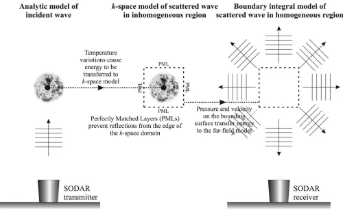
The structure of the complete algorithm is depicted in Fig.1, showing its three parts (which are spatially coincident but depicted separately for clarity). On the left is the incident sound model; this is stated analytically and propagates through V unchanged. In the middle is the scattered sound model in V; this provides a correction such that the total sound respects the inhomogeneous refractive index of V. Finally, on the right is the far-field scattered sound model, computed using the NTFF transform over a surface which is within the FDTD modeling domain but which also entirely encloses V. Compared to a total-field model of the entire atmosphere, this approach has the benefits of reduced com-putational cost, since it avoids using an expensive volumetric method to model the homogeneous part of the atmosphere,
and better use of floating point precision, since the incident and scattered sound waves (which typically differ by many orders of magnitude) are computed separately so “subtraction error” will not occur.
The numerical method is described in detail in Sec. II
and the results of the numerical simulations are presented in Sec. III. Sec. IVsummarizes the findings of the paper, dis-cusses the scope of the model and identifies future directions.
II. NUMERICAL METHOD
Consider the problem of a scattering volumeV with an inhomogeneous temperature profileTð Þr , whereris a vector representing position in 3D Cartesian space, within an other-wise homogenous atmosphere with temperature T0, density q0, and sound speed c0. Density and sound speed within V
may be found byqð Þ ¼r q0T0=Tð Þr andcð Þ ¼r c0
ffiffiffiffiffiffiffiffiffiffiffiffiffiffiffiffi Tð Þr=T0
p
, respectively, on the assumption that the ambient pressure is constant and the air is dry and obeys the ideal-gas law. It is assumed that the medium is stationary except for the small perturbations due to acoustic particle velocity (i.e., no wind or medium velocity due to turbulence).
An incident sound wave, which satisfies the wave equa-tion withq0andc0, propagates upward through the
homoge-neous atmosphere. As it impinges on V, the variations in density and sound speed cause changes in how the sound wave propagates, modifying its shape. Figure2illustrates an exaggerated case of this where the temperature in V (area within dotted circle) is significantly lower than T0, causing
the sound wave to slow down. Rather than modify the
[image:3.612.58.558.415.722.2]incident sound wave [Fig. 2(a)], the algorithm instead introduces a scattered sound wave [Fig.2(b)] such that the sum of these gives a total sound wave [Fig. 2(c)], which satisfies the wave equation with qð Þr and cð Þr. This includes cancellation of the incident and scattered wave-fronts immediately above the cold region such that “slowing” of the total wave can be observed. Ultimately, it is desirable to know the directivity with which this scat-tered sound wave propagates into the far-field after it leavesV; this is calculated using a boundary integral over a surface enclosingV.
A. Incident sound model
The homogeneous incident sound wave is chosen to be a plane wave with its propagation direction described by the unit vector k^i and time variation by the function fð Þs. Its pressurepiand particle velocityuiare given by
piðr;tÞ ¼f tk^ir=c0
; (1)
uiðr;tÞ ¼k^ipiðr;tÞ=q0c0: (2)
These satisfy the first-order linearized equations for a homo-geneous medium
q0 @ui
@t ¼ rpi; (3)
@pi
@t ¼ q0c
2
0r ui: (4)
B. Scattered sound model
The scattered sound wave has pressure ps and particle velocityus. Below are the first order linearized equations for an inhomogeneous medium [e.g., Ref. 13 Eq. (1) and Eq.
(2), omitting source and medium velocity terms], which apply to the total pressurept¼piþpsand total particle ve-locityut¼uiþusinsideV,
qð Þr @ut
@t ¼ rpt; (5)
@pt
@t ¼ qð Þrc
2
r
ð Þr ut: (6)
These are split into the incident and scattered parts
qð Þr @ui
@t þ
@us
@t
¼ rð piþ rpsÞ; (7)
@pi
@t þ
@ps
@t ¼ qð Þrc
2ð Þ r r u
iþ r us
ð Þ: (8)
Subtracting Eq. (3) from Eq. (7) and Eq. (4) from Eq. (8)
gives the equations to be modeled numerically
qð Þr @us
@t ¼ rpsþðq0qð ÞrÞ
@ui
@t ; (9)
@ps
@t ¼ qð Þrc
2ð Þr r u
sþ q0c
2
0qð Þrc 2ð Þr
r ui
¼ q0c20r us: (10)
It should be noted thatpsandus include multiple scattering
as well as compensation for the first-order scattering that pi and ui should experience due toqð Þr andcð Þr ; Eq.(9) and
Eq. (10)are exact results. The simplification in the second line of Eq. (10)is possible becauseqð Þr c2ð Þ ¼r q
0c20 when
only temperature fluctuations are present, hence the incident term equates to zero and may be omitted. From the perspec-tive of the scattered sound model the term@ui=@tin Eq.(9)
is like a distributed source, passing sound energy from the incident sound model to the scattered sound model such that the total sound (sum of incident and scattered) satisfies the inhomogeneous medium properties inV.
C. k-space algorithm
For an incident plus scattered sound model to operate correctly, it is crucial that the speed of wave propagation is identical in both models; if not, then sound energy being transferred from the incident to scattered model in the cur-rent time-step will be misaligned with scattering from previ-ous time-steps. This is automatically assured in typical “scattered field” FDTD formulations, since a FDTD scheme is also used for the incident sound. However, further consid-eration is required here because the incident sound wave is stated analytically. Standard FDTD algorithms suffer from the well reported issue of numerical dispersion (e.g., Ref.15, Chap. 4), meaning the speed of wave propagation is direc-tion and frequency dependent, so they are unsuitable for this application. Here instead the scattered field in the homoge-neous volume will be evaluated using a k-space variant of the FDTD method.16 This is closely related to the Pseudo-Spectral-Time-Domain (PSTD)17 method and uses a spatial
FIG. 2. (Color online) Example of the incident plus scattering model of a cold temperature region (inside the dashed circle) within a uniform temperature medium. Arrows indicate wave propa-gation direction and color scale is iden-tical across all three subplots. (a) incident pressure; (b) scattered pressure; (c) total pressure (incidentþscattered).
Fourier series to interpolate the grid data at each time-step, allowing the spatial derivatives to be found by Fast Fourier Transform (FFT) using fewer grid points per wavelength than would be required by a finite-difference scheme of simi-lar precision. Crucially for the application herein, numerical dispersion effects are compensated for in thek-space spatial operators (see Ref.16, Sec. II), so the resulting algorithm is free of numerical dispersion.
The algorithm used here has been adapted from Tabei et al.16and thek-wave toolbox18 with the following primary differences: inclusion of the extra incident sound terms above, absence of relaxation absorption, and the use of collocated (non-staggered) grids. Use of collocated grids is known to cre-ate spatial Gibbs effects for sudden changes in medium proper-ties, but those are not present in the atmospheric temperature profiles under consideration so the algorithm can benefit from a slightly simpler NTFF implementation and the potential to support velocity fluctuations in future (these involve spatial tensor derivatives which are complicated to implement on staggered grids). The pressure and particle velocity grids are however still staggered in time. For a collocated grid scheme thek-space differential operators, including dispersion correc-tion, are given by the following concatenation of operators, where F represents a multi-dimensional FFT and F1 its
inverse. HereDtis the time-step duration,kis the spatial wave number in thek-domain (for more details see Ref.16) andkx is its component in thexdirection. Note that for brevity only thexdirection operators are given in what follows, but equiva-lent statements exist foryandz,
@
@xf…g F
1
ikxsincðc0Dtk=2ÞFf…g
n o
: (11)
The collocated grid algorithm was verified against the stag-gered algorithm implemented in the k-wave toolbox by marching on from initial conditions, and the error between the two algorithms was found to be less than 50 dB com-pared to the excited pressure in the medium.
The modeling region is surrounded by a Perfectly Matched Layer (PML). This is particularly critical since it prevents both reflections from the edge of the domain and wrap-around due to the FFT. It is also implemented accord-ing to Ref. 16 but with the significant simplification that relaxation absorption is absent, hence the derivation is repeated here. In order to implement the PML, the scattered
pressure must be split into directional components
ps¼px
sþpysþpzs. This decomposes Eq. (9) and Eq. (10) into a set of coupled (viaps) 1D equations in which PMLs may be applied by replacing each time differential with a first-order differential equation involving a dimensionless absorption parameterax,
@ux s
@t ðr;tÞ !
@ux s
@t ðr;tÞ þaxð Þru x sðr;tÞ;
@pxs
@t ðr;tÞ !
@pxs
@t ðr;tÞ þaxð Þrp x
s: (12)
Yuan et al.19 showed that if such equations with the form
@f=@tþaf ¼gare replaced by ones with the form@ðeatfÞ=
@t¼eatg then larger attenuations are possible without
numerical instability. This time derivative may be approxi-mated by central finite difference giving eaDt=2f tð Þþ
eaDt=2f tð Þ ¼ Dtg tð Þ. The time differentials above are therefore approximated by the following statements, which simplify to the regular central difference scheme, where
ax¼0,
@uxs
@t ðr;tÞ þaxð Þru x sðr;tÞ
e
axð ÞrDt=2ux
sðr;tþDt=2Þ eaxð ÞrDt
=2
uxsðr;tDt=2Þ
Dt ;
@px s
@t ðr;tÞ þaxð Þrp x sðr;tÞ
e
axð ÞrDt=2px
sðr;tþDt=2Þ e
axð ÞrDt=2px
sðr;tDt=2Þ
Dt :
(13)
The absorption parameters are tapered in the PML according to
ax¼A c0
Dx
xx0
x1x0
4
: (14)
Herex0is the coordinate at the inner edge of the PML,x1 is
the coordinate of the outer edge of the grid, and A is the absorption per cell in nepers. So long as qð Þ ¼x q0 and
cð Þ ¼x c0 in the PML zone, then no energy will be
trans-ferred here and no further consideration need to be made to the effect of the incident terms on the PML. The PML imple-mentation was verified using Yuanet al.approach19of com-paring a small domain model to a larger domain model; error due to PML artifacts was found to be around 60 dB compared to the excited pressure in the medium.
D. Near-to-far-field transform
The NTFF transform is concerned with mapping the scat-tered sound in the near-field to plane waves in the far-field. This begins with the time domain Kirchhoff–Helmholtz inte-gral equation20on a surfaceS(enclosingV) which calculates the pressurepsðr;tÞscattered to a pointroutsideSdue to the pressure fieldpðr0;tÞonS,
psðr;tÞ ¼
ð ð
S
^
n ½pðr0;tÞrgðr;r0;tÞ
gðr;r0;tÞrpðr0;tÞdr0: (15)
Here represents temporal convolution and the gradient is taken with respect tor0. Pointr0 lies onS,n^is the surface-normal unit vector atr0, andgðr;r0;tÞ ¼dðtR=c0Þ=4pRis
the time domain Green’s function withR¼ jrr0j.
The NTFF transform is found from Eq.(15)by applying a far-field approximation; this assumes thatr0 andrare, respec-tively, near and far from the origin of the coordinate system so Rmay be approximated byR jrj ^rr0. The Green’s func-tion is modified, with spherical spreading and propagafunc-tion delay
jrj=c0from the origin torbeing compensated for, leading to a
direction ^r. Substituting this Eq. (15) allows the far-field pressurepf fð^r;tÞin direction^rto be computed,
pf fð^r;tÞ ¼
ð ð
S
^
npðr0;tÞrgf fðr^;r0;tÞ
gf fð^r;r0;tÞrpðr0;tÞdr0: (16)
By applying the sifting property of the delta function it may be shown that pðr0;tÞrgf fð^r;r0;tÞ ¼r^@p=@tðr0;t0Þ=c0 and
gf fð^r;r0;tÞrpðr0;tÞ ¼ rpðr0;t0Þ, where t0¼tþ^rr0=c0.
Substituting this and Eq.(5)[withqð Þ ¼r0 q0sincer0is
out-sideV] produces
pf fð^r;tÞ ¼
ð ð
S
@
@tn^ ^rpr 0;t0
ð Þ=c0þq0uðr0;t0Þ
dr0: (17)
In practice,Sis chosen to be the surface of a cube aligned to the k-space grid just inside the PML. The spatial integral is performed numerically using the trapezium rule with ab-scissa collocated with the k-space grid points, so no spatial interpolation is required for this collocated-grid scheme. However, the time-retardation/advancement implicit in t0 is not typically an integer multiple ofDtso temporal interpola-tion is required. In accordance with the temporal finite-difference operators used in the update equations, the grid pressure and velocity components are interpolated linearly between time-steps using triangle functions.
Here a choice presents itself. The temporal derivative in Eq. (17) can either be applied directly to the triangle func-tions (as was done by Luebbers et al.14) or moved outside the surface integral and evaluated by finite difference. A consequence of the former approach is that the quantities inside the integral are wise constant instead of piece-wise linear, meaning the retardation is less well approxi-mated (effectively rounded to the nearest time-step). This produces a simpler algorithm with reduced storage require-ments. However, numerical experiments showed that accu-racy is reduced compared with the approach of moving the temporal derivative outside the integral; hence, this latter approach is chosen.
Because Eq.(17)involves a time-advancement operator, evaluating the current instantaneous far-field pressure requires past and future grid data. Instead of storing the time history of the grid data, which would be prohibitively large, the algorithm instead maintains a buffer of the far-field com-ponents, starting from zero initial conditions and adding grid data as it becomes available; a similar approach was imple-mented by Luebbers et al.14 The geometric and quadrature weights associated with each grid point were pre-calculated; this represents a significant storage requirement, but the al-ternative, re-computing the coefficients at every iteration, is extremely inefficient on a CPU (though it may be an appro-priate strategy if the code was implemented on a GPGPU).
The NTFF implementation was verified by calculating the grid data analytically as if there was a point source located at the center of the grid, substituting that into the NTFF algorithm and comparing the output to the analytically calculated far-field pattern. Normalized mean square error between the
numerical and analytical results was 24 dB and the angular variation of the far-field pressure was only60.02 dB (indicat-ing the orientation of S does not affect the NTFF output). Taflove15 identified that NTFF implementations may also be compromised by incomplete cancelation of the monopole and dipole terms in the boundary integral, radiating significant energy at 180 from its intended far-field direction (i.e., back through the medium and out the other side), and recommends removing sections ofS, which are not expected to contribute to the far-field angle under consideration. However, numerical experiments showed that this was not an issue for the NTFF implementation given here; a scenario with strong forward scattering (similar to Fig.2) was simulated and the erroneous backscatter off the top surface was 58 dB compared to the correct forward-scatter, which is the same error magnitude as caused by PML reflections. It is therefore concluded that the far-field pressure numerical “signal to noise ratio” (with respect to scattering angle) of this algorithm is approximately 60 dB.
III. RESULTS OF SCATTERING FROM ATMOSPHERES
In this section, some acoustic scattering results from temperature fluctuations simulated using the new numerical model are presented. Sections III A and III B investigate scattering from periodic and stochastic temperature fluctua-tions, respectively. A secondary aim of this investigation is to predict the performance of multi-frequency SODAR sys-tems. To this end the phase coherence of backscatter from temperature fluctuations typical of atmospheric turbulence will be investigated, since this has been shown to affect the performance of the matched-filter post-processing they uti-lize.21Modeling temperature fluctuations only is acceptable to give a first insight into this phenomenon, since classical theory asserts that turbulent movement of the medium does not cause backscatter and that the effect of humidity on scat-tering cross-section is not significant over dry ground (Ref.7, Sec. 7.1.4). The parameters for the homogeneous part of the atmosphere are taken to be22 T0¼288 K15C, q0¼1:22 kg=m3, andc0¼340 m=s.
The grid dimensions were chosen to beNx¼Ny¼Nz
¼256, so each of the eight 3D double-precision arrays required to store the grid data occupied 128 MB, being 1 GB in total. The PML depth and absorption were chosen to be eight layers and 16 Nepers per layer, respectively; this is sig-nificantly thinner than used by Cheinetet al.13but is similar to the configuration recommended by Tabeiet al.16and was found to be a good compromise to give minimum wrap-around or reflection at the boundaries of the numerical grid while maximizing the enclosed simulation volume. The grid-point spacing Dx was 2 cm in all dimensions giving a spatial Nyquist frequency of 8.5 kHz and a modeled volume of 4.8 m 4.8 m 4.8 m within the PMLs. This is signifi-cantly smaller than the 25 m radius area modeled by Cheinet et al.13but is still of interest because it is on the order of size of a SODAR “range gate” (the pulse duration divided by the speed of sound), the scattering by each of which is typically treated separately in SODAR post-processing.
To satisfy the stability criterion of thek-space method, the time-step duration Dt was set at 20ls, giving a temporal
Nyquist frequency of 25 kHz and a Courant–Friedrichs–Lewy numberc0Dt=Dx¼0:34. These limits may at first seem quite
conservative relative to the excitation pulse center frequency (mostly 1 kHz), but Bragg backscattering effects involve refractive index changes with as little as half the wavelength of the reflected sound, so a temperature fluctuation which reflects at 1 kHz may have a periodicity of around 0.17 m which equates to only 8.5 grid points per oscillation. Also, 360 far-field directions were modeled spaced at equal angles over they¼0 plane.
The incident sound (as defined in Sec.II A) was chosen to be a modulated Gaussian plane wave traveling vertically upward, typical of a SODAR vertical beam, so k^i¼^z and fð Þ ¼s eððslÞ=2rÞ2
cos2pfmðslÞ, where fm is the modula-tion frequency andlandrare the pulse delay and duration (standard deviation) parameters, respectively. Unless stated otherwisefm¼1 kHz,l¼60 ms, andr¼10 ms, which are approximately representative of a SODAR pulse. In all cases, the temperature fluctuations were windowed to ensure that no incident terms [@ui=@tin Eq.(9)] arose in the PML
zone and that scattering cross-section was not influenced by
the k-space domain shape. This was performed using a
spherical flat-top (Tukey) windowwð Þr,
wð Þ ¼r
1; jrj<r1
1 2þ
1 2cos
jrj r1
r0r1
; r1 jrj r0
0; r0<jrj:
8 > > > > < > > > > :
(18)
The window’s outer radiusr0¼2:4 m unless stated otherwise
and its inner radius r1¼ ð3=4Þr0 in all cases. The scattering
volumeVscat was estimated by performing a volume integral
ofwð Þr , which forr0¼2:4 m evaluates asVscat¼39:2 m3.
A. Atmosphere with periodic temperature fluctuations
It is widely accepted that the dominant backscattering mechanism in monostatic SODAR systems is Bragg scatter-ing from temperature fluctuations with a spatial period that equals half the acoustic wavelength. Simulation of these fluctuations in isolation will be performed in this section to give increased understanding of this phenomenon.
The first set of simulations involved testing scattering regions of five different sizes, with radii logarithmically spaced fractions of the maximum window size, to character-ize how the scattering pattern changes as the scharacter-ize of the fluc-tuating temperature field varies with wavelength. In these tests, a shorter pulse (r¼1 ms) was chosen since its wider spectral peak made it possible to quantify the frequency response of the backscattering process. It should be noted that despite the fact that this pulse is very short, Bragg scat-tering will still occur since it is a linear mechanism defined by the medium properties, not by the excitation (for exam-ple, see the impulse response plots in Fig. 8 of Ref.4). The spatial period and amplitudeDT of the temperature fluctua-tions were set to be half the acoustic wavelength at the mod-ulation frequency of the pulse and 1 K, respectively; this will be referred to as a “Bragg Atmosphere,”
Tð Þ ¼r T0þwð Þr cos 4ð pfmz^r=cÞDT: (19)
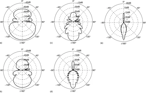
The far-field scattering results are shown in Fig.3and sum-marized in Table I. The radial quantity Hð Þh in the polar plots is the scattered power ratio, being the power in the scat-tered sound normalized to the power density in the incident wave, expressed in dB. It is calculated by
HðhÞ ¼
X1
m¼1
p2ffð^rh;mDtÞ
X1
m¼1
p2iðmDtÞ
: (20)
In all cases, the strongest scattering occurs at 180back toward the source and the characteristic7scattering nulls at690can also be observed. The main trends are that as the scattering volume is increased the scattering becomes stronger, more directional, and more selective in frequency. These three quan-tities are, respectively, quantified by the half-power (3 dB) lobe width W around 180, the backscattered power ratio Hð180Þand the Q-factor in frequency (the center frequency fmdivided by the half-power bandwidth). Figure4depicts the relationship between backscatter lobe width and scattering region outer radiusr0. The empirically fitted trend line follows
W ¼35 k=r0, showing that this backscatter directionality
is inversely proportional to the dimensions of the scattering volume. Figure 5 depicts the relationship between backscat-tered power ratio and scattering region volume Vscat and the trend line follows 0:213 V2
scat. The values ofH 180
ð Þwhich
are greater than 1 occur because the scattered power was nor-malized to the incident power density, and Vscat>1 m3. It is
interesting therefore that scattered power scales with V2 scat
instead of Vscat, since this implies the strength of the Bragg
backscatter mechanism is also proportional toVscat, though it
must saturate at some volume since it is not possible to scatter more energy than is incident. Data for Q-factor is more lim-ited. The data present in Table Iappears to be inversely pro-portional to r0, that is, a small scattering volume (including
only a few periods of the temperature fluctuations) gives broadband backscatter whereas a large scattering volume (including many periods of the temperature fluctuations) gives backscatter which is quite narrowband and highly dependent on the spacing of the temperature fluctuations. For the smallest scattering volumesr0¼0.15 m and 0.3 m,Qcould not be
cal-culated since the frequency content of the backscatter was lim-ited by the frequency content of the excitation, not by the frequency response of the backscattering process.
The second set of simulations examined the phase of the backscattered signal, since it has been established that this is important in remote sensing systems which utilize pulse compression.21 Here the standard values for r andr0 were
used and a number of simulations were run with small verti-cal shifts in the temperature profile defined by a random pa-rameter 0a2pwith
Tð Þ ¼r T0þwð Þr cos 4ð pfm^zr=cþaÞDT: (21)
factor). This is as expected since moving the temperature fluctuations amounts to changing the reflected path length and a delay (phase change in frequency) proportional to the increased path length will occur. This may seem like a trivial result; however, it will be drawn upon in the interpretation of the results in the next section.
B. Atmosphere with stochastic temperature fluctuations
In this section, an atmosphere with stochastic tempera-ture fluctuations is modeled and the far-field scattering compared to theoretical results. There is insufficient space here to adequately describe the subtleties and motivations of the atmospheric models used, and the interested reader
is directed toward Ref. 7 (Chap. 7) and Ref. 22
(Appendixes I and J), which provides a particularly accessi-ble explanation.
[image:8.612.56.558.44.365.2]It is assumed that the distribution of temperature fluctuations is homogeneous and isotropic, which is acceptable in a no-wind condition, and given by the Kolmogorov spectrum. Note that this differs from the study by Cheinetet al.13which used the von Karman spectrum. In three dimensions, the Kolmogorov spectral density as a function of wave numberkis given by
FIG. 3. Polar plots of far-field scattered power ratioHð Þh in dB versus angle for the “Bragg atmosphere” from smallest to largest scattering volume. (a)r0¼0.15 m, (b)
[image:8.612.314.559.530.720.2]r0¼0.3 m, (c)r0¼0.6 m, (d)r0¼1.2 m, (e)r0¼2.4 m.
TABLE I. Summary of far-field scattering by the “Bragg atmosphere.”r0is the outer radius of the scattering region,Vscatis the volume of the scattering
region,Wis the half-power lobe width,Hð180Þis the backscattered power ratio, andQis the Q-factor in frequency.
r0(m) r0=k Vscat(m3) W(deg) Hð180Þ(dB) Q
0.15 0.44 0.0096 64.1 44.5
-0.30 0.88 0.077 38.8 27.1
-0.6 1.8 0.61 20.4 10.1 5.55
1.2 3.5 4.90 10.2 5.77 11.0
2.4 7.1 39.2 5.13 21.1 21.8 FIG. 4. Backscattered lobe widthWversus scattering region outer radiusr0 for the “Bragg atmosphere.”
[image:8.612.53.297.664.746.2]Uð Þ ¼k C2T Cð8=3Þ
4p2 sinðp=3Þk
11=3: (22)
HereC2Tis the temperature structure parameter and on a summer day it typically takes values in the range 2 1010 m2=3
C2T=T
2
0 6 10
7m2=3 (Ref.7, Eq. 6.56). For the
simula-tions herein, a value toward the upper limit of this rangeC2T¼ 1:5 107T20 (larger amplitude temperature fluctuations) has
been used. Technically, this model is only valid within the range of characteristic eddy sizeLout1<k<L
1
in , termed the “inertial
subrange,” but this is not a problem as Lout is typically larger
than the inhomogeneous domainVandLinis smaller than the k-space grid spacing (and considered to be unimportant in acoustics22).
In what follows, it will be assumed that the temperature field (due to turbulence) is invariant during each SODAR pulse simulation; this amounts to a “frozen medium” approach and is valid where the rate of evolution of the temperature field is much lower than the speed of sound. Stochastic proper-ties are characterized by generating multiple random instances of the temperature field and averaging their responses. The individual instances of the temperature field are generated from sampled versions of Uð Þk by applying a random phase (i.e., spatial offset) to each coefficient of the discretized spec-trum and then applying a 3D inverse discrete Fourier trans-form; this is equivalent to the process described by Frehlich et al.23Note that for the Kolmogorov spectrum, the coefficient atk¼0 must be practically be omitted sinceUð Þ ¼ 10 . The smallest and largest wave number components reconstructed were therefore 2pdivided by the size of the modeling domain and 2pdivided by the grid spacing, respectively.
Figure 6 depicts a slice through a temperature offset profile calculated by this method, including windowing by wð Þr . As expected, there are rapidly varying features with small amplitude superimposed upon more slowly varying features with larger amplitude. The shape of the window wð Þr is also clearly visible. Temperature profile instances generated by this method will be referred to as “Kolmogorov atmospheres.”
Ostashev gives an analytical model for the scattering from stochastic atmospheres such as this in Sec. 7.1.3 of Ref.7. Re-writing it for temperature fluctuations only gives
r hð Þ ¼0:0041C
2
T T2 0
k1=3cos2h
sinðh=2Þ
ð Þ11=3: (23)
The quantityr hð Þis the scattering cross-section per unit vol-ume, and it is related to the scattered power ratio Hð Þh by Hð Þ h ð4pÞ2Vscatr hð Þ. Figure7shows the analytical model superimposed on a set of numerical results. The gray lines are the scattering from eight independent temperature profile realizations; these are stochastically generated so unsurpris-ingly they have quite irregular scattering patterns. The dark black line is the power average of these measurements and shows a much more regular pattern. The dashed line is the scattering predicted by analytical model, showing good agree-ment both in scattering pattern and amplitude despite the
[image:9.612.315.560.42.238.2]FIG. 6. (Color online) Slice through an instance of a temperature field (minus ambient) for an instance of a “Kolmogorov atmosphere.”
FIG. 5. Backscattered power ratioHð180Þvs scattering region volumeV scat for the “Bragg atmosphere.”
[image:9.612.52.297.44.235.2]relatively small number of simulation instances which are averaged (Cheinetet al.13use 200 instances in an equivalent calculation). A major discrepancy is however seen for the for-ward scattering aroundh¼0. Recall from Fig.2that a non-periodic temperature offset (i.e., with a spectrum that is large at smallk) produces a significant forward-scatter to account for the change in sound speed encountered as the wave passes through the domain. The classical model of large scattering angle for the Kolmogorov spectrum is an extreme example of this; it predicts infinite scattering ath¼0due to the infinite temperature offset implied by Uð Þ ¼ 10 . This behavior is not replicated in the numerical results because the infinite value ofUð Þ0 was omitted from the turbulence reconstruction on the grounds of being unphysical. In addition, the window-ing of the temperature fluctuations effectively imposes anLout
turbule size limit and significantly affects the forward scatter. A similar effect was seen for the von Karman spectrum by Cheinetet al.,13who go on to analyze the forward scattering case in much greater detail than is considered here.
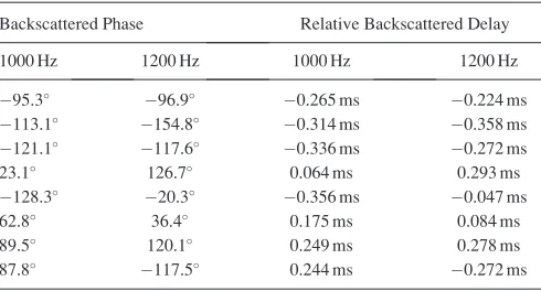
The result at the end of Sec. III A demonstrated that spatially offsetting periodic temperature fluctuations causes a related change of phase in the backscattered sound. Since instances of the Kolmogorov atmosphere may be thought of as a sum of such fluctuations spatially offset by a random amount, it follows that the phase of different frequency components in the backscattered sound will also be independently random. In addition, the backscattered phase for the same frequency will vary randomly for dif-ferent temperature field instances, for instance, during a SODAR measurement which is long with respect to the rate of evolution of the temperature field. Table II gives the phase of the signal backscattered from the eight simu-lated instances of the Kolmogorov atmosphere, both for fm¼1 kHz andfm¼1:2 kHz excitation; in the right hand columns, the corresponding relative delays have been cal-culated to permit easy comparison between the different frequency data. As expected there is no discernible rela-tionship between the backscattered phases at 1 kHz and 1.2 kHz; they appear to be independently random.
This result has implications for the design of pulse-compression algorithms for SODAR, since the matched filter-ing they utilize depends on a linear-phase time-invariant response. This means backscattered delay must be equal over
the operating bandwidth and time-invariant over each pulse sequence, and the discussion above and results in Table II
shows that this is not the case. As discussed in Ref.21, under these circumstances the benefits of the matched filtering are lost and the system performs no better than a non-coherent multi-frequency approach.
IV. DISCUSSION, CONCLUSIONS, AND FUTURE DIRECTIONS
This paper has described a numerical method for simu-lating far-field scattering from small regions of inhomogene-ous temperature fluctuations. The method combined an analytical incident sound model with ak-space model of the scattered sound close to the inhomogeneous region and a Near-to-Far-Field transformation to obtain far-field scatter-ing patterns. The algorithm was applied to two idealized test case atmospheres: one with periodic temperature fluctuations with height and one with stochastic temperature fluctuations given by the Kolmogorov spectrum, for which good agree-ment with classical results was seen. From that perspective, this paper may be thought of as an extension of some aspects of the work of Cheinet et al.13to three dimensions. The pa-per also aimed to draw conclusions about multi-frequency SODAR performance and to that end the phase of the back-scattered signals was analyzed. This suggested that stochas-tic atmospheres produce a randomized phase response which is independent with respect to frequency, suggesting atmos-pheric backscatter is an unsuitable target for matched-filter multi-frequency SODAR systems.
However, the model also has various limitations which require further discussion. One important aspect is that tur-bulent velocity fluctuations are omitted in this simulation (as they are in Sec. III B of Ref.13). This was justified by citing the classical result that only temperature fluctuations contrib-ute to the backscattered signal, but it would be desirable to properly test this assertion. With regard to the conclusions about randomized phase scattering from stochastic tempera-ture fluctuations, it is conceivable that velocity fluctuations may have an additional effect (they are, for example, known to cause a widening of the Doppler peak), but it seems far more likely that this would create further phase randomiza-tion rather than remove it. Considering the full propagarandomiza-tion path shown in Fig. 1, it is also clear that consideration has not been given to scattering processes between the SODAR and the scattering volume in either direction, and in a sto-chastic atmosphere these are also likely to be dispersive effects. It therefore seems reasonable to suppose that the sto-chastic features omitted from the model would further
com-promise the performance of the matched-filter post
processing in a multi-frequency SODAR, so the negative conclusions reached here are likely to be generalizable.
As regards the suitability of the method as a numerical testbed for a broader class of SODAR, it is clear that the omitted features described in the previous paragraph would be also desirable for this application. Stochastic velocity fluctuations due to turbulence could be incorporated within
the k-space model of the scattering region, though initial
[image:10.612.52.297.614.746.2]efforts suggest that this will be very computationally
TABLE II. Phase (and equivalent delay) of backscatter from the “Kolmogorov atmosphere.” Each row in the table presents the data from a different simulation instance.
Backscattered Phase Relative Backscattered Delay
1000 Hz 1200 Hz 1000 Hz 1200 Hz
95.3 96.9 0.265 ms 0.224 ms
113.1 154.8 0.314 ms 0.358 ms
121.1 117.6 0.336 ms 0.272 ms
23.1 126.7 0.064 ms 0.293 ms
128.3 20.3 0.356 ms 0.047 ms
62.8 36.4 0.175 ms 0.084 ms
89.5 120.1 0.249 ms 0.278 ms
87.8 117.5 0.244 ms 0.272 ms
expensive and probably require a GPGPU implementation. Another important extension would be to include tempera-ture and wind profiles through the atmosphere. It is antici-pated that these could be included by modifying only the incident and far-field parts of the model to account for the curvature those sound waves experience while propagating through the atmosphere, and that the k-space model of the scattering volume could be left largely unchanged (albeit perhaps cast into a moving coordinate system in the case of wind shear).
It would also be interesting to simulate the periodic tem-perature fluctuation scenario over many different cases over wider frequency bands, since it is essentially a building block of the stochastic atmosphere scenario. This may enable a bet-ter understanding of the scatbet-tering of sound by atmospheric turbulence and permit extraction of more trends, which could possibly even form the basis of an empirical model. However, the computation speed of the current code precludes this and a much faster implementation (e.g., GPGPU) would be neces-sary also to undertake this investigation.
The applicability of all these approaches, however, is built upon the validity of the Born approximation, which is essentially that forward scatter is negligible as a sound wave propagates through the atmosphere, meaning the backscatter from a small region may be calculated independently of the scattering from other regions. At first glance, Fig.7suggests that forward scattering is far from negligible, but as dis-cussed in Sec. III B, the forward scatter predicted there is predominately associated with slight changes in the speed of sound due to spatially large temperature fluctuations. Hence, it is likely to be non-dispersive and to not have a significant effect on SODAR measurements. Given an adequate compu-tational resource, it would be attractive to verify these assumptions by undertaking a small number of models of very large FDTD domains (themselves ideally verified against measurement), against which less computationally demanding algorithms (such as those proposed above) could ultimately be verified.
ACKNOWLEDGMENTS
This work was supported by the UK Engineering and
Physical Sciences Research Council [grant number
EP/G003734/1 “Advanced Signal Processing Methods
Applied to Acoustic Wind Profiling for Use in Wind Farm Assessment”]. The authors thank also Jonathan Sheaffer for his constructive feedback on an early version.
1S. G. Bradley,Atmospheric Acoustic Remote Sensing(Taylor and Francis
CRC Press, Florida, 2008), 328 pp.
2
S. G. Bradley, “Use of coded waveforms for SODAR systems,” Meteorol. Atmos. Phys.71, 15–23 (1999).
3
A. Nagaraju, A. Kamalakumari, and M. Purnachandra Rao, “Application of pulse compression techniques to monostatic doppler SODAR,” Glob. J. Res. Eng. 10, 37–40 (2010). Available online at http://www. engineeringresearch.org/index.php/GJRE/article/view/53/52.
4T. J. Cox, “Acoustic iridescence,” J. Acoust. Soc. Am.
129, 1165–1172 (2011).
5
V. I. Tatarski, Wave Propagation in a Turbulent Medium (Dover Publications Inc., New York, 1961), 285 pp.
6M. A. Kallistratova, “Backscattering and reflection of acoustic waves in
the stable atmospheric boundary layer,” IOP Conf. Ser. Earth Environ. Sci.1, 14 (2008).
7V. E. Ostashev,Acoustics in Moving Inhomogeneous Media(Spon Press,
London, 1997), 259 pp.
8
M. Legg, “Multi-frequency clutter-rejection algorithms for acoustic radars,” Masters thesis, The University of Auckland, Auckland, Australia, 2007.
9B. Piper, S. Bradley, and S. von Hunerbein, “Calibration method
princi-ples for monostatic sodars,” UPWIND Project Report (University of Salford, Manchester, UK, 2007).
10R. Blumrich and R. Heimann, “A linearized Eulerian sound propagation
model for studies of complex meteorological effects,” J. Acoust. Soc. Am.
112, 446–455 (2002).
11
V. E. Ostashev, D. K. Wilson, L. Liu, D. F. Aldridge, N. P. Symons, and D. Marlin, “Equations for finite-difference, time-domain simulation of sound propagation in moving inhomogeneous media and numerical implementation,” J. Acoust. Soc. Am.117, 503–517 (2005).
12
D. K. Wilson and L. Liu,Finite-Difference, Time-Domain Simulation of Sound Propagation in a Dynamic Atmosphere (US Army Corps of Engineers Engineer Research and Development Center, Hanover, NH, 2004).
13
S. Cheinet, L. Ehrhardt, D. Juve, and P. Blanc-Benon, “Unified modeling of turbulence effects on sound propagation,” J. Acoust. Soc. Am.132(4), 2198–2209 (2012).
14
R. J. Luebbers and M. Schneider, “A finite-difference time-domain near zone to far zone transformation,” IEEE Trans. Ant. Prop. 39, 429–433 (1991).
15A. Taflove and S. C. Hagness, Computational Electrodynamics—The Finite Difference Time-Domain Method (Artech House, Norwood, MA, 2005), 1038 pp.
16M. Tabei, T. D. Mast, and R. C. Waag, “Ak-space method for coupled
first-order acoustic propagation equations,” J. Acoust. Soc. Am. 111, 53–63 (2002).
17
M. Hornikx, R. Waxler, and J. Forssen, “The extended fourier pseudospec-tral time-domain method for atmospheric sound propagation,” J. Acoust. Soc. Am.128, 1632–1646 (2010).
18
B. E. Treeby and B. T. Cox, “k-Wave: MATLAB toolbox for the simu-lation and reconstruction of photoacoustic wave-fields,” J. Biomed. Opt. 15021314 (2010), http://www.k-wave.org/ (Last viewed 13 May 2013).
19
X. Yuan, D. Borup, J. Wiskin, M. Berggren, and S. A. Johnson, “Simulation of acoustic wave propagation in dispersive media with relaxa-tion losses by using FDTD method with PML absorbing boundary con-dition,” IEEE Trans. Ultrason. Ferroelectr. Freq. Control 46, 14–23 (1999).
20
A. D. Pierce, Acoustics: An Introduction to its Physical Principles and Applications(Acoustical Society of America, New York, 1989).
21
P. Kendrick and S. V. H€unerbein, “Pulse compression in SODAR,”16th International Symposium for the Advancement of Boundary-Layer Remote Sensing, Boulder, CO (2012).
22E. M. Salomons, Computational Atmospheric Acoustics (Kluwer
Academic Publisher, Boston, MA, 2001), 348 pp.
23