We a r r a t e-s t a t e i n t e r a c ti o n s
wi t hi n a m u l ti-c o m p o n e n t
s y s t e m : a s t u d y of a g e a r b o x
a c c e l e r a t e d lif e t e s ti n g p l a tfo r m
Ass af, R, Do, P, N e f ti-M e zi a ni, S a n d S c a rf, PA
h t t p :// dx. d oi.o r g / 1 0 . 1 1 7 7 / 1 7 4 8 0 0 6X 1 8 7 6 4 0 6 1
T i t l e
We a r r a t e-s t a t e in t e r a c ti o n s wi t hi n a m u l ti-c o m p o n e n t
s y s t e m : a s t u d y of a g e a r b o x a c c el e r a t e d lif e t e s ti n g
p l a tf o r m
A u t h o r s
As s af, R, Do, P, N ef ti-M e zi a ni, S a n d S c a rf, PA
Typ e
Ar ticl e
U RL
T hi s v e r si o n is a v ail a bl e a t :
h t t p :// u sir. s alfo r d . a c . u k /i d/ e p ri n t/ 4 5 1 6 8 /
P u b l i s h e d D a t e
2 0 1 8
U S IR is a d i gi t al c oll e c ti o n of t h e r e s e a r c h o u t p u t of t h e U n iv e r si ty of S alfo r d .
W h e r e c o p y ri g h t p e r m i t s , f ull t e x t m a t e r i al h el d i n t h e r e p o si t o r y is m a d e
f r e ely a v ail a bl e o nli n e a n d c a n b e r e a d , d o w nl o a d e d a n d c o pi e d fo r n o
n-c o m m e r n-ci al p r iv a t e s t u d y o r r e s e a r n-c h p u r p o s e s . Pl e a s e n-c h e n-c k t h e m a n u s n-c ri p t
fo r a n y f u r t h e r c o p y ri g h t r e s t r i c ti o n s .
multi-component system: a study of a
gearbox accelerated life testing platform
Reprints and permission:
sagepub.co.uk/journalsPermissions.nav DOI: 10.1177/ToBeAssigned www.sagepub.com/
Roy Assaf
1, Phuc Do
2, Samia Nefti-Meziani
1and Philip Scarf
3Abstract
The degradation process of complex multi-component systems is highly stochastic in nature. A major side effect of this complexity is that components of such systems may have unexpected reduced life and faults and failures that decrease the reliability of multi-component systems in industrial environments. In this work we provide maintenance practitioners with an explanation of the nature of some of these unpredictable events, namely the degradation interactions that take place between components. We begin by presenting a general wear model where the degradation process of a component may be dependent on the operating conditions, the component’s own state, and the state of the other components. We then present our methodology for extracting accurate health indicators from multi-component systems by means of a time-frequency domain analysis. Finally we present a multi-component system degradation analysis of experimental data generated by a gearbox accelerated life testing platform. In so doing, we demonstrate the importance of modelling the interactions between the system components by showing their effect on component lifetime reduction.
Keywords
Deterioration modelling, rate-state interaction, multi-component system, condition monitoring, gearbox, short-time fourier transform
1
Introduction
The increasing number of new manufacturing requirements is pushing original equipment manufacturers (OEM) to design more complex systems to fit the industrial needs. Such machines are becoming increasingly difficult to maintain (31; 32), especially due to their degradation processes becoming highly stochastic in nature. These degradation processes can limit the accuracy of diagnostics and remaining useful lifetime (RUL) predictions, leading to an increase in the number in unforeseen faults and failures and a reduction in the reliability of multi-component systems in industrial environments.
Consider for example a system with two components, an induction motor with a lifetime, say, up to 5 years that is coupled with bearings that have a lifetime that is but a fraction of this. In many multi-component systems like these, it is almost inevitable that after running the system for a long enough time, old worn out components will be coupled with new healthy components, and since old worn out components may potentially accelerate the degradation process of new components, it is in effect this old-new component coupling that affects the reliability of a system and leads to a system wearing out in an unforeseen accelerated fashion. Thus extracting correct health indicators and accounting for old-new component couplings in multi-component systems can play a crucial role in diagnosing the health state of a system.
Often however, the deterioration processes of components are assumed to be independent, see (7; 21; 29). But since real world systems are usually complex and include multiple interacting components, and that these inter-dependencies can potentially affect overall system availability, recently
condition based maintenance (CBM) research is showing a growing interest in multi-component systems (15).
In (19) The authors develop a CBM policy for systems with multiple failure modes. They consider that failures can occur before reaching a maintenance threshold, and that the failure rate of components can be influenced by the age of the system, the overall state of the system or both. This work however does not model the deterioration dependence between components and focuses mainly on the CBM policy rather than degradation modelling itself. In (13) the authors present a methodology for mixed signal separation of identical components using Independent component analysis (ICA), they specifically consider the case where there exists limiting constraints over sensor placement. They then use the separated signals as indicators of degradation severity for each of the components, and validate their approach via a numerical example using simulated degradation signals. Although this work is an essential step for modelling the degradation of such multi-component systems, it does not specifically model the
1School of Computing, Science & Engineering, Autonomous Systems
and Robotics Centre, University of Salford, Manchester, M5 4WT, UK
2CRAN (Research Centre for Automatic Control), University of Lorraine,
54506 Vandoeuvre-les-Nancy Cedex, France
3Salford Business School, University of Salford, Manchester, M5 4WT,
UK
Corresponding author:
Roy Assaf, School of Computing, Science & Engineering, Autonomous Systems and Robotics Centre, University of Salford, Manchester, M5 4WT, UK.
2 Journal Title XX(X)
deterioration dependence between components. In (6) the authors use stochastic differential equations to model the degradation between components. specifically they study how the degradation rate of one component can be influenced by the degradation state of other components with the aim of predicting residual lifetime of components. They then evaluate their approach using simulated data and compare it to a benchmark approach which assumed component degradation independence, finally showing the importance of capturing degradation dependencies between components. Although this work deals with deterioration dependence between components, it does not account for other interfering factors. In (18) the authors discuss what they refer to as the fault propagation phenomenon. This is described as the co-existence of inherent dependence and induced dependence when considering deterioration dependence between components. A continuous time Markov chain approach is developed to capture fault propagation characteristics. However this approach might suffer from state-space explosion problem, and does not consider other factors that may influence degradation and so does not describe the full underlying mechanism of system deterioration. In (24) and (9) the works consider state-rate degradation interactions. Both works study two component systems where they either consider a numerical simulation of a degradation process in (9), and perform degradation modelling for the particular case at hand in (24), They both then use the results for optimising the CBM policy. These works mainly deal with the optimisation of the CBM policy rather than developing a general degradation model for interdependent components.
Further to the works mentioned above, and considering the extensive body of literature on degradation modelling, see (30) and (29) for an overview, the literature shows that a component’s degradation process may depend on the system operating conditions such as the load on the system, vibration, humidity, temperature etc. see (4;8;27) and (10), and it is also shown that a system’s degradation process may depend on the system’s current state, see (26).
In this paper we aim to improve the accuracy of multi-component system diagnosis and prognostics by more accurately modelling the degradation process of such systems. We consider a practical generic model where the degradation process of a component may be dependent on the operating conditions, the component’s own state, and the state of the other components. We also provide a methodology for accurately extracting component health state information in a multi-component system and show the effect of degradation interactions between components, both through the use of numerical simulation and experimental data. The experimental data is obtained using the analysis of vibration arising from a gearbox accelerated life testing platform. Through this, we show the impact of old-new component couplings on the reduction of life expectancy of a new healthy component in a multi-component system.
The remainder of this paper is organised as follows: A general multi-component degradation model is presented in section 2 with a discussion on practical methods for fitting the proposed model parameters. In Section 3 we present our methodology which is used for extracting health indicators from a multi-component system with degradation
interactions. In section 4, we begin by presenting our experimental setting and scenarios of the gearbox accelerated life testing platform, we then show how we extract the state of the components from the data collected and show our analysis and results. Finally, section 5 concludes the paper.
2
Degradation modelling with rate-state
interactions
2.1
Degradation model and simulation
In this section, we will present our general degradation model for multi-component systems with degradation interactions as seen in (3).
Consider a multi-component system with n number of components. The degradation state of each component iis represented by an accumulation of wear over time which is assumed to be described by a scalar random variable Xi
t.
Componentifails if its degradation state reaches a threshold value Fi. If any of the components fail we consider the
system to have failed, and if a component is not operating for whatever reason, no change occurs to its degradation state unless a maintenance intervention is carried out.
We assume the evolution of the degradation state of componentiis represented by:
Xti+1=Xti+ ∆Xti (1)
where ∆Xi
t represents the degradation increment of
componentiduring one time step.
The degradation of a componentiat time steptmay depend on the operating conditions, the state of component i, and also the state of other components to a varying degree. Thus we suggest a general stationary model for the increment ∆Xi
t:
∆Xti= ∆Oti+ ∆Xtii+X
j6=i
∆Xtji (2)
where:
• ∆Oi
trepresents the degradation increment caused by
the operating conditions of component i during one time stept.∆Oi
tcan be specified as deterministic or
as a random variable.
• ∆Xii
t represents the degradation increment which is
intrinsic to i at time step t. In other words ∆Xtii
depends on the degradation state of component i at time step t. ∆Xtii can also be specified to be a
deterministic or random variable.
• P j6=i∆X
ji
t represents the sum of all degradation
increments which are caused by the interaction of componentiwith the other components of the system. The degradation interaction between a component i
and another componentj may be considered to be a deterministic or random variable.
We can now specify different variants of the proposed model:
Case 1: ∀ iin n,∆Oi
t>0,∆Xtii= 0 and∆X ji t = 0, in
this case there is neither an intrinsic nor an interaction effect, and so the proposed model is reduced to a model of homogeneous degradation behaviour of independent components as seen in (29).
Parameter Value
Component 1 Component 2 Component 3
Shapeα 4.944 4.35 5.193
[image:4.595.312.529.61.197.2]Scaleβ 3.919 1.09 2.257
Table 1. Simulation parameter values
Case 2: ∀ i inn,∆Oit>0,∆Xtii >0 and ∆Xtji= 0, in this case there is no degradation interaction between the components, and so the proposed model becomes a model describing non-homogeneous degradation behaviour as seen in (26).
Case 3: ∀ i in n, ∆Oi
t= 0, ∆Xtii = 0 and ∆X ji t >
0, in this case the components have degradation inter-dependencies only, and the proposed model corresponds to the degradation model that was introduced in (24).
Case 4: ∀ i in n, ∆Oi
t>0, ∆Xtii = 0 and ∆X ji t >0,
in this case the components have degradation inter-dependencies but no intrinsic degradation is present; this case then corresponds to the models presented in (6) and (9).
Case 5: ∀ i in n, ∆Oi
t>0, ∆Xtii >0 and ∆X ji t >
0, in this case the degradation processes of the components are dependent on the interaction between the components, the intrinsic degradation of the components and the operating conditions of the system.
It is assumed that if a component i reaches a specific threshold of degradation Fi it is then considered to have
failed.
For the purpose of illustrating the interactions that can influence the degradation process of components in a multi-component system, we will use Case 4 from the general deterioration model to create a numerical simulation of the degradation process of a 3 component system. Since the degradation of any component can only accumulate positively over time, we can then use a gamma process since it is widely used in degradation modelling as in (23; 29) to represent non-negative increments. And so for every componentiamong thencomponents of the system, the corresponding∆Oit follows a gamma distribution with distinct parameters, shapeαiand scaleβias shown in:
fαi,βi=
(βi)αi Γ(αi)x
αi−1exp−βi x (3)
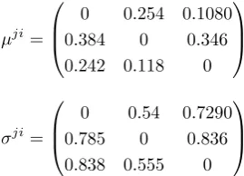
We can model inter-dependencies between components as presented in (9), and by extending from a two component system to a multi-component system we can now represent our general degradation model using the following:
∆Xti= ∆Oti+ ∆Xtii+X
j6=i
µji×(Xtj)σji (4)
whereµjiandσjiare non-negative real numbers which are used to quantify componentj’s influence on componenti.
Figure 1. Illustration of degradation evolution with rate-state interactions
And so by running a simulation using∆Oit’s gamma process
parameters given in Table1, along with theµjiandσjivalues as shown below, we can obtain degradation trajectories as seen in Fig.1.
µji=
0 0.254 0.1080
0.384 0 0.346
0.242 0.118 0
σji=
0 0.54 0.7290
0.785 0 0.836 0.838 0.555 0
From Fig.1, we can see the normal degradation trajectories of all 3 components from time step 1 till 40 since the system is considered to have started with all components having a healthy new state. We can now compare the normal deterioration trajectory of component 1 with it’s accelerated deterioration after being replaced at time step 42 and being coupled with the other two worn out components. We can clearly see two phases of accelerated degradation after component 1 has been replaced with a new component, a highly accelerated degradation from time step 42 till 48, then a somewhat less accelerated degradation from time step 49 till 56. The first highly accelerated degradation is due to the fact that a new component 1 was interacting with a worn out component 2 and a severely worn out component 3 that was above 75% deteriorated; subsequently, the less accelerated degradation is a result of the replacement of component 3 with a new component at time step 49.
This old-new component coupling is clearly influencing the lifetimes of the components after being replaced with new ones. This kind of interaction can lead to accelerated degradation of the components and the system as a whole, thus resulting in unexpected faults and failures. The result of this old-new component interaction will be analysed using experimental results described in section4of this paper.
2.2
Parameter identification
[image:4.595.355.490.310.407.2]4 Journal Title XX(X)
There exists an extensive body of literature on the topic of parameter identification see for example (1;12;20).
In practice, if the degradation model is not too complex, we can fit the model parameters using Maximum likelihood estimation. However if the model is too complex or if we are collecting online observation on the health condition of the components and would like to achieve real time prognostics, we suggest to use sequential Monte Carlo methods, specifically the particle filter (PF) which is a very popular approach for parameter estimation (11). This allows for an online numerical estimation of the parameter values by means of a recursive Bayesian inference approach. The posterior distribution of the model parameters can be then obtained using a number of particles and their corresponding weights. This method is very flexible and can be used for non-linear models where the noise is not necessarily Gaussian. Such an approach has been successfully used in the field of prognostics for model parameter estimation as seen in the works of (17;22;33).
Say we would like to estimate the parameters of a degradation model that corresponds toCase 4. Let’s assume the operational effect is stochastic and follows a gamma distribution∆Oi
t is i.i.d. Γ(αi, βi), and that we have two
interacting components where the interaction is modeled as presented in (9). Then the deterioration model can be rewritten as:
Xti+1=Xti+ Γ(αi, βi) +µji×(X j t)σ
ji
(5)
In this case there exists two sets of parameters Θ1 and Θ2. Where Θ1= (α1, β1, µ21, σ21, ) and Θ2=
(α2, β2, µ12, σ12, )with ,representing the variance of the
observation noise which can be assumed to be Gaussian. For each set of parameters we generate a specificnnumber of particles, each having 5 parameter values selected at random from a prior distribution. We then generate a prediction of the next health conditionx˜it+1fori= 1 :n. After observing the next health conditionxit+1we can calculate the importance
weight of each particle by computing the likelihood of that observation given the predicted values of each particle
p(xi
t+1|x˜it+1). We then normalise the weights and perform
bootstrap sampling i.e. we re-sample with replacement n
particles from the previous set of particles. For more in depth information about PF we suggest reading (11).
The following section details our methodology for acquiring component health state data from real multi-component systems.
3
A methodology for component state
extraction
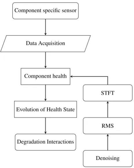
The methodology for state indicator extraction is presented as a flowchart in Fig.2. As shown, we start by acquiring data from sensors, specifically vibration data, since it has been extensively studied and successfully used for the purposes of diagnosing industrial rotating machinery, mainly for components such as gears (16), bearings (2; 28) and induction motors (5).
After acquiring data from multi-component systems, a major challenge for modelling existing inter-dependencies is the complex nature of the signals acquired, where each signal may represent a mixture of the signals of all components
Component specific sensor
Data Acquisition
Component health
STFT
RMS
Denoising Evolution of Health State
[image:5.595.309.541.51.341.2]Degradation Interactions
Figure 2. Methodology for extracting components’ state indicators and interactions in a multi-component system
at once, but to varying degrees. So an accurate way of acquiring component specific degradation state information from multi-component systems is to consider time-frequency domain analysis of the acquired signals. To motivate our use of time-frequency domain analysis over the other common waveform data analysis approaches, namely time-domain analysis and frequency domain analysis (14), we will briefly overview them and show their advantages and shortcomings in a multi-component system diagnosis scenario.
Time domain analysis is applied to the signals acquired in their time waveform. Common time domain analyses will mainly include descriptive statistics of the signal such as the mean value, standard deviation, root mean square, crest factor, skewness, kurtosis, etc. And so although this approach is typically computationally more efficient than other techniques, due to gathering statistics directly from the time waveform signal, this kind of analysis will rarely be able to differentiate which component is responsible for which changes in the signals, and will serve poorly when trying to model the degradation interdependence of components.
Another approach is frequency domain analysis. This is applied to the frequency domain transform of the acquired time waveform signals, usually by applying a discrete Fourier transform (DFT) on the signal, or other more computationally efficient variants for computing DFT, algorithms such as the fast Fourier transform (FFT). In the frequency domain, one can clearly see the ratio of influence of the different frequency bands on the time waveform signal, and although this can be related directly to the physical systems associated with the different frequencies, this approach on its own will fail to show us the evolution of these ratios with time, again an essential part would be missing for modelling inter-dependencies between components.
Algorithm 1:Outlier Removal algorithm
wrepresents the window length;
input :RMS signalSig, a row matrix of size
m×w
output:RMS signal with no outliers
fori←1tomdo
med←ComputeMedian(Sig(i)); mad←ComputeMAD(Sig(i));
forj←1towdo
ifSig(i, j)<(med−mad)or Sig(i, j)> (med+mad)then
Sig(i, j) =X∼ N(med, mad)
end end end
Finally we have time-frequency domain analysis; tech-niques such as the Short Time Fourier Transform (STFT) that allow for the analysis to be performed in both the time and frequency domains, isolating the frequency components of interest all while representing their evolution with time. This gives time-frequency domain analysis an advantage over the two previously mentioned approaches since it allows the han-dling of non-stationary waveform signals. Consequently, we will use a time-frequency domain analysis when performing diagnosis on multi-component systems.
Therefore, in order to extract the health states of components accurately, we apply the STFT over the time-waveform data as shown in:
ST F Ts(t, ω) =
+∞
Z
−∞
h(τ−t)s(t) exp−jωtdt (6)
This will allow us to isolate frequencies of interest all while showing the evolution of the energy through time. Then we can compute the root mean square (RMS) over a the frequency band of interest, as given by:
XRM S = v u u t
1 N
N X
i=1
x(i)2 (7)
to estimate how the magnitude of the frequency band of interest evolves in time. In this way, we can study a time series signal that describes the evolution of the condition of components over time.
[image:6.595.305.545.53.295.2]Finally since we are dealing with physical systems, where clean data are not often encountered, data cleaning of the acquired time series should be performed. An example of an outlier removal algorithm is detailed in Algorithm1. First we would need to specify a window of data points based on the operating profile of the system is specified. Then the median value or geometric mean of the data and the median absolute deviation (MAD) are computed. Then values that exceed the median plus or minus the MAD value are filtered by replacing them with a random variable sampled asX ∼ N(med, mad), thus preserving as much as possible the true nature of the signal.
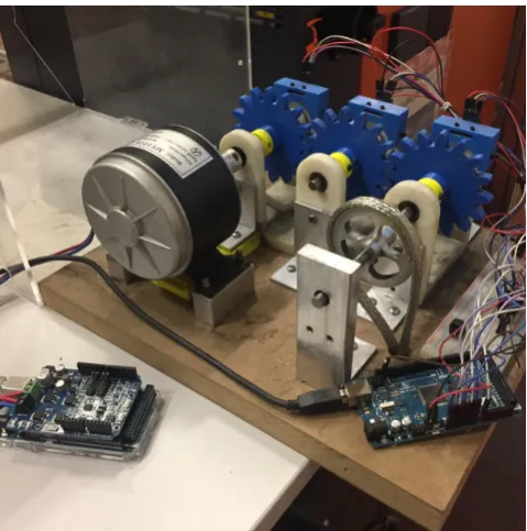
Figure 3. Gearbox accelerated life testing platform
4
Case Study
In an industrial setting, gearboxes are present in virtually any mechanical system, playing the essential role of torque and speed conversion, and unforeseen faults can lead to lowered machine up time and less plant efficiency. A gearbox is a good example of a system with multiple components. Therefore with the aim of collecting data on multi-component interactions we carried out our experiments on a gearbox accelerated life testing platform as shown in Fig.3.
6 Journal Title XX(X)
Figure 4. Raw accelerometer data from Gears 1 and 2, represented in Gs.
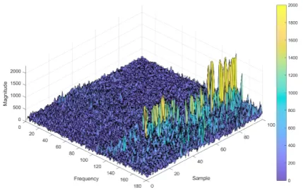
Figure 5. Visual representation of the spectrum of frequencies of Gear 1 in Run 1 varying with time
sensors collect data on three axis and have a full sensing range of±3Gs. To avoid distortion of vibration signals, these accelerometers are each mounted over the centerline of the shaft supporting bearing. We do this by fixing these sensors using hex socket screws to a 3D printed housing that lies on top of the frame of the gearbox.
The experimental runs of the gearbox were designed for accelerated life testing, thus achieving failure in a shorter amount of time than it would usually take under normal operating conditions. These runs are an alternating sequence of two types of cycles; the first cycle is a low speed low load cycle, referred to as LSLL; and the second type is a high speed high load cycle, referred to as HSHL. The vibration measurements used in this study were collected in the LSLL cycles in order to improve the signal to noise ratio (SNR). We computed the SNR to be on average 10.6dB using the following:
SN R=Psignal Pnoise
(8)
SN RdB = 10 log10(SN R) (9)
4.1
Experimental scenarios
[image:7.595.67.274.61.203.2]To demonstrate the degradation interaction that takes place between an old worn out component and a new healthy component, we will consider only two gears in the system, gear 1 and gear 2 referred to as G1 and G2 respectively.
Figure 6. Degradation time series of gears 1 and 2. In blue the first acquired time series signal, and in red an overlay after
applying the outlier removal algorithm.
The Gearbox platform was run three times in the following manner:
Run 1: the first run consisted of a new G1 and a new G2. The gearbox was run alternating between HSHL and LSLL until high levels of vibration were observed in the gearbox at which point the experimental run was terminated.
Run 2: After the first run, G1 was replaced with a new gear, while G2 remained unchanged, so the second run consisted of a new G1 and a worn out G2. The gearbox was ran alternating between the two cycles until high vibration was observed; on this run high system vibration occurred in a shorter amount of time, and after terminating the run, G2 showed more severe damage on it’s teeth surface than that observed after the termination of run 1.
Run 3: In the third run, G1 was replaced with a new gear, while G2 remained unchanged, so we find ourselves with a similar condition scenario as in run 2, this time however with a more worn out G2. The gearbox ran alternating between the two cycles until high vibration was observed. This run lasted an even shorter amount of time than in run 2, and so the run was terminated earlier than in run 1 and run 2.
Vibration data were collected from the accelerometers in all three runs, and treated using the methodology discussed in section3.
4.2
Component state extraction
A sample of duration 2 seconds of reading from the accelerometers of gears 1 and 2 can be seen in Fig.4. This raw time waveform vibration data were then turned into time-frequency domain data using STFT resulting in a spectrogram as shown in Fig.5. Now using the number of teeth of the gearsN = 16, we computed the gear meshing frequency to be around 120Hz using the following formula:
fmesh=RP M×N (10)
Now we use a frequency band of 5Hz, dynamically allocated over the spectrogram due to changes in the meshing
[image:7.595.61.276.260.395.2]LSLL Cycle Number
Run Gear 1 2 3 4 5 6 7 8 9 10
1 1 5.1 4.83 4.58 6.69 4.38 5.03 3.42 9.04 12.94 11.32
1 2 6.26 5.05 5.81 6.48 4.64 7.12 5.03 10.51 9.92 10.95
2 1 5.82 4.58 6.32 5.71 10.82 9.28
2 2 8.39 8.35 8.72 8.56 11.1 10.8
3 1 6.62 6.38 8.94 10.3
[image:8.595.110.491.58.184.2]3 2 10.84 8.85 10.34 11.95
Table 2. Average Gear meshing frequency magnitude for each LSLL cycle for both gears in all there runs.
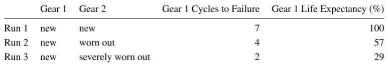
Gear 1 Gear 2 Gear 1 Cycles to Failure Gear 1 Life Expectancy (%)
Run 1 new new 7 100
Run 2 new worn out 4 57
Run 3 new severely worn out 2 29
Table 3. Effect of deterioration on component interactions
frequency caused by small variations in the rotational speed of the system, to accurately capture the magnitude of the gear meshing frequency in time. We then computed the RMS value for each time step, which results in the degredation time series shown in Fig.6, where the experimental runs are separated by the dashed red vertical lines, the silver dashed vertical lines represent the start of a new data collection cycle, i.e. an LSLL cycle, and noting that a) between every 2 LSLL cycles there exists an HSHL cycle, and b) The HSHL vibration data were not used and is thus not represented in this figure.
4.3
Results
Based on the experimental runs, the vibration signals emitted and the wear observed on the surface of the teeth of the gears, we can set the failure threshold asF = 8. Therefore when a gear meshing frequency magnitude is greater or equal to 8, as can be seen in Fig.6, the system is considered to have failed, or severely degraded in the sense that the platform is no longer operable in a normal condition.
Now in order to indicate the degradation interactions between the two gears, we compute the average of each LSLL cycle and display the obtained values in Table2. Note that here the average vibration doesn’t necessarily increase at every LSLL, this small fluctuation is due to the change between HSHL and LSLL which can distort the signal acquired by the accelerometers when capturing vibration data. However, we can already see that there is a general trend of increase in vibration with the increase in LSLL cycle count which indicates the degradation of the Gears.
The degradation interactions can already be detected when looking at Table 2, however for a more clear view of the interactions that are taking place, we can look at Table 3
which indicates the time to failure of the components, and there we can clearly see the accelerated degradation of the Gears that is due to their interaction.
As shown from Table 2 in Run 1, it takes seven cycles to reach the G1 failure limit when both gears are new. We can consider this as normal degradation behaviour of
the components and so we can say that in this case, the life expectancy of a component when coupled with a new component is 100%. Now looking at Run 2, we see that it takes four cycles to reach the G1 failure limit when G1 is new and G2 is worn out. Thus compared to Run 1, where both gears were new, we see that having a new component coupled with a worn out component would lead to accelerated wear of the new component and so the life expectancy is reduced to only 57%, in this case, in comparison with normal degradation of the components. Finally in Run 3 we see that it takes only two cycles until G1 reaches its failure limit when G1 is new and G2 is severely worn out. This means that in comparison to normal degradation behaviour G1 had, in this case, a life expectancy of 29% relative to that under normal degradation. This is clearly shown in summary in Table3.
Such results demonstrate the importance of modelling in the state of other components when performing diagnosis or prognosis on a multi-component system. For if we were to replace a specific component in the system with a new one, ignoring the accelerated degradation effect that would result from it being coupled with a now worn out component, there would arise unexpected failures and faults, caused by the reduced lifetime of the new installed components that were not operating under what would be considered to be normal conditions.
5
Conclusions
[image:8.595.104.491.213.279.2]8 Journal Title XX(X)
the system health by showing the degradation interaction that results when the components of a system are in different health states. We validate this approach and demonstrate our analysis on experimental data collected from a gearbox accelerated life testing platform. Here we show that when a new gear is coupled with a worn out gear, the life expectancy of the new gear may be reduced to 29% of that of a new gear coupled with another new gear. Through this work we show the importance of accounting for the state of other components when diagnosing the health of a system as a whole, since old-new component couplings can ultimately lead to accelerated wear out of the system.
Our future work will focus on the fitting of the proposed degradation model to acquired experimental data, along with providing a comparative study of state of the art machine learning algorithms, and assessment of their prognostic accuracy when different health features are extracted from multi-component systems.
Acknowledgements
The research leading to these results has received funding from the People Programme (Marie Curie Actions) of the European Union’s 7th Framework Programme FP7/2007-2013/ under REA grant agreement number 608022.
References
[1] Dawn An, Nam H Kim, and Joo-Ho Choi. Practical options for selecting data-driven or physics-based prognostics algorithms with reviews. Reliability Engineering & System Safety, 133:223–236, 2015.
[2] Xueli An and Dongxiang Jiang. Bearing fault diagnosis of wind turbine based on intrinsic time-scale decomposition frequency spectrum. Proceedings of the Institution of Mechanical Engineers, Part O: Journal of Risk and Reliability, 228(6):558–566, 2014.
[3] Roy Assaf, Phuc Do, Phil Scarf, and Samia Nefti-Meziani. Wear rate-state interaction modelling for a multi-component system: Models and an experimental platform. IFAC-PapersOnLine, 49(28):232–237, 2016.
[4] Piero Baraldi, Michele Compare, Antoine Despujols, and Enrico Zio. Modelling the effects of maintenance on the degradation of a water-feeding turbo-pump of a nuclear power plant.Proceedings of the Institution of Mechanical Engineers, Part O: Journal of Risk and Reliability, 225(2):169–183, 2011.
[5] M El Hachemi Benbouzid. A review of induction motors signature analysis as a medium for faults detection. IEEE transactions on industrial electronics, 47(5):984–993, 2000. [6] Linkan Bian and Nagi Gebraeel. Stochastic framework for
partially degradation systems with continuous component degradation-rate-interactions. Naval Research Logistics (NRL), 61(4):286–303, 2014.
[7] Keomany Bouvard, Samuel Artus, Christophe B´erenguer, and Vincent Cocquempot. Condition-based dynamic maintenance operations planning & grouping. application to commercial heavy vehicles. Reliability Engineering & System Safety, 96(6):601–610, 2011.
[8] Estelle Deloux, Bruno Castanier, and Christophe B´erenguer. Predictive maintenance policy for a gradually deteriorating
system subject to stress. Reliability Engineering & System Safety, 94(2):418–431, 2009.
[9] Phuc Do, Phil Scarf, and Benoi Iung. Condition-based maintenance for a two-component system with dependencies. IFAC-PapersOnLine, 48(21):946–951, 2015.
[10] Phuc Do, Alexandre Voisin, Eric Levrat, and Benoit Iung. A proactive condition-based maintenance strategy with both perfect and imperfect maintenance actions. Reliability Engineering & System Safety, 133:22–32, 2015.
[11] Arnaud Doucet and Adam M Johansen. A tutorial on particle filtering and smoothing: Fifteen years later. Handbook of nonlinear filtering, 12(656-704):3, 2009.
[12] Nagi Gebraeel and Jing Pan. Prognostic degradation models for computing and updating residual life distributions in a time-varying environment.IEEE Transactions on Reliability, 57(4):539–550, 2008.
[13] Li Hao, Nagi Gebraeel, and Jianjun Shi. Simultaneous signal separation and prognostics of multi-component systems: the case of identical components. IIE Transactions, 47(5):487– 504, 2015.
[14] Andrew KS Jardine, Daming Lin, and Dragan Banjevic. A review on machinery diagnostics and prognostics implement-ing condition-based maintenance. Mechanical systems and signal processing, 20(7):1483–1510, 2006.
[15] Minou CA Olde Keizer, Simme Douwe P Flapper, and Ruud H Teunter. Condition-based maintenance policies for systems with multiple dependent components: A review. European Journal of Operational Research, 2017.
[16] Mitchell Lebold, Katherine McClintic, Robert Campbell, Carl Byington, and Kenneth Maynard. Review of vibration analysis methods for gearbox diagnostics and prognostics. In Proceedings of the 54th meeting of the society for machinery failure prevention technology, volume 634, page 16, 2000. [17] Ping Li, Roger Goodall, and Visakan Kadirkamanathan.
Parameter estimation of railway vehicle dynamic model using rao-blackwellised particle filter. InEuropean Control Conference (ECC), 2003, pages 2384–2389. IEEE, 2003. [18] Zhenglin Liang, Ajith Kumar Parlikad, Rengarajan
Srini-vasan, and Nipat Rasmekomen. On fault propagation in deterioration of multi-component systems. Reliability Engi-neering & System Safety, 162:72–80, 2017.
[19] Xiao Liu, Jingrui Li, Khalifa N Al-Khalifa, Abdelmagid S Hamouda, David W Coit, and Elsayed A Elsayed. Condition-based maintenance for continuously monitored degrading systems with multiple failure modes. IIE Transactions, 45(4):422–435, 2013.
[20] Ariane Lorton, Mitra Fouladirad, and Antoine Grall. A methodology for probabilistic model-based prognosis. European Journal of Operational Research, 225(3):443–454, 2013.
[21] Kim-Anh Nguyen, Phuc Do, and Antoine Grall. Condition-based maintenance for multi-component systems using importance measure and predictive information.International Journal of Systems Science: Operations & Logistics, 1(4):228–245, 2014.
[22] Marcos E Orchard and George J Vachtsevanos. A particle-filtering approach for on-line fault diagnosis and failure prognosis. Transactions of the Institute of Measurement and Control, 31(3-4):221–246, 2009.
[23] Zhengqiang Pan and Narayanaswamy Balakrishnan. Reliabil-ity modeling of degradation of products with multiple perfor-mance characteristics based on gamma processes. Reliability Engineering & System Safety, 96(8):949–957, 2011. [24] Nipat Rasmekomen and Ajith Kumar Parlikad.
Condition-based maintenance of multi-component systems with degra-dation state-rate interactions. Reliability Engineering & System Safety, 148:1–10, 2016.
[25] Abdulrahman S Sait and Yahya I Sharaf-Eldeen. A review of gearbox condition monitoring based on vibration analysis techniques diagnostics and prognostics. Rotating Machinery, Structural Health Monitoring, Shock and Vibration, Volume 5, pages 307–324, 2011.
[26] Xiao-Sheng Si, Wenbin Wang, Chang-Hua Hu, Dong-Hua Zhou, and Michael G Pecht. Remaining useful life estimation based on a nonlinear diffusion degradation process. IEEE Transactions on Reliability, 61(1):50–67, 2012.
[27] Sanling Song, David W Coit, and Qianmei Feng. Reliability for systems of degrading components with distinct component shock sets.Reliability Engineering & System Safety, 132:115– 124, 2014.
[28] N Tandon and A Choudhury. A review of vibration and acoustic measurement methods for the detection of defects in rolling element bearings.Tribology international, 32(8):469– 480, 1999.
[29] JM Van Noortwijk. A survey of the application of gamma processes in maintenance. Reliability Engineering & System Safety, 94(1):2–21, 2009.
[30] Hongzhou Wang. A survey of maintenance policies of deteriorating systems. European journal of operational research, 139(3):469–489, 2002.
[31] Shen Yin, Steven X Ding, and Donghua Zhou. Diagnosis and prognosis for complicated industrial systemspart i. IEEE Transactions on Industrial Electronics, 63(4):2501–2505, 2016.
[32] Shen Yin, Steven X Ding, and Donghua Zhou. Diagnosis and prognosis for complicated industrial systemspart ii.IEEE Transactions on Industrial Electronics, 63(5):3201–3204, 2016.