Essays on Alternative Perspectives on Cross Border B2B Trust and Commitment

(1)

Georgia State University

ScholarWorks @ Georgia State University

Economics Dissertations Department of Economics

12-11-2018

Essays on Medical Marijuana Laws, Health

Insurance and Health Care Utilization

Pelin Ozluk

Follow this and additional works at:https://scholarworks.gsu.edu/econ_diss

This Dissertation is brought to you for free and open access by the Department of Economics at ScholarWorks @ Georgia State University. It has been

Recommended Citation

Ozluk, Pelin, "Essays on Medical Marijuana Laws, Health Insurance and Health Care Utilization." Dissertation, Georgia State University, 2018.

(2)

ABSTRACT

ESSAYS ON MEDICAL MARIJUANA LAWS, HEALTH INSURANCE AND HEALTH

CARE UTILIZATION

BY

PELIN ¨OZL ¨UK

AUGUST 2018

Committee Chair: Charles Courtemanche

Major Department: Economics

National Health Expenditures Accounts estimates that U.S health care spending grew

4.3 percent from the previous year to reach $3.3 trillion, or $10,338 per person in 2016.

The overall share of gross domestic product (GDP) related to health care spending was 17.9

percent in 2016, up from 17.7 percent in 2015. Moreover, increased use of opioid prescriptions

led to excessive use and abuse of these drugs, resulting in nationwide “opioid epidemic”. This

dissertation examines how different policy interventions contributed to the rise in health care

utilization and prescribed opioids in U.S.

The first chapter examines how medical marijuana laws changed utilization of prescription

drugs with a special emphasis on prescribed opioids. More than half of the US population

lives in a state that has adopted medical marijuana laws (MMLs). Studies show that most

medical marijuana patients use marijuana for managing their pain with the overwhelming

majority of them preferring it to opioids. Despite ongoing pro-marijuana policies and the

growing trend of public acceptance, the evidence on how people change their prescription

use due to the availability of marijuana as an alternative treatment is limited. Using the

variations across state MMLs between 1996 and 2014 of Medical Expenditure Panel Survey

(3)

focus on opioids. I find that MMLs lead to a $2.47 decrease in per person prescribed opioid

spending among young adults (ages 18-39) over a year. Most of this decrease results from

the intensive margin of use and MML states that allow home cultivation experience even

larger decreases. Furthermore, the decreasing effects are persistent over time and they get

stronger following the years of implementation. MMLs also decrease the number of opioid

pill use among young adults. I do not find any discernible impact on older populations'

opioid utilization. I then investigate the effects on other prescriptions for which marijuana

can be a potential substitute and find the allowance of dispensaries is generally associated

with decreases, although the effects depend on the type of MML, the margin of use and age.

The second chapter examines how universal insurance coverage affects health care

utiliza-tion drawing evidence from the health reform of Massachusetts in 2006. This law reformed

insurance markets, mandated that all residents in the state would be required to take up

health insurance, and provided subsidies for lower-income individuals to purchase it. Using

data from MEPS between 2000 and 2015, I provide evidence that the Massachusetts health

care reform increased counts of hospital and office-based medical provider visits significantly.

The results were robust to using alternative control groups and different functional form

as-sumptions. I find the reform's effects grew over time, reaching its maximum after 2010. The

reform also increased health care expenditures and probability of health care service use

significantly. Finally, I use the reform to instrument for health insurance and estimate large

impacts of insurance on health care utilization.

The third chapter examines the impact of the Affordable Care Act on health care

uti-lization. The Affordable Care Act (ACA) aimed to achieve nearly universal health insurance

coverage in the United States through a combination of regulations, mandates, subsidies,

exchanges, and Medicaid expansions. We use data from the Medical Expenditure Panel

Survey (MEPS) to investigate the impacts of the ACA on the health care utilization and

(4)

identifies the effects of the ACA's expansions of private and Medicaid coverage by leveraging

variation in states'Medicaid expansion decisions and individuals'pre-ACA insurance status.

Intuitively, impacts of the ACA's insurance expansions should be concentrated among those

who lacked insurance prior to the law, and such individuals are more likely to be affected

in states that participated in the Medicaid expansion. Similar methods have been used to

study the ACA's effects on outcomes such as health insurance coverage, access to care, risky

health behaviors, and self-assessed health. However, they have not been previously used to

investigate impacts on health care spending. Theoretically, the net effect on spending is

ambiguous. On one hand, insurance lowers the effective price of care, which should increase

utilization across-the-board. On the other hand, insurance improves access to primary and

preventive care, which could potentially reduce use of expensive emergency services. The

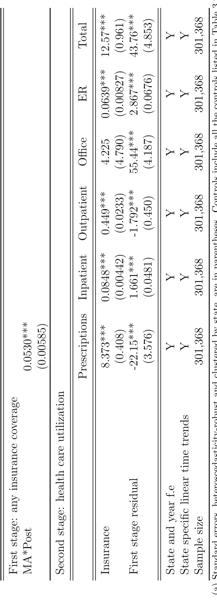
results suggest that the ACA increased health care utilization in some dimensions –

in-cluding counts of inpatient hospital visits, medical-provider office visits and total counts of

prescription fills, inpatient, outpatient, medical-provider office and ER visits combined on

its first year. However, these increases in health care utilization in counts were not observed

in ACA's second year. We also found that the ACA increased coverage and led to significant

gains in both expansion and non-expansion states consistent with what has been found by

prior studies. This significant gain in insurance was not limited to ACA's first year but it

(5)

ESSAYS ON MEDICAL MARIJUANA LAWS, HEALTH INSURANCE AND HEALTH

CARE UTILIZATION

BY

PELIN ¨OZL ¨UK

A Dissertation Submitted in Partial Fulfillment

of the Requirements for the Degree

of

Doctor of Philosophy

in the

Andrew Young School of Policy Studies of

Georgia State University

GEORGIA STATE UNIVERSITY

(6)

Copyright by Pelin ¨Ozl¨uk

(7)

ACCEPTANCE

This dissertation was prepared under the direction of Pelin ¨Ozl¨uk’s Dissertation Committee. It has been approved and accepted by all members of that committee, and it has been accepted in partial fulfillment of the requirements for the degree of Doctor of Philosophy in Economics in the Andrew Young School of Policy Studies of Georgia State University.

Dissertation Chair: Charles Courtemanche

Committee: James Marton

Shiferaw Gurmu Jason Hockenberry

Electronic Version Approved:

Sally Wallace, Dean

Andrew Young School of Policy Studies Georgia State University

(8)

DEDICATION

(9)

ACKNOWLEDGMENTS

I would like to express my deepest appreciation to my advisor, Chuck Courtemanche for

guiding and supporting me over the years. Without his guidance this dissertation would not

have been possible. He has set an excellent example of a mentor, and role model for me. I

would also express my gratitude to my dissertation committee members Jim Marton, Shif

Gurmu and Jason Hockenberry for all of their guidance through this process; their discussion,

ideas, and feedback have been invaluable. I would also like to thank Tom Mroz for always

being available to discuss and guide my research, and Garth Heutel for his support.

I am extremely grateful to my mom, Vicdan Din¸c for her endless love, support and

protection. I would not have been who I am without her by my side. I am deeply grateful to

my sister, Ekin ¨Ozl¨uk for being my best friend and my guide in life. I am incredibly lucky

to have her as my sister. I would also extend my deepest gratitude to my brother in law

Jason Neymeyer who has been an excellent role model and my support system for me over

the years. I also owe many thanks to my father Kenan ¨Ozl¨uk for always being on my side.

I would like to extend my thanks to my best friends in life, Lale Se¸cginli and Aylin Kertik

for their endless love and friendship. I am very grateful to have met you earlier in life so I

could grow with you. I am deeply thankful to all the other great friends I have made in the

program. They have been incredibly supportive and made my experience at Georgia State

fun. I want to specifically thank Rhita Simorangkir for her genuine friendship.

Last but not least, I would like to express my gratitude to Kuzu, Koko, Buck and Teddy

(10)

List of Figures

1.1 Distribution of opioid expenditures - Ages 18+ . . . 67

1.2 Results from event study analyses on opioid expenditures . . . 68

2.1 Changes in Health Care Service Use Counts 2000 to 2015 . . . 69

(13)

List of Tables

1.1 Medical marijuana laws and provisions by state, 1996-2014 . . . 70

1.2 Summary statistics for outcome variables . . . 71

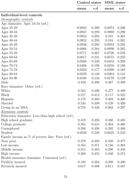
1.3 Summary statistics for control variables . . . 72

1.4 Ages 18-39 - Average marginal effects on opioid spending . . . 73

1.5 Ages 40-64 - Average marginal effects on opioid spending . . . 74

1.6 Ages 65+ - Average marginal effects on opioid spending . . . 74

1.7 Effects of different policy combinations on opioid expenditures . . . 75

1.8 Average marginal effects on opioid pills . . . 75

1.9 Other medicines Ages 18-39 . . . 76

1.10 Other medicines Ages 40-64 . . . 77

1.11 Other medicines Ages 65+ . . . 78

1.12 Placebo Test Ages 18-39 . . . 79

1.13 Placebo Test Ages 40-64 . . . 80

1.14 Placebo Test Ages 65+ . . . 81

2.1 Means of control variables . . . 82

2.2 Means of outcome variables . . . 83

2.3 Effects of the reform on health care utilization of counts: Average marginal effects from negative binomial . . . 84

2.4 Effects of the reform on health care utilization of counts: Average marginal effects from hurdle model . . . 84

2.5 Effects of the reform on health care utilization on spending: Average marginal effects from two-part model . . . 85

2.6 Effects of the reform on health care utilization on the extensive margin: Av-erage marginal effects from probit . . . 85

2.7 Effects of the reform on health care utilization on the intensive margin: Av-erage marginal effects from GLM . . . 86

2.8 Match on pretreatment levels: Average marginal effects from negative binomial 86 2.9 Match on pretreatment trends: Average marginal effects from negative binomial 87 2.10 Match on pretreatment coverage: Average marginal effects from negative bi-nomial . . . 87

2.11 New England states: Average marginal effects from negative binomial . . . . 88

(14)

2.13 Event study: Average marginal effects from negative binomial . . . 89

2.14 Instrumental variables . . . 90

3.1 Summary statistics for outcome variables for all the samples . . . 91

3.2 Summary statistics for control variables . . . 92

3.3 Effects of ACA on probability of having insurance coverage: LPM results . . 93

3.4 Effects of ACA on health care utilization of counts between 2013-2014: Aver-age marginal effects from negative binomial . . . 94

3.5 Effects of ACA on health care utilization of counts between 2014-2015: Aver-age marginal effects from negative binomial . . . 95

3.6 Effects of ACA on health care Utilization of Counts Between 2013-2014: Av-erage marginal effects from poisson . . . 96

3.7 Effects of ACA on health care utilization of counts between 2014-2015: Aver-age marginal effects from poisson . . . 97

3.8 Effect of ACA on health care expenditures 2013-2014: Average marginal ef-fects from two-part model (First part: Probit, Second part: GLM with a log link and gamma family) . . . 98

3.9 Effect of ACA on probability of health care utilization 2013-2014: Average marginal effects from probit model . . . 99

3.10 Effect of ACA on probability of health care expenditures on the intensive margin 2013-2014: Average marginal effects from GLM . . . 100

3.11 Effect of ACA on health care utilization of counts 2011-2012: Average marginal effects from negative binomial . . . 101

3.12 Effect of ACA on health care utilization of counts 2012-2013: Average marginal effects from negative binomial . . . 102

A1.1 Other medicines Ages 18-39 (Extensive margin) . . . 104

A1.2 Other medicines Ages 40-64 (Extensive margin) . . . 105

A1.3 Other medicines Ages 65+ (Extensive margin) . . . 106

A1.4 Other medicines Ages 18-39 (Intensive margin) . . . 107

A1.5 Other medicines Ages 40-64 (Intensive margin) . . . 108

A1.6 Other medicines Ages 65+ (Intensive margin) . . . 109

A2.1 Effects of the reform on health care utilization of counts: Average marginal effects from poisson . . . 110

A2.2 Regressions with aggregated data . . . 111

(15)

Chapter 1 The Effects of Medical Marijuana

Laws on Utilization of Prescribed

Opioids and Other Prescription Drugs

1.1 Introduction

Between 1996 and 2017, 29 states and the District of Columbia enacted laws that

legalized the medical use of marijuana. Eight states and D.C. legalized recreational use and

19 states and D.C. have operating dispensaries. The total estimated value of legal marijuana

sales in the United States was $5.7 billion in 2015 and $7.1 billion in 2016 (Arcview, 2017).

The market is projected to grow as more than half of the U.S population now lives in

a state where marijuana is legalized either medically or recreationally. Understanding the

consequences of legalizing marijuana as a medicine is important as more states are discussing

new medical marijuana laws (MMLs) in the near future. However, all these ongoing

pro-marijuana policies are founded on limited scientific evidence on pro-marijuana's effects on health

due to the federal government's classification of marijuana as a Schedule 1 substance, which

imposes significant barriers to conducting randomized controlled trials with human subjects

(16)

Despite the limitations, there is some evidence suggesting that marijuana can

im-prove several health conditions and symptoms like nausea and vomiting, loss of appetite,

depression, anxiety, chronic pain, and muscle spasms, as well as regulate sleep.1 _Prior

stud-ies generally find that the most reported reason for using medical marijuana among medical

marijuana patients is the relief of pain, and most of those who use it for pain relief use it

to-gether with their opioid-based prescriptions.2 According to a recent survey from a database

of medical marijuana patients conducted by Reiman et al. (2017), 63% of participants

re-ported using marijuana for pain-related conditions. 30% rere-ported using an opioid-based drug

and of those 61% reported using it with marijuana. In addition, more than 97% of their

sample agreed they were able to decrease the amount of opioids they consume when they

also used marijuana. 53% of their participants were between 20 and 39 years old.

Allowing marijuana as an option to treat pain and other symptoms can have two

opposing effects on people's prescription opioid and other drug utilization. First, it can

reduce utilization by inducing people to substitute away from prescriptions to marijuana.

Second, MMLs can act like direct-to-consumer prescription drug advertising, inducing people

to seek medical help for their conditions, which in turn increases demand for prescriptions.

This paper examines if MMLs influence prescription drug utilization with a

partic-ular focus on opioids; a category of powerful pain-reducing medicines with severe risks of

addiction, abuse, overdose and death.3 _{Using Medical Expenditure Panel Survey (MEPS)}

household and prescribed medicine files, I estimate the effects of MML implementation and

1_{Whiting et al. (2015); Borgelt et al. (2013); Jensen et al. (2015); Institute of Medicine (1999), Amar}

(2006), National Academies, (2017).

2_{Reinerman et al. (2011), Reiman et al. (2017).}

3_{According to Centers for Disease Control (CDC), half of all U.S. opioid deaths involve a prescription}

(17)

its provisions on utilization of prescribed opioids by exploiting the variations in MMLs across

states over time. For my main analysis, I show results from two-part models, jointly

estimat-ing the extensive and intensive margins of prescribed opioid expenditures and their effects

on each part of the model separately. I then examine MMLs' effects on utilization of other

categories of drugs for which medical marijuana is a plausible substitute. Studying the

ef-fects on these other prescriptions is also important because they make up a large portion of

overall health care expenditures.

My main results indicate that MMLs significantly decrease expenditures on opioids

among young adults (ages 18-39) by $2.47 per person over a year. This decreasing effect

results from the significant decrease on the intensive margin, implying that rather than

quit-ting opioids altogether, young adults continue to use them with marijuana. States allowing

home cultivation of marijuana experience even larger decreases in opioid expenditures.

Fur-thermore, these decreasing effects of MMLs on opioid expenditures are persistent over time

and they get stronger following the years of MML implementation. The results are similar

when we consider the effects on the total amount of prescribed opioid pills. Namely,

imple-mentation of a MML decreases the total amount of prescription opioid pills by 2.16 pills per

person over a year among young adults. I find no discernible effect of MMLs on the opioid

utilization of older populations.

I then estimate MML's effects on utilization of other prescription drugs and find that

MML states which allow retail dispensaries generally experience decreases on spending for

the drugs which marijuana can substitute among young adults. MML is also associated with

significant decreases in sedatives among elderly population (ages 65+). The results from

other prescription drugs mostly depend on age and the level of access MMLs provide to

marijuana.

Based on my findings MMLs can potentially alleviate the problems associated with

(18)

looser restrictions, especially those that allow greater access by legalizing dispensaries and

allowing home cultivation, can reduce excess medical costs associated with adverse drug

events4_{, which cause more than 1 million emergency department visits and cost}_$_{3.5 billion}

each year (Aspden et al. 2007). The third reason why MMLs can be useful is because it can

reduce the costs on the insurance pool. Medical marijuana is not covered by insurance like

prescription drugs. If people switch to marijuana they pay it out of pocket. If MMLs turn a

public health care cost into a private cost this can be welfare increasing by internalizing an

externality.

The paper proceeds as follows. Section 2 summarizes the existing literature and

provides background information on prevalence of marijuana on health and the evidence on

its substitutability with opioids. Section 3 outlines the theoretical framework by laying out a

simple patient-physician interaction in an MML state and gives some testable implications.

Section 4 describes the data, variable measurement, and identification strategy. Section 5

shows primary results of the effects of MML on opioids and Section 6 presents sensitivity

analyses and examines effects on other prescriptions. I conclude with a summary of my

findings and implications for future medical marijuana policy design in Section 7.

1.2 Background

1.2.1 Medical uses of marijuana and substitutability with opioids

The National Sciences report of 2017 systemically reviewed the most recently

pub-lished studies since 2011 that were “fair-and-good quality” in reaching conclusions on the

4_{An adverse drug event (ADE) is an injury resulting from medical intervention related to a drug. This}

(19)

health effects of cannabis.5 _{The report finds: 1) conclusive evidence that cannabis is effective}

in reducing chronic pain in adults, cancer-induced nausea and vomiting and patient-reported

spasticity symptoms, 2) moderate evidence that cannabis is effective in improving short-term

sleep outcomes, and 3) limited evidence that cannabis is effective in improving symptoms of

anxiety and post-traumatic stress disorder.

Whiting et al. (2015) did a meta-analysis from a total of 79 trials (6462 participants)

and reported the following findings: 1) moderate-quality evidence to suggest cannabis was

beneficial for the treatment of chronic neuropathic or cancer pain and spasticity due to

mul-tiple sclerosis, 2) low-quality evidence to suggest cannabis was associated with improvements

in cancer-induced nausea and vomiting, weight gain in HIV and sleep disorders, and 3) very

low-quality evidence to suggest cannabis was associated with improvement in anxiety.

Given the risks and problems associated with opioid use and the growing acceptance

of using marijuana as a medicine it is natural to ask two questions: 1) Can marijuana be

a substitute for opioid-based medicines, and if so 2) do people really substitute away from

opioids to marijuana? The literature from clinical studies and with selected samples from

medical marijuana patients suggests that medical marijuana patient may substitute opioids

for marijuana.

Abrams et al. (2011) study the cannabis-opioid interaction drawing evidence from 21

patients with chronic pain. They conclude that cannabis augments the pain relieving effects

of opioids and their combination may allow for opioid treatment at lower doses with fewer

side effects. Drawing evidence from an open-label clinical research trial, Haroutounian et al.

(2016) found treatment of chronic pain with medicinal cannabis resulted in improved pain

outcomes and a significant reduction in opioid use.

5_{Scientific literature refers to marijuana as cannabis. I use the terms “marijuana” and “cannabis”}

(20)

In addition to the clinical results above, there is suggestive evidence that medical

marijuana patients change their opioid use in response to medical marijuana use. Studies

involving surveys of medical marijuana patients report that the most common reason patients

cited for using medical marijuana was the relief of pain (Reinerman et al. 2011; Reiman et

al. 2017). Reinerman et al. (2011) find 79.3% of the medical marijuana patients reported

having tried other medicines presented by their physicians and almost half of them were

opioids. Reiman et al. (2017) find 30% of their sample reported using an opioid-based

medication currently or in the past six months and out of those 61% reported using it with

cannabis. More strikingly, they report that 92% of the sample “strongly agreed/agreed”

that they prefer cannabis to opioids and 93% “strongly agreed/agreed” that they would be

more likely to choose cannabis for opioids to treat their condition. Boehnke et al. (2017)

find medical cannabis use was associated with a 64% decrease in opioid use among medical

marijuana patients with chronic pain between 2013 and 2015 in Michigan.

Although there is some evidence that availability of marijuana decreases the use of

opioids, it is hard to extrapolate these results from the above studies to wider populations

since their conclusions are based on small and selected samples that rely on self-reported

outcomes.

1.2.2 Effects of MMLs and contribution of this study

Although the literature on MMLs is rich, the effects studied are mostly focused on

their unintended consequences, such as recreational marijuana use, alcohol consumption,

initiation by youth, drunk driving, cigarettes and other substance use. Lynne-Landsman et

al. (2013) show no effects of MMLs on adolescent marijuana use in the first few years after

their enactment using the National Youth Risk Behavioral Surveys (YRBS). Anderson et

(21)

Episode dataset, and National Longitudinal Survey of Youth 1997. They find MMLs were not

associated with an increase in marijuana use among teenagers. Anderson et al. (2013) found

a significant and negative relationship between MML and traffic fatalities, especially for

those involving alcohol. Pacula et al. (2015) re-examine the effects of MMLs on recreational

marijuana use by adult and youth populations and they also examine different provisions

of MMLs. They report that treating MMLs as one dichotomous variable hide the effects of

different provisions of MMLs. They show that not all MMLs are the same and the provisions

of the law matter. In particular, they find that the MMLs that legally protect dispensaries

can increase recreational marijuana use and abuse among adults and youth compared to

MMLs that do not protect this supply source. Wen et al. (2015) show estimates from

the National Survey on Drug Use and Health (NSDUH) and report that MMLs increase

marijuana use and abuse among people who are 21 and older and initiation in younger

populations. They also find MMLs increase binge drinking for 21 and above but have no

effect on psychoactive substance use in either age group.

The MML literature on problematic opioid use is less comprehensive. Bauchhuber

et al. (2014) examined state-level death certificates in the U.S. between 1999 and 2010

and found that states with MMLs had lower mean annual opioid overdose mortality rates

compared with states without them. Powell et al. (2015) studied the effects of MML on

problematic opioid use and found that broader access to marijuana reduced the abuse of

highly addictive painkillers. Smart (2015) finds that growth in the supply of medical

mar-ijuana decreases opioid poisonings for adults between 45 and 64 by 12-16%. Yuan (2017)

finds MMLs were associated with 23% and 13% reductions in hospitalization related to

opi-oid abuse and overdose respectively. These studies all involve outcomes of people on the

margins of abusive and possibly non-medical use. In this paper, I will show the effects on

outcomes involving prescribed opioid use from a sample which represents the U.S population

(22)

The literature examining the effects on prescription drug use more broadly is very

limited. Bradford and Bradford (2016) examined data on all prescription drugs filled by

physicians for the Medicare Part D enrollees from 2010 to 2013. They find that MML

implementation led to significant reductions in daily doses filled per physician in seven drug

categories for which marijuana can serve as an alternative. These conditions include anxiety,

depression, nausea, pain, psychosis, seizures and sleep disorders. In another paper Bradford

and Bradford (2017) find significant negative associations between the presence of MML

and quarterly logged average prescription units filled for the aforementioned drug categories

among the Medicaid population from 2007 to 2014.

I extend the studies from the Bradford and Bradford articles in several ways. First,

my analyses span 1996 to 2014, giving me a richer source of policy variation. During those

19 years, 23 states and D.C implemented MMLs and this relatively longer time horizon also

enables me to estimate the long run effects of MMLs. Second, my observations are

represen-tative of the U.S population instead of consisting of patients on Medicaid and Medicare with

positive spending. I will show the effects of MMLs on the extensive and intensive margins

separately. It is plausible that MMLs affect prescription use differently on these two margins

since the decisions on the probability of use and amount of use are decided by different

agents. Third, this paper will investigate isolated effects of different MML provisions. Prior

research suggests heterogeneity in MMLs lead to different effects which indicates that the

design of these laws is essential in analyzing the costs and benefits of MMLs. Lastly, I focus

explicitly on the utilization of opioids, defining utilization in terms of expenditures and pills

both. Knowing how MMLs change the utilization of prescribed opioids and other

prescrip-tion drugs is not only important for the analysis of MMLs but also important within the

context of the growing trend of prescription drug costs and the costs associated with their

(23)

1.3 Theoretical Framework

There are many mechanisms through which MMLs and their provisions can affect

the demand of prescription drugs for which marijuana can be a substitute. The first and

most obvious effect would be that patients with these conditions will seek their physicians'

recommendation to substitute their prescriptions with marijuana. However, having a MML

in place may also encourage a fraction of people who also had the conditions/symptoms but

for some reason did not visit a physician before a MML was enacted. Enactment of a MML

may serve to inform these people about their existing conditions and to seek medical help

just like how direct-to-consumer advertising of prescription drugs would. Due to

informa-tion asymmetry, the physician is the agent of the patient and she will make the decision

whether to and if so, how much to prescribe/recommend an FDA-approved prescription or

medical marijuana. Given marijuana's classification as a Schedule 1 drug, and the resulting

absence of scientific evidence and incentives that the physician would have if she prescribed

prescriptions supplied by the pharmaceutical firm (low cost of information due to heavy

advertising/detailing/scientific evidence/habit formation, less risk), some physicians will be

reluctant to substitute it.

Following Brekke et al. (2006), I assume there is a continuum of patients with a

condition in a therapeutic drug market which marijuana can have a potential to treat on

the line segment [0, 1]. The location of the patient x ∈[0,1] is associated with his condition

and personal characteristics. They all need either a prescription drug (Rx=0) or medical

marijuana (m=1). Rx and m are located at the either ends of a unit interval [0, 1] and

are indexed as i. This classification of 0 and 1 only reflect their chemical compounds and

the treatment effects. I assume the patient's utility takes the following linear form when he

takes the treatment i:

(24)

where the parameter υ represents the effectiveness of drug i. I assume that both treatments

Rx and m have the same effectiveness but they differ in their treatment effects to a given

x. τ represents the weight given to the utility loss that is realized due to the mismatch

between the condition x and the treatment choice (the distance between the condition and

the treatment choice). These can be thought of as side effects. I assume that v and τ are

both positive. Ci represents the out-of-pocket cost for the treatment.

Consider a population of people who have a condition and letz ∈[0,1] be the fraction

of patients who already saw a doctor related with their condition and (1-z) the fraction of

patients who have the condition but did not see a doctor yet (potential patients). When

states adopt MMLs this can serve as a marijuana advertisement inducing some of these

potential patients to be aware of their conditions and encourage them to go to the doctor's

office. Letφ∈[0,1] be the fraction of patients who receive information about the legalization

of medical marijuana in their state. I assume all patients need a treatment, whether medical

marijuana or a prescription drug. Only potential patients who have not heard about MMLs

will not go to a doctor's office. The fraction of patients who go to the doctor's office for

treatment is then N=z+(1-z)φ.

I assume all physicians face the same distribution of patients. Once the patient goes

to the physician, the physician asks questions to determine the patient's type; his location

x ∈ [0,1]. After observing the patient's type the physicians can either recommend medical

marijuana or prescribe a drug. I assume there are two type of physicians. The first physicians

who will not recommend medical marijuana no matter how much the patient insists; I call

them “Type 1 physician” and denote their share as θ. The second is physicians who are

willing to recommend marijuana if the patient insists. I call them “Type 2 physicians” and

(25)

Consider a type 1 physician who will not recommend marijuana in any case. I assume

her utility function takes the linear form below;

Uphysician(x, Rx) =bRx+γUpatient (1.2)

wherebRx denotes the private benefit she receives from prescribing the prescription drug and

γ denotes the weight she puts on her patient's utility. Plugging the patient's utility given in

equation (1) type 1 physician will prescribeRx to the patientx only if the following is true:

Uphysician(x, Rx)≥0 ⇐⇒ bRx+γυ−γτ x−γCRx ≥0 (1.3)

If Uphysician_(.)_<_{0, then the physician will recommend a different treatment or no}

treatment at all. Consider a type 1 physician who is indifferent between prescribing and not

prescribing. Solving (3) we get

˜

x= bRx+γυ−γCRx

γτ (1.4)

She will prescribe the drug if the patient x is on the interval [0,˜x] and not prescribe if the

patient is between [˜x,1].

Now consider a type 2 physician who considers marijuana as an alternative to Rx.

She will recommend marijuana (m) instead of Rx only if the following condition holds:

Uphysician(x, m)≥Uphysician(x, Rx) ⇐⇒ bm+γ(υ−τ(1−x)−Cm)

≥bRx+γ(υ−τ x−CRx)

(1.5)

wherebmdenotes the private benefit (or cost – e.g., her time cost of searching for information

(26)

recommending medical marijuana andCm denotes the financial cost of medical marijuana to

the patient. Let ˜xdenote the patient for whom the physician is indifferent in recommending

m vs. prescribingRx. By solving (4) we get;

ˆ

x= 1

2−(

γ(CRx−Cm) +bm−bRx

2γτ )

This means the physician will recommend marijuana if the patient x is located on [ˆx,1] and

prescribe Rx if he is on [0,ˆx]. Since the physician will not recommend m or prescribe Rx if

her utility is not positive the condition

bm+γ(υ−τ(1−xˆ)−Cm) =bRx+γ(υ−τxˆ−CRx)≥0

must hold. This is satisfied when ˜x≥xˆ.

Proposition 1 Entrance of medical marijuana as another treatment option will decrease

the ‘mismatch’ between a given therapeutic condition and the prescription drug substituting

marijuana with prescription drugs.

Proposition 2 Substitution effect; x˜-xˆ≥0 will be higher for more expensive drugs and/or

for drugs which treat conditions that are not a good match with the prescription drug (or

drugs with more severe side effects).

Proposition 3 In states where the patient's cost of obtaining marijuana is lower (small

Cm) and physician's benefit of recommending it is higher (or lower cost of recommending,

(27)

From the physician's choices above we can derive the shares of patients who get Rx

and m respectively,

MRx = [z+ (1−z)φ]∗[θx˜+ (1−θ)ˆx] and,

Mm = [z+ (1−z)φ]∗[(1−θ)(1−xˆ)].

If a MML was not enacted the share of the patients who would be onRx would simply

be zx˜. The difference between the share of prescription drugs after and before the MML

then would be ˜x[θφ(1-z)+z(θ-1)]+ˆx(1-θ)[z+(1-z)φ]. A high enough θφ (the fraction of new

patients who visit the type 1 physician) could increase the prescription drug shares after the

MML.

Proposition 4 If the share of new patients that visit the type 1 physician (θφ) is high enough

prescription drug utilization can increase after the MML.

Proposition 5 For prescription drugs which are already a good match with a given condition

(less severe side effects), utilization can increase after the MML.

1.4 Estimation

To determine the effects of MMLs on prescription drug spending I use prescribed

medicine event-level data linked to person level data from the Medical Expenditure Panel

Survey (MEPS) spanning 1996 to 2014. Starting from 1996, MEPS collects detailed

in-formation for each person in selected households. This inin-formation includes demographic

characteristics, health insurance coverage and income. MEPS Prescribed Medicine Files

contain pharmacy-provided information on names of prescribed medicines obtained, their

therapeutic class and sub-class, total amount paid for the prescribed medicines and source

(28)

The MEPS is a nationally representative panel survey and it has an overlapping panel

design. A new panel of sample households is selected each year and they are surveyed for

two years. I acquired the unrestricted version of MEPS with state identifiers and merged the

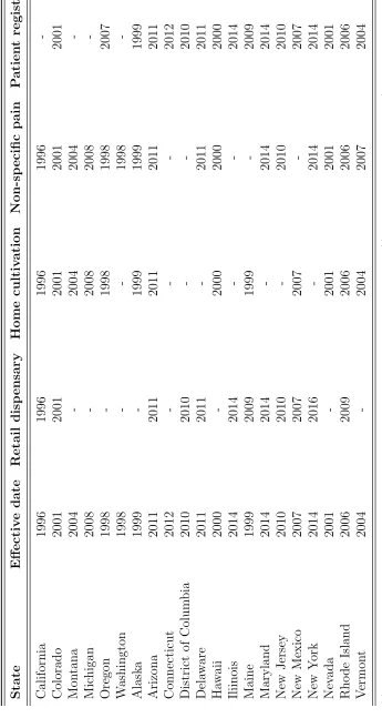
state-and year-level MML variables. As seen in Table 1.1, 23 states and D.C implemented

MMLs during the study period.

Since the literature suggests that there is relatively stronger evidence of marijuana

as a painkiller and the fact that the majority of medical marijuana patients use it for their

pain, specifically preferring it to opioid-based painkillers, I choose the main outcome variable

as the total amount of dollars spent on opioid-based medicines. Focusing on opioids is also

important from a policy perspective considering the costs associated with opioid misuse.

The key independent variables are indicators for MML implementation (effective

dates) in a given state and year and its individual components. As noted by Pacula et

al. (2015), MML states differ highly in how they allow medical marijuana and ignoring

the heterogeneities in these policy dimensions that exist both across time and states can

mask their heterogeneous effects and the mechanisms through which MMLs affect

utiliza-tion. Following Pacula et al. (2015) and Wen et al. (2015), I analyze the effects of four

key components that can lead to heterogeneity in prescription drug utilization: i) a “retail

dispensary” provision, an indicator of whether the state's MML explicitly allows/protects

dispensaries to dispense marijuana to medical marijuana patients, ii) a “home cultivation”

provision, an indicator of whether a state's MML allows the medical marijuana patient to

cultivate a certain amount of marijuana, iii) a “non-specific pain” provision, an indicator

of whether the state's MML lists any chronic pain or intractable pain in the eligible

condi-tions for medical marijuana instead of specifically listing the condicondi-tions associated with the

pain, and iv) a “patient registry” provision, an indicator for whether a state's MML requires

(29)

costs of obtaining medical marijuana of the patient as well as marijuana's perceived risk and

appropriateness for recommendation from the physician's view.

I control for individual and state level factors that are correlated with prescription

drug spending and with state decisions about MMLs. Individual-level covariates include a

rich set of sociodemographic and economic characteristics. State-level covariates include four

time-varying measures reflecting the variations in state economic conditions between 1996

and 2014: i) state unemployment rate, ii) state median household income, iii) state average

personal income, and iv) state uninsured rate. I include two policy variations during the

study period that can affect prescription drug spending and MML implementation. These

state-level policy variables include indicators for operational prescription drug monitoring

programs (PDMPs) and the implementation of a marijuana decriminalization/depenalization

in a state.

After pooling all the year, collapsing the prescribed opioid transactions at the

year-and person-level year-and excluding people under the age of 18, I have a sample of 435,035

person level observations. Tables 1.2 and 1.3 show the summary statistics for dependent and

independent variables.

1.4.1 Data characteristics and two-part model

Like other health care utilization data, prescription drug utilization distributions tend

to be skewed because 1) there cannot be negative spending, 2) there is a mass at point zero

for non-users, 3) patients with more severe conditions use substantially more on prescription

drugs than those with less severe conditions, and 4) there can be a small number of patients

with astronomical spending due to catastrophic health conditions. Health economists often

use log-transformed models to deal with these types of skewed outcomes. Other approaches

(30)

Certain transformations such as logging are not appropriate, especially when there is a large

mass of zeros. First, adding an arbitrary constant to observations is not recommended, and

second, using one-part models implicitly assume that observations with zero outcomes are

similarly affected by covariates as nonzero outcomes. These models are shown to behave

poorly compared to multi-part models (Duan et al. 1983; Mihaylova et al. 2011).

Due to the presence of the zero mass of non-users in the data, I use a two-part model

approach. The two-part model splits the prescription spending into two parts and applies

the basic rule of probability in estimating the parameters in the conditional mean function

E(y|x)=Pr(y>0|x)×E(y|y>0,x).

Figure 1.1 shows the nonlinearities in the distribution of opioid spending. There is a

large mass of non-users (approximately 90%), and the spending from users is skewed to the

right even after logging.

Since health care utilization data show heteroscedasticity, a re-transformation that

assumes homoscedastic, normally distributed log-scale error terms will give biased results.

Due to the complications that can arise with estimating the correct form of

heteroscedas-ticity, I avoid using OLS on logged outcomes with heteroscedastic retransformation and use

GLM for consistent estimation instead. The advantages of using GLM compared to models

with transformations are more broadly discussed in Manning and Mullahy (2001) and Jones

(2000).

GLM extends the classical linear models in two ways. First, it allows the dependent

variable to be distributed with any exponential family. Second, it allows for any monotonic

differentiable function of the dependent variable to vary linearly with the covariates (the link

function), rather than requiring the dependent variable itself to respond linearly (McCullagh

and Nelder 1989). Another advantage of using GLM is that it gives predictions on the raw

(31)

health care utilization and costs with GLM is a common approach in the literature (e.g.

Goda et al. 2011; Chandra et al. 2014; Strumpf et al. 2017).

For the baseline model, I use probit estimation, shown below, to estimate the

proba-bility of being a prescription drug user:

P r(Yiast>0|X) = Φ(Xβ)

where Yiast is the binary variable equal to one if the consumption for a person i living in

state s in year t for the drug category a is positive and zero otherwise. X is a vector of

explanatory variables including all the control variables in Table 3, state and year fixed

effects and state-specific linear time trends to capture the state-level factors that evolve over

time at a constant rate.

For the intensive margin, I use GLM models with log-link and gamma family to

estimate the amount of spending conditional on being a user as shown below:

E(Yiast|Yiast >0, X) = exp(Xγ)

where Yiast denotes the prescription drug spending for person i for drug categorya in state

s and year t, whileX denotes the same vector of covariates as in the first part.

As suggested by Manning and Mullahy (2001), I used modified Park tests to determine

the relationship between the conditional variance and the conditional mean functions, namely

the parameter δ in Var[Yiast|Yiast>0,X]=α[E(Yiast | Yiast >0, X)]δ. In all drug cases, ˆδ was

closest to 2 implying the gamma family.

Standard errors in all regressions are robust to heteroscedasticity and they are

(32)

the errors to be correlated within states while allowing them to be independent across states

(Bertrand et al. 2004).

As the main results, I report the combined marginal effects from both parts of the

model6

E(Yiast|X) = P r(Yiast|X >0)×E(Yiast |Yiast>0, X)

This setup models the difference in utilization on the original scale of the dependent

variable (dollar amount) yielding estimates that are readily interpretable. It also allows

for heteroscedasticity where Var(Expenditure|X) depends on the mean level of conditional

expenditures,E(Expenditure|X).

I also report the results from probability of use and amount of use separately. It

is possible that MMLs (and their provisions) have opposite effects on each margin of use,

especially if they act as an advertisement and encourage people to visit doctors who then

prescribe them drugs, increasing the probability of utilization, while decreasing the amount

of utilization by the users that are already on these drugs. If MMLs have opposite signs in

different parts, then it would be possible for the marginal effect to be significant in isolated

parts of the model along with the combined marginal effect being insignificant.

According to the CDC, prescription drug utilization is highest for people age 65 and

older, and there are substantial differences in utilization based on age. I stratified the sample

into three age groups because prescription drug utilization varies largely depending on age,

and lumping everyone in the same sample obscures this heterogeneity (Kantor et al. 2015).

The samples are ages 18-39 (N=186,144), 40-64 (N=180,723) and 65 and older (N=68,168).

Because there are stricter barriers for minors to obtain medical marijuana and the fact that

they are much less likely to have the conditions for which marijuana can be beneficial, I

exclude people younger than 18 from the sample.

6_{I used STATA}_'_{s twopm command developed by Belotti et al. 2015 to obtain the combined marginal}

(33)

1.5 Primary Results

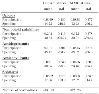
Table 2 presents the means of the main outcome variable of opioid spending along

with the drug categories that marijuana can potentially replace for the full sample. Both the

probability of any spending and the amount of spending conditional on positive spending on

opioids and other potentially marijuana substitutable prescriptions are lower in MML states

compared to control states.

To determine whether these differences are driven by MMLs, I estimate two different

models. First, I show results from the models that only include any MML, and in the second

I report the results from the model which only include its provisions. I also report a model

that simultaneously estimates all provisions and MML, but due to collinearity when the fixed

effects are included, I do not report these results as main findings.7

For my analyses I show results from two-part models instead of OLS on the whole

sample for three reasons. First, many people in these samples do not use these prescription

drugs, and part models explicitly model this large mass of non-users. Second, the

two-part model yields lower Akaike information criterion. Third, the two-two-part model gave better

out-of-sample predictions compared to OLS. I also run joint significance tests where the null

hypothesis is the coefficients from the four provisions of MMLs are jointly equal to zero

and report their p-values. I perform these tests for the models that include indicators for all

provisions and an indicator for existence of any MML. The motivation is to test whether these

provisions jointly explain variations which are not captured by a generic MML indicator.

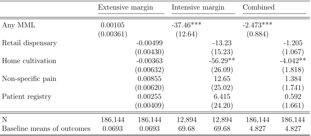
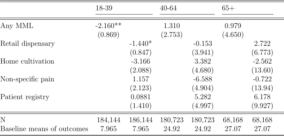
Tables 4 through 6 show the effects of a MML and its provisions on the different

margins of opioid spending among different age groups. According to the results in Table

4, a MML has no discernible effect on the probability of using opioids in young adults (ages

18-39). Although the coefficient on “any MML” is positive, it is insignificant. Similarly,

7_{Also, the interpretation of “any MML” becomes difficult in this model. These results are available upon}

(34)

none of the provisions show any discernible effects. However, there is a significant decrease

in opioid spending on the intensive margin. Namely, among young adult users of opioids

there is a decrease of $37.46 per person over a year associated with the passing of MML,

which translates to a 53.7% decrease from the baseline mean of opioid expenditures. Looking

at the model which includes its provisions we can see that “home cultivation” is the main

driver of this decrease with an even larger and significantly negative effect. Although “retail

dispensary” has negative effects, its coefficient is not precisely estimated. The last two

columns in Table 4 report the combined effects of MML and its provisions on the overall

population bringing the two parts together. Implementation of a MML significantly lowers

opioid spending in the overall population of young adults by $2.47 per person over a year.

Focusing on the effects of individual provisions in states where home cultivation is allowed,

young adults use $4 less of opioids per person holding all other provisions constant. The

“home cultivation” provision appears to be the main driver of the decreasing effect of MML

on opioids among young adults and these effects result from the intensive margin of use.

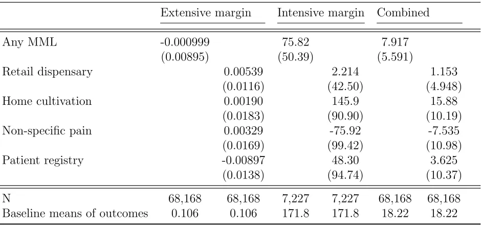
Tables 5 and 6 show there is not much evidence that a MML and its provisions significantly

change opioid spending among middle age (ages 40-64) and elderly people (ages 65+). The

only significant effect is found among middle age people. Namely, in states where the law

allows retail dispensaries, there is a 1.4% point drop in the probability of using opioids among

this group when we hold the other provisions fixed (a 14% decrease from the baseline mean).

As pointed out by earlier literature, most medical marijuana patients are younger adults so

it makes sense that we see a significant drop in opioid spending among younger populations

and almost no effect among older people.

The above analyses show independent effects of the four provisions, but states have

combinations of these provisions. Table 7 shows linear combinations of the marginal effects

from various combinations of the four provisions for each age group on the overall spending

(35)

effects of “home cultivation,” “non-specific pain” and “retail dispensary” provisions.

Cali-fornia is a state with this type of MML. CaliCali-fornia's type of MML is effective in reducing

opioid spending among young adults by $3.86 per person over a year and has no effect on

older populations. Second, I examine the effects of “retail dispensary,” “home cultivation,”

“non-specific pain” and “patient registry” provisions. Colorado is an example of a state with

such a MML. Colorado's type of MML is effective in reducing opioid spending among young

adults by $3.27 per person over a year. Next, I examine the combined effects of “retail

dispensary,” “non-specific pain” and “patient registry” provisions (New Jersey-type) and

combined effects of “home cultivation,” “non-specific pain” and “patient registry”

(Alaska-type). Both New Jersey's and Alaska's types of MML are not associated with any significant

decreases in reducing opioid spending.

A California-type MML which allows home cultivation, legalizes and protects

dispen-saries, and imposes no restrictions such as having a specific type of pain to be eligible or

requiring a registry of the patient is one of the least strict types of MML.8 It is also the

type of MML that reduces opioid spending the most among young adults, as measured by

the amount of dollar reduction in this study. Although not as loose as California's MML,

Colorado's type of MML is also one of the loosest models and associated with decreases in

opioid spending comparable to California's.

These results from the combined effects of provisions indicate the effects of MML

are not uniform but depend on the different combinations of provisions, consistent with

Pacula et al. (2015). The types of MMLs with the most generous provisions, which include

the protection and allowance of dispensaries with home cultivation, seem to be the most

effective types of MMLs in decreasing spending on opioid prescriptions.

8_{I also check whether the overall reductions in opioids were driven by California alone. The estimates}

(36)

1.6 Additional Analyses

Up to this point I have shown that the response of total prescription opioid

expendi-tures to MMLs depends on the age of the users and the margin of use. The point estimates

from combined marginal effects point decreases in spending on prescription opioids

associ-ated with MMLs among young adults. To further assess the validity of this finding, I perform

two types of sensitivity and two other additional analyses by exploring (i) the timing of the

policy implementation and policy endogeneity, (ii) the effects of MMLs on the number of

total opioid pills acquired instead of expenditures, (iii) the effects of MMLs and their

provi-sions on spending on other prescription drugs for which marijuana can potentially be used

as a substitute and (iv) the effects of MMLs and their provisions on prescription drugs for

which MMLs are not supposed to have any effect.

1.6.1 Event studies

Here I replicate my baseline specification with two-part models for expenditures on

opioids adding lead and lag indicators. This flexible event study approach enables me to

investigate whether there are any pre-existing trends in opioid expenditures which are

en-dogenous to MML adoption. Furthermore, it shows if the law has differential effects over

time after a MML is adopted. I exclude the indicator for the last year prior to MML adoption

and set it equal to zero for normalization.

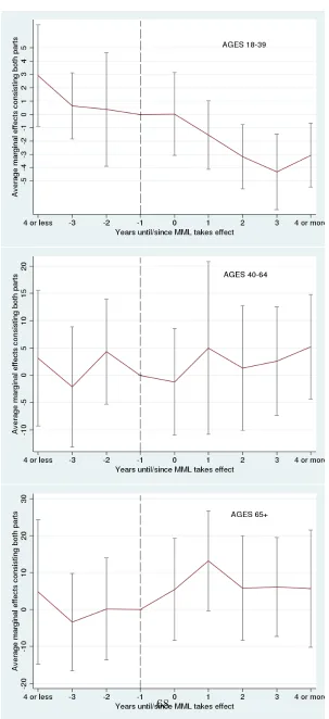
Figure 2 shows the estimated average marginal effects of the timing of the intervention

within four or more years before and after for each age group. The results for young adults

indicate there is a drop in prescription opioid expenditures after a year following the MML

adoption (relative to the year prior to adoption). The decreasing effect of a MML becomes

statistically significant after two years following the year it takes effect and continues to

(37)

maximum after three years. The decreasing impact of MML on opioids among young adults

is persistent over time with the long run difference being even larger than its instantenous

effect. There is not evidence of pre-existing trends: prior to intervention the effect of a MML

is indistinguishable from zero.

Turning to middle age and elderly populations there is not much evidence supporting

the hypothesis that a MML changes prescribed opioid expenditures over time. Among the

elderly population, a MML increases the opioid utilization after the first year of its adoption

(relative to the year prior to adoption), but this estimate is barely significant and it dissipates

the following years. There is not evidence of pre-trends before MML implementation in either

of these age groups.

These results from event study analyses support the main findings that MML

imple-mentation decreases the spending of prescription opioids among young adults but does not

have any discernible effect on older populations.

1.6.2 Effects on total number of opioid pills

So far, all the analyses were concerned with the expenditure outcomes for prescription

opioids. Although total expenditure is an important outcome from a government budget

spending perspective, it is not the only or the most complete measure of utilization. To

investigate whether the spending decreases in opioids associated with MMLs are attributed

to use rather than heterogeneous prescription drug prices, I perform analyses on total number

of prescribed opioid pills purchased using MEPS prescribed medicine files. Despite being an

imperfect measure of utilization, total number of prescribed opioid pills obtained can provide

some insights for the mechanisms of the effects found in main results.

Table 8 shows the average marginal effects of MMLs from two-part models on total

(38)

decreasing effect of “any MML” on opioid utilization remains. Namely, the mere adoption of

MML decreases the number of prescription opioid pills in the young population by 2.16 pills

per person over a year, which is a 27% decrease from the baseline mean. We can see that

decreases from “any MML” on opioids among young adults mainly result from the effects

from “home cultivation” and “retail dispensary” provisions. The effects of MML and its

provisions are null among the older populations when the outcome variable is number of

pills instead of total expenditures.

Comparing these results we see that the effects of MMLs found on opioid pills support

the primary results found on the opioid expenditures: implementation of MML decreases

opioid utilization among young adults.

1.6.3 Effects on the utilization of other prescription drugs

Although the majority of medical marijuana patients report using marijuana for pain,

there exists suggestive evidence on marijuana's effects on other health conditions.

Further-more, Reinerman et al. (2011) report the other common reasons patients cite for using

medical marijuana were muscle spasms, headache and anxiety. Reiman et al. (2017) report

mental health conditions were the second most common reason for using medical marijuana

after pain. In the light of these findings I study the effects of MMLs on other prescription

drugs for which marijuana can be a potential substitute.

The non-opioid prescription drugs I examine fall under four major groups: non-opioid

painkillers, antidepressants, anticonvulsants and sedatives. These categories of drugs are

commonly prescribed and they treat the conditions medical marijuana states render eligible.

They are also examined by earlier studies (Bradford and Bradford 2016 and 2017). If MMLs

are causing people to switch from their prescriptions to medical marijuana, utilization of

(39)

analyses only include Medicaid and Medicare recipients who incurred positive expenditures

of prescriptions. Here, l extend the analyses to a broader population.

Tables 9 through 11 show the combined marginal effects of “any MML” and MMLs'

four main provisions on expenditures for other marijuana-substitutable prescriptions for each

age group. The mere implementation of a MML has no impact on other drugs, except a

barely significant spending decrease in sedatives among young adults by $1.47 per person

over a year and a significant decrease in sedatives among the elderly by $6.75 per person

over a year.

Focusing on the effects of the four main provisions of MMLs, “retail dispensary” and

“home cultivation” provisions are generally associated with significant decreases on

antide-pressant and anticonvulsant expenditures among young adults and the elderly. Having a

“non-specific pain” provision in a state's MML is associated with a significant increase in

sedative spending among young adults. This increase in sedative spending results from the

increase in the extensive margin: having a “non-specific pain” provision increases the

proba-bility of sedative use significantly. This could be attributed to “non-specific pain” provision's

creation of ambiguities in eligibility criteria and extension of the patient base to people with

relatively milder pain (or no pain), who later end up being prescribed other prescriptions

upon seeing the physician. In fact, a “non-specific pain” provision also significantly increases

the probability of using antidepressants and anticonvulsants among young adults.9

Having a “patient registry” provision offsets the increasing effects of a “non-specific

pain” provision in young adults' sedative spending by decreasing it by $4.51 per person

over a year. It also decreases the elderly's sedative spending by $10.18 per person over a

year. The decreasing effect of a “patient registry” provision seems odd at first, but it could

be due to three reasons. First, requiring the registration of the patient could make the

recommendation of marijuana less risky from the physician's viewpoint, decreasing her cost

(40)

of recommending it. Similarly, being registered by the state and having a medical marijuana

patient identification card can decrease the patient's risk of arrest from carrying marijuana.

Looking at tables 9 and 11, it is natural to ask why sedatives are the drug category that is

most sensitive to these provisions in young adults and elderly. As pointed out in Proposition

5 MMLs' effects depend on the “mismatch” (or side effects) associated with a prescription

drug class and the health condition it treats. Sedatives along with opioids are reported to be

a class of drugs with the most severe side effects.10 Furthermore, mental health conditions

and anxiety are found to be the second most commonly reported reason for using medical

marijuana among medical marijuana patients (Reinerman et al. 2011 and Reiman et al.

2017). Therefore, a MML and its provisions can decrease sedative utilization more relative

to other categories of drugs with less severe side effects for which marijuana can substitute.

1.6.4 Placebo tests

Here, I check the effects of MMLs on drug classes for which marijuana has no potential

to substitute. I perform these analyses to demonstrate that negative effects of MML only

exist for the drug classes for which marijuana can be a substitute and not for the other drugs.

Tables 12 through 14 show results for some of the other commonly prescribed drugs on which

MMLs should not have any negative effect. The commonly prescribed placebo drugs include

hormones, hypertension drugs, cardiovascular agents and acid reducers. The results generally

support the hypothesis that MMLs and their provisions do not decrease expenditures on other

drugs, although there are some statistically significant increases, especially with middle age

and elderly people. “Patient registry” is linked with decreasing spending in one of the tests,

although it is only marginally significant at the 10% significance level.

10_{According to the CDC, sedatives were involved in 31.7% of drug-poisoning ER visits between 2008 and}

(41)

1.7 Conclusion

This paper shows that implementation of a MML by itself decreases opioid utilization

among young adults significantly, whether utilization is defined as spending or the number of

pills. Most of these reductions result from the intensive margin of utilization. The decreasing

effects of MMLs on opioids among young adults are persistent over time. They continue to

decrease opioid spending among young adults even four or more years after the year of their

implementation. The decreasing effects of MMLs are only observed among young adults

except for the allowance of retail dispensaries which decreases the probability of use among

middle age adults. MMLs also decrease sedative spending among the elderly. Given that

opioids and sedatives are the drug classes associated with the most severe cases of addiction

and adverse drug events, MMLs can be useful in alleviating the problematic use of these

prescriptions. Consistent with the prior literature, ignoring the heterogeneity in MMLs

can mask important effects of their individual provisions. States with the loosest MMLs

experience the biggest reductions in opioid utilization.

Despite growing trends of pro-marijuana policies, there remains a lack of scientific

evidence and consensus as to what extent marijuana affects health in the short and long

terms. Unlike prescription drugs, there are almost no guidelines on how to use marijuana

for medicinal purposes regarding its dosage, type, frequency and the method of its

consump-tion. Although states have been experimenting with different MMLs since 1996, conducting

randomized controlled experiments on marijuana with human subjects remains challenging

given its Schedule 1 categorization by the federal government.

There are several policy implications from this study. First, non-MML states with

high rates of opioid abuse and adverse drug events especially stemming from young adults

should look more carefully into adopting MMLs. Second, MML states should consider the

(42)

less likely to experience utilization reductions in prescribed opioids or other prescription

drugs, while less restrictive supply policies increase recreational use and abuse as found

by Pacula et al. (2015). This implies states should weigh the pros and cons of different

provisions when they design their MMLs according to their needs. Lastly, more research

is needed to inform policy makers on identifying the characteristics of medical marijuana

patients and why and how they use and substitute it. More randomized clinical trials are

also needed to assess the effects of marijuana on health so that physicians and patients are

(43)

Chapter 2 The Impact of Universal Coverage on

Health Care Utilization: Evidence

from Massachusetts

2.1 Introduction

The price elasticity of health care utilization is a great concern for economists and

pol-icymakers. Although there are a few randomized controlled trials investigating the impact

of cost sharing on health care utilization like the RAND and Oregon health insurance

ex-periments, these studies are outdated or limited to certain populations. Moreover, recent

reforms in health care markets raise questions about the impact of these insurance

expan-sions on utilization and health in the long term. The most recent insurance expansion is the

Affordable Care Act (ACA) which was enacted nationwide in 2014. However, years before

the ACA a very similar health insurance expansion reform took place in Massachusetts in

2006. The goal of the Massachusetts health care reform of 2006 was to achieve universal

health insurance by “incremental universalism”, which meant it would reduce the

uninsur-ance rate by filling the gaps in the existing system rather than ripping up the system and

Essays on Alternative Perspectives on Cross Border B2B Trust and Commitment

Georgia State University

ScholarWorks @ Georgia State University

Essays on Medical Marijuana Laws, Health

Insurance and Health Care Utilization

Pelin Ozluk

Table of Contents

List of Figures

List of Tables

Chapter 1

The Effects of Medical Marijuana

Laws on Utilization of Prescribed

Opioids and Other Prescription Drugs

1.1

Introduction

1.2

Background

1.2.1

Medical uses of marijuana and substitutability with opioids

1.2.2

Effects of MMLs and contribution of this study

1.3

Theoretical Framework

1.4

Estimation

1.4.1

Data characteristics and two-part model

1.5

Primary Results

1.6

Additional Analyses

1.6.1

Event studies

1.6.2

Effects on total number of opioid pills

1.6.3

Effects on the utilization of other prescription drugs

1.6.4

Placebo tests

1.7

Conclusion

Chapter 2

The Impact of Universal Coverage on

Health Care Utilization: Evidence

from Massachusetts

2.1

Introduction