R E S E A R C H
Open Access
A new method based on the
manifold-alternative approximating for
low-rank matrix completion
Fujiao Ren
1and Ruiping Wen
2**Correspondence:[email protected] 2Key Laboratory of Engineering &
Computing Science, Shanxi Provincial Department of Education/Department of Mathematics, Taiyuan Normal University, Shanxi, P.R. China Full list of author information is available at the end of the article
Abstract
In this paper, a new method is proposed for low-rank matrix completion which is based on the least squares approximating to the known elements in the manifold formed by the singular vectors of the partial singular value decomposition alternatively. The method can achieve a reduction of the rank of the manifold by gradually reducing the number of the singular value of the thresholding and get the optimal low-rank matrix. It is proven that the manifold-alternative approximating method is convergent under some conditions. Furthermore, compared with the augmented Lagrange multiplier and the orthogonal rank-one matrix pursuit algorithms by random experiments, it is more effective as regards the CPU time and the low-rank property.
Keywords: Manifold-alternative approximating; Low rank; Matrix completion; Convergence
1 Introduction
Matrix completion, proposed by Candès and Recht [7] in 2009, is a challenging problem. There has been a lot of study (see [1–8,11–19,23–28,30,33–35]) both in theoretical and algorithmic aspects on this problem. Explicitly seeking the lowest-rank matrix consistent with the known entries is mathematically expressed as
min
X∈Rn×nrank(X)
subject toXij=Mij, (i,j)∈Ω, (1.1)
where the matrixM∈Rn×nis the unknown matrix,Ωis a random subset of indices for
the known entries. The problem occurs in many areas of engineering and applied science, such as model reduction [20], machine learning [1,2], control [22], pattern recognition [10], imaging inpainting [3] and computer vision [29].
As is well known, Candés and Rechat [7] replaced the rank objective in (1.1) with its con-vex relaxation, and they showed that the lowest-rank matrices could be recovered exactly from most sufficiently large sets of sampled entries by computing the matrix of minimum nuclear norm that agreed with the provided entries, i.e., the exact matrix completion via
convex optimization, as follows:
min
X∈Rn×nX∗
subject toXij=Mij, (i,j)∈Ω, (1.2)
where the functionalX∗is the nuclear norm of the matrixX, the unknown matrixM∈
Rn×nofr-rank is square, and one has availablemsampled entries{M
ij: (i,j)∈Ω}withΩ
a random subset of cardinalitym.
There have been many algorithms which were designed to attempt to solve the global minimum of (1.2) directly. For example, the hard thresholding algorithms [4,15,17,26], the singular value theresholding (SVT) method [6], the accelerated singular values thresh-olding method (ASVT [14]), the proximal forward–backward splitting [9], the augmented Lagrange multiplier (ALM [19]) method, the interior point methods [7,28], and the new gradient projection (NGP [34]) method.
Based on the bi-linear decomposition of anr-rank matrix, some algorithms have been presented to solve (1.1) under ther-rank that is known or can be estimated [20,21]. We mention the Riemannian geometry method [30] and the Riemannian trust-region method [5, 23], the alternating minimization method [16] and the alternating steepest descent method [26]. The rank of many completion matrices, however, is unknown, so that one has to estimate it ahead of time or approximate it from a lower rank, which causes the difficulty of solving the matrix completion problem. Wen et al. [33] presented the two-stage iteration algorithms for the unknown-rank problem. To decrease the computational cost, based on extending the orthogonal matching pursuit (OMP) procedure from the vector to matrix level, Wang et al. [31] presented an orthogonal rank-one matrix pursuit (OR1MP) method, in which only the top singular vector pair was calculated at each iteration step and an -feasible solution can be obtained in onlyO(log(1)) iterations with less computational cost. However, the method converges to a feasible point rather than the optimal one with minimization rank such that the accuracy is poor and cannot be improved if the rank is reached. In this study, we come up with a manifold-alternative approximating method for solving the problem (1.2) motivated by the above. In an outer iteration, the approximated process can be done in the left-singular vector subspace and the approximation will be alternatively carried out in the right-singular vector subspace in an inner iteration. In a whole iteration, the reduction of the rank results in an alternating optimization, while the completed matrix satisfiesMij= (UVT)ij, for (i,j)∈Ω.
Here are some notations and preliminaries. LetΩ⊂ {1, 2, . . . ,n} × {1, 2, . . . ,n}denote the indices of the observed entries of the matrixX∈Rn×n,Ω¯ denote the indices of the missing entries.X∗ represents the nuclear norm (also called Schatten 1-norm) of X, that is, the sum of the singular values ofX,X2,XF denote 2-norm andF-norm ofX,
respectively. We denote byX,Y=trace(X∗,Y) the inner product between two matrices (X2
F=X,X). The Cauchy–Schwartz inequality givesX,Y ≤ XF·YFand it is well
known thatX,Y ≤ X2· Y∗[7,32]. For a matrixA∈Rn×n,vec(A) = (aT
1,aT2, . . . ,aTn)Tdenotes a vector reshaped from matrix Aby concatenating all its column vectors, dim(A) is always used to represent the dimen-sions ofAandr(A) stands for the rank ofA.
Sect.2. The convergence results of the new method are discussed in Sect.3. Finally, nu-merical experiments are shown with comparison to other methods in Sect.4. We end the paper with a concluding remark in Sect.5.
2 Methods
2.1 The method of augmented Lagrange multipliers
The method of augmented Lagrange multipliers (ALMs) was proposed in [19] for solving a convex optimization (1.2). It should be described subsequently.
Since the matrix completion problem is closely connected to the robust principal com-ponent analysis (RPCA) problem, it can be formulated in the same way as RPCA, an equiv-alent problem of (1.2) can be considered as follows.
As E will compensate for the unknown entries ofM, the unknown entries ofMare simply set as zeros. Suppose that the given data are arranged as the columns of a large matrixM∈Rm×n. The mathematical model for estimating the low-dimensional subspace
is to find a low-rank matrixX∈Rm×n, such that the discrepancy betweenX andMis
minimized, leading to the following constrained optimization:
min
X,E∈Rm×nX∗
subject toX+E=M, πΩ(E) = 0, (2.1)
whereπΩ:Rm×n→Rm×nis a linear operator that keeps the entries inΩunchanged and
sets those outsideΩ(say, inΩ) zeros. Then the partial augmented Lagrange function is
L(X,E,Y,μ) =X∗+Y,M–X–E+μ
2M–X–E 2
F.
The augmented Lagrange multipliers method is summarized in the following:
Method 2.1(Algorithm 6 of [19])
Input:Observation samplesMij, (i,j)∈Ω, of matrixM∈Rm×n.
1. Y0= 0;E0= 0;μ0> 0;ρ> 1;k= 0. 2. while not converged do
3. // Lines 4–5 solveAk+1=arg minXL(X,Ek,Yk,μk).
4. (U,S,V) =svd(M–Ek–μ–1k Yk);
5. Ak+1=USμ–1k [S]VT.
6. // Line 7 solvesEk+1=arg minπΩ(E)=0L(Ak+1,E,Yk,μk). 7. Ek+1=πΩ(M–Xk+1+μ–1k Yk).
8. Yk+1=Yk+μk(M–Xk+1–Ek+1). 9. Updateμktoμk+1.
10. k←k+ 1. 11. end while Output:(Xk,Ek).
Remark It is reported that the method of augmented Lagrange multipliers has been ap-plied to the problem (1.2). It is of much better numerical behavior, and it is also of much higher accuracy. However, the method has the disadvantage of the penalty function: the matrix sequences{Xk}generated by the method are not feasible. Hence, the accepted
2.2 The method of the orthogonal rank-one matrix pursuit (OR1MP)
We proceed based on the expression of the matrixX∈Rm×n,
X=M(θ) =
i∈Λ
θiMi, (2.2)
where{Mi:i∈Λ}is the set of allm×nrank-one matrices with unit Frobenius norm.
The original low-rank matrix approximation problem aims to minimize the zero-norm of the vectorθ= (θi)i∈Λsubject to the equality constraint
min
θ θ0
subject toPΩ
M(θ)=PΩ(Y), (2.3)
where θ0 represents the number of nonzero elements of the vector θ, andPΩ is the
orthogonal projector onto the span of matrices vanishing outside ofΩ. The authors in [31] reformulate further the problem as
minPΩ
M(θ)–PΩ(Y)
2
F
subject toθ0≤r, (2.4)
they could solve it by an orthogonal matching pursuit (OMP) type algorithm using rank-one matrices as the basis. It is implemented by two steps alternatively: rank-one is to pursue the basisMk, and the other is to learn the weight of the basisθk.
Method 2.2(Algorithm 1 of [31]) Input:YΩ and stopping criterion.
Initialize:SetX0= 0;θ0= 0 andk= 1.
repeat
Step 1: Find a pair of top left- and right-singular vectors(uk,vk)of the observed residual
matrixRk=YΩ–Xk–1and setMk=ukvTk.
Step 2: Compute the weight vectorθkusing the closed form least squares solutionθk=
(M¯T
kM¯k)–1M¯kTy˙. Step 3: SetXk=
k
i=1θik(Mi)Ω andk←k+ 1.
untilstopping criterion is satisfied
Output:Constructed matrixYˆ=ki=1θikMi.
Remark To decrease the computational cost, based on extending the orthogonal match-ing pursuit (OMP) procedure from the vector to matrix level, Wang et al. [31] presented an orthogonal rank-one matrix pursuit (OR1MP) method, in which only the top singular vector pair was calculated at each iteration step and an-feasible solution can be obtained in onlyO(log(1
)) iterations with less computational cost. However, the method converges
2.3 The method of a manifold-alternative approximating (MAA)
For convenience, [Uk,Σk,Vk]τk=lansvd(Yk) denotes the top-τksingular pairs of the matrix
Ykby using the Lanczos method, whereUk= (u1,u2, . . . ,uτk),Vk= (v1,v2, . . . ,vτk) andΣk= diag(σ1k,σ2k, . . . ,στk,k),σ1k≥σ2k≥ · · · ≥στk,k> 0.
Let
Mk=
X∈Rn×m:rank(X) =k
denote the manifold of fixed-rank matrices. Using the SVD, one has the equivalent char-acterization
Mk=
UΣVT:U∈Stkm,V∈Stnk,Σ=diag(σi),σ1≥ · · · ≥σk> 0
, (2.5)
whereStm
k is the Stiefel manifold ofm×kreal, orthogonal matrices, anddiag(σi) denotes
a diagonal matrix withσi,i= 1, 2, . . . ,kon the diagonal.
Method 2.3(MAA)
Input:D=PΩ(M),vec(D) =D(i,j), (i,j)∈Ω,τ0> 0 (τk∈N+), 0 <c1,c2< 1, a tolerance > 0.
Initialize:SetY0=Dandk= 0.
repeat
Step 1: Compute the partial SVD of the matrixYk: [Uk,Σk,Vk]τk=lansvd(Yk).
Step 2: Solve the following optimization models,minvec(D) –vec(PΩ(UkXk))F, set Yk+1=UkXk.
Step 3: WhenYk+1–YkF
DF <, stop; otherwise, go to the next step.
Step 4: Fork> 0, ifvec(D) –vec(PΩ(Yk+1))F<c2vec(D) –vec(PΩ(Yk))F,τk+1= [c1τk]
go to the next step; otherwise, do
(1): SetZk=D+PΩ(Yk+1), compute the partial SVD of the matrixZk:
[Uk,Σk,Vk]τk=lansvd(Zk). Let
WK=UkΣkVkT,αk=vec(D) –vec(PΩ(Wk))F.
SetZk+1
2 =D+PΩ(Wk).
(2): Do SVD:
[Uk+1
2,Σk+12,Vk+21]τk=lansvd(Zk+12).
ThenWk+1
2 =Uk+12Σk+12V
T k+12.
(3): Solve the following minimum problems, yieldingYk+1
2 andαk+12,
minvec(D) –vec(PΩ(Xk+1 2V
T
k+12))F, setYk+12 =Xk+12V
T k+12, αk+1
2 =vec(D) –vec(PΩ(Yk+12))F.
SetZk+1=D+PΩ(Yk+12). (4): Ifαk+1
2 ≤c2αk,τk+1=τk– 1; ifαk+12 ≥αk,τk+1=τk+ 1, go to Step 1.
Otherwise, ifc2αk≤αk+12 <αk,τk+1=τk, go to the next step. Step 5: k:=k+ 1, go to Step 2.
untilstopping criterion is satisfied
3 Convergence analysis
Now, the convergence theory will be discussed in the following.
Lemma 3.1 Let Y∗be the optimal solution of(1.1).Then there exists a nonnegative number
ε0such that
Y–Y∗
F≥ε0
if and only if for any matrix Y,r(Y) <r(Y∗).
Proof From the discretional nature of the rank, there existsYεthat satisfies
r(Yε)≤r(Y) – 1, ∀ε> 0,
and
Yε–Y∗F<ε.
Hence,Yε→Y∗ifε→0.
This is in contrast tor(Y∗)≤r(Y∗) – 1.
Lemma 3.2 Assume that the manifolds Wk+1
2,Wksatisfy
r(Wk+1
2)≥r(Wk),
then
αk+1 2 <αk.
Furthermore,αk+1
2 ≤cαkif there exists a number c(0 <c< 1)that satisfies
PΩ¯(Yk+21 –Wk+12)F≥(1 –c)Yk+12–Wk+12F.
Proof From Method2.3, we can see that
αk+1
2 ≤vec(D) –vec
PΩ(Wk+1
2)F=vec
PΩ(Yk+1
2)
–vecPΩ(Wk+1 2)F
=Yk+1
2 –Wk+12F–PΩ¯(Yk+12 –Wk+12)F.
When
PΩ¯(Yk+21 –Wk+12)F≥(1 –c)Yk+12–Wk+12F,
we have
αk+1
2 ≤cYk+12 –Wk+12F≤cYk+12 –WkF
=cPΩ(Yk) –PΩ(Wk)F=cvec(D) –vec
Ifc= 1,
PΩ¯(Y
k+12 –Wk+12)F≥0
holds true. Thus,
αk+1 2 <αk
is true.
Lemma 3.3 Assume that{Yk}is the feasible matrix sequence generated by Method2.3, {Wk}is the low-dimensional matrix sequence formed by partial singular pairs,then
lim
k→∞Yk–WkF= 0
if the following conditions are satisfied:
r(Wk) =r and PΩ¯(Yk–Wk)F≥(1 –c)Yk–WkF.
Proof From
Yk–WkF≤ Yk–Wk–1F
=PΩ(Yk–Wk–1)F
≤cYk–1–Wk–1F ≤ · · ·
≤ckY0–W0F.
Therefore,
lim
k→∞Yk–WkF= 0
holds true.
Theorem 3.1 Assume that there exists a positive number c(0 <c< 1)such that the feasible matrices Yksatisfy the following inequality:
PΩ¯(Yk–Wk)F≥(1 –c)Yk–WkF, (3.1)
then the iteration matrices sequence{Yk}generated by Method2.3converges to the optimal solution Y∗of(1.2)when the terminated rule→0is satisfied.
Proof From the Method2.3, we can see the following:
Case I.τk+1= [c1τk] if
vec(D) –vecPΩ(Yk+1)F≤c2vec(D) –vec
holds true. That is,
dim(Wk+1) <dim(Wk),
whereWk+1=Uk+1Σk+1VkT+1.
Therefore, there exists an indexk0such thatr(Wk0) <r(Y∗).
From Lemma3.1, the inequality (3.1) holds true.
At that time, the procedure can be transferred into Step 4 of Method2.3, and thenτk0+1=
τk0+ 1; repeat it, there exists an indexk1such thatr(Wk1) =r(Y∗).
Because of the assumption (3.1) and Lemma3.2,
lim
αk→0D–PΩ(Yk)F= 0
is true under the restricted conditionr(Wk) =r(Y∗),k>k1. From Lemma3.3, we have
lim
k→∞Wk–YkF= 0.
Hence,
lim
k→∞Yk=klim→∞Wk=Y
∗.
Case II. We assume that there exists an indexk2such that the inequality (3.1) holds false butr(Wk2) >r(Y∗), and then the procedure can be transferred into the Step 4 of Method 2.3. Because of the assumption (3.1) and Lemma3.2, we know that there exists an index
k3such that the following holds true:
αk
3+12 <min{α1,α2, . . . ,αk3}.
At that time,τk3+1=τk3– 1, say, the number of dimensionality is decreasing. Repeat the
above again and again until there exists an indexk4such thatr(Wk4) =r(Y∗).
That is, we always have the following:
lim
k→∞Yk=klim→∞Wk=Y
∗.
The theorem has been proved.
4 Numerical experiments
It is well known that the OR1MP methd is the most simple and efficient for solving prob-lem (1.1) and the ALM method is one of the most popular and efficient methods for solving problem (1.2). In this section we test several experiments to analyze the performance of our Method2.3, and compare with the ALM and OR1MP methods.
We compare the methods using general matrix completion problem. In the experiments,
p=m/n2denotes the observation ratio, wheremis the number of observed entries. Here,
p= 0.1, 0.2, 0.3, 0.5 are the different choices of the above ratio. The relative error is RES = Yk–DF
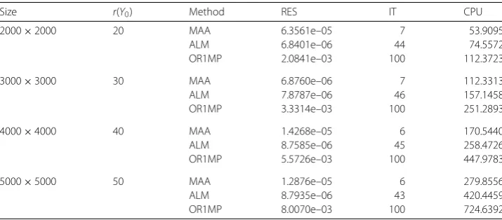
The results of the experiments are presented in Tables1–4. From Tables1–4we can see that Method2.3takes much fewer iterations (denoted by “IT”)) and requires much less computational time (denoted by CPU) than the ALM and OR1MP methods. Thus, Method2.3is much more efficient than the other two methods.
Table 1 Comparison results of three methods forp= 0.1
Size r(Y0) Method RES IT CPU
2000×2000 20 MAA 6.3989e–05 19 61.0538
ALM 1.3289e–05 147 814.4656
OR1MP 1.5920e–02 100 80.2022
3000×3000 30 MAA 2.4436e–04 15 113.8439
ALM 1.2810e–05 155 3448.8579
OR1MP 1.5641e–02 100 177.3123
4000×4000 40 MAA 1.2204e–04 13 163.4071
ALM 1.1951e–05 166 9876.8939
OR1MP 1.8042e–02 100 318.5400
5000×5000 50 MAA 5.3731e–05 11 210.7015
ALM 9.6254e–06 173 22,641.7724
[image:9.595.118.478.378.534.2]OR1MP 2.0254e–02 100 505.3112
Table 2 Comparison results of three methods forp= 0.2
Size r(Y0) Method RES IT CPU
2000×2000 20 MAA 2.4308e–04 10 54.8639
ALM 9.2238e–06 70 237.4327
OR1MP 4.3432e–03 100 95.9820
3000×3000 30 MAA 5.0593e–05 8 94.3904
ALM 5.6067e–05 72 863.4068
OR1MP 5.9270e–02 100 213.9196
4000×4000 40 MAA 1.3172e–04 8 166.8769
ALM 5.4632e–06 72 2336.2629
OR1MP 8.5351e–03 100 382.8628
5000×5000 50 MAA 9.1096e–06 8 248.6944
ALM 1.0802e–05 64 5141.8507
OR1MP 1.1188e–02 100 603.1532
Table 3 Comparison results of three methods forp= 0.3
Size r(Y0) Method RES IT CPU
2000×2000 20 MAA 6.3561e–05 7 53.9095
ALM 6.8401e–06 44 74.5572
OR1MP 2.0841e–03 100 112.3723
3000×3000 30 MAA 6.8760e–06 7 112.3313
ALM 7.8787e–06 46 157.1458
OR1MP 3.3314e–03 100 251.2893
4000×4000 40 MAA 1.4268e–05 6 170.5440
ALM 8.7585e–06 45 258.4726
OR1MP 5.5726e–03 100 447.9783
5000×5000 50 MAA 1.2876e–05 6 279.8556
ALM 8.7935e–06 43 420.4459
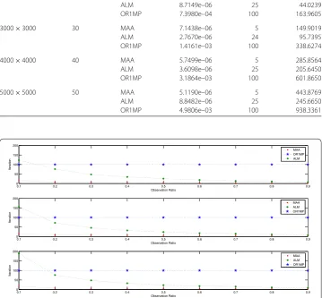
[image:9.595.118.476.575.732.2]Table 4 Comparison results of three methods forp= 0.5
Size r(Y0) Method RES IT CPU
2000×2000 20 MAA 1.2636e–05 5 65.7244
ALM 8.7149e–06 25 44.0239
OR1MP 7.3980e–04 100 163.9605
3000×3000 30 MAA 7.1438e–06 5 149.9019
ALM 2.7670e–06 24 95.7395
OR1MP 1.4161e–03 100 338.6274
4000×4000 40 MAA 5.7499e–06 5 285.8564
ALM 3.6098e–06 25 205.6450
OR1MP 3.1864e–03 100 601.8650
5000×5000 50 MAA 5.1190e–06 5 443.8769
ALM 8.8482e–06 25 245.6650
OR1MP 4.9806e–03 100 938.3361
Figure 1Comparison of completion performance of the MAA, ALM, OR1MP methods with different percentages of observations: the figures correspond to the results on three 3000×3000 random matrices of rank 10 (top figure), rank 30 (middle figure), rank 50 (bottom figure)
In order to display the effectiveness of our method further, we conduct an experiment on a 3000×3000 matrix with three different ranks 10, 30, 50 for three methods with the observation ratios ranging from 0.1 to 0.9, as shown in Fig.1.
5 Concluding remark
Based on the least squares approximation to the known elements, we proposed a manifold-alternative approximating method for the low matrix completion problem. Compared with the ALM and OR1MP methods, shown in Tables1–4, our method performs bet-ter as regards the computing time and the low-rank property. The method can achieve a reduction of the rank of the manifold by gradually reducing the number of the singular value of the thresholding and get the optimal low-rank matrix each iteration step.
Acknowledgements
[image:10.595.118.478.122.455.2]Funding
It is not applicable.
Abbreviations
OMP, orthogonal matching pursuit; OR1MP, orthogonal rank-one matrix pursuit; SVD, singular value decomposition; SVT, singular value theresholding; ASVT, accelerated singular values thresholding method; ALM, augmented Lagrange multiplier; NGP, new gradient projection; RPCA, robust principal component analysis; MAA, manifold-alternative approximating; IT, iteration number; RES, relative errors; CPU, computing time.
Availability of data and materials
Please contact author for data requests.
Competing interests
The authors declare that they have no competing interests.
Authors’ contributions
All authors contributed equally to the writing of this paper. All authors read and approved the final manuscript.
Author details
1Department of Mathematics, Taiyuan Normal University, Shanxi, P.R. China.2Key Laboratory of Engineering & Computing
Science, Shanxi Provincial Department of Education/Department of Mathematics, Taiyuan Normal University, Shanxi, P.R. China.
Publisher’s Note
Springer Nature remains neutral with regard to jurisdictional claims in published maps and institutional affiliations.
Received: 18 September 2018 Accepted: 3 December 2018 References
1. Amit, Y., Fink, M., Srebro, N., Ullman, S.: Uncovering shared structures in multiclass classification. In: Proceeding of the 24th International Conference on Machine Learning, pp. 17–24. ACM, New York (2007)
2. Argyriou, A., Evgeniou, T., Pontil, M.: Multi-task feature learning. Adv. Neural Inf. Process. Syst.19, 41–48 (2007) 3. Bertalmio, M., Sapiro, G., Caselles, V., Ballester, C.: Multi-task feature learning, image inpainting. Comput. Graph.34,
417–424 (2000)
4. Blanchard, J., Tanner, J., Wei, K.: CGIHT: conjugate gradient iterative and thresholding for compressed sensing and matrix completion. In: Numerical Analysis Group (2014) Preprint 14/08
5. Boumal, N., Absil, P.A.: RTRMC: a Riemannian trust-region method for low-rank matrix completion. In: Shawe-Taylor, J., Zemel, R.S., Bartlett, P., Pereira, F.C.N., Weinberger, K.Q. (eds.) Advances in Neural Inf. Processing Systems, NIPS, vol. 24, pp. 406–414 (2011)
6. Cai, J.-F., Candès, E.J., Shen, Z.: A singular value thresholding method for matrix completion. SIAM J. Optim.20(4), 1956–1982 (2010)
7. Candès, E.J., Recht, B.: Exact matrix completion via convex optimization. Found. Comput. Math.9(6), 717–772 (2009) 8. Candès, E.J., Tao, T.: The power of convex relaxation: near-optimal matrix completion. IEEE Trans. Inf. Theory56(5),
2053–2080 (2009)
9. Combettes, P.L., Wajs, V.R.: Signal recovered by proximal forward–backward splitting. Multiscale Model. Simul.4, 1168–1200 (2005)
10. Eldén, L.: Matrix Methods in Data Mining and Pattern Recognization. Society for Industrial and Applied Mathematics, Philadelphia (2007)
11. Fazel, M.: Matrix rank minimization with applications. Ph.D. Dissertation, Stanford University (2002)
12. Haldar, J.P., Hernando, D.: Rank-constrained solutions to linear matrix equations using PowerFactorization. IEEE Signal Process. Lett.16(7), 584–587 (2009)
13. Harvey, N.J., Karger, D.R., Yekhanin, S.: The complexity of matrix completion. In: Proceeding of the Seventeenth Annual ACM-SIAM Symposium on Discrete Algorithms, SODA, pp. 1103–1111 (2006)
14. Hu, Y., Zhang, D.-B., Liu, J., Ye, J.-P., He, X.-F.: Accelerated singular value thresholding for matrix completion. In: KDD’12, Beijing, China, August 12–16, 2012 (2012)
15. Jain, P., Meka, R., Dhillon, I.: Guaranteed rank minimization via singular value projection. In: Proceeding of the Neural Information Processing Systems Conf., NIPS, pp. 937–945 (2010)
16. Jain, P., Netrapalli, P., Sanghavi, S.: Low-rank matrix completion using alternating minimization. In: Proceedings of the 45th Annual ACM Symposium on Theory of Computing (STOC), pp. 665–674 (2013)
17. Kyríllidis, A., Cevher, V.: Matrix recipes for hard thresholding methods. J. Math. Imaging Vis.48(2), 235–265 (2014) 18. Lai, M.-J., Xu, Y., Yin, W.: Improved iteratively reweighted least squares for unconstrained smoothedlqminimization.
SIAM J. Numer. Anal.51, 927–957 (2013)
19. Lin, Z.-C., Chen, M.-M., Ma, Y.: A fast augmented Lagrange multiplier method for exact recovery of corrupted low-rank matrices. In: Proceeding of the 27th International Conference on Machine Learning, Haifa, Israel (2010)
20. Liu, Z., Vandenberghe, L.: Interior-point method for nuclear norm approximation with application to system identification. SIAM J. Matrix Anal. Appl.31, 1235–1256 (2009)
21. Lu, Z., Zhang, Y.: Penalty decomposition methods for rank minimization (2010)https://arxiv.org/abs/1008.5373
22. Mesbahi, M., Papavassilopoulos, G.P.: On the rank minimization problem over a positive semidefinite linear matrix inequality. IEEE Trans. Autom. Control42, 239–243 (1997)
23. Mishra, B., Apuroop, K.A., Sepulchre, R.: A Riemannian geometry for low-rank matrix completion (2013)
24. Ngo, T., Saad, Y.: Scaled gradients on Grassmann manifolds for matrix completion. In: Advances in Neural Information Processing Systems, NIPS, (2012)
25. Recht, B., Fazel, M., Parrilo, P.A.: Guaranteed minimum-rank solutions of linear matrix equations via nuclear norm minimization. SIAM Rev.52(3), 47–501 (2010)
26. Tanner, J., Wei, K.: Low-rank matrix completion by alternating steepest descent methods. Appl. Comput. Harmon. Anal.40, 417–429 (2016)
27. Toh, K.C., Todd, M.J., Tutuncu, R.H.: SDPTS-a Matlab software package for semidefinite-quadratic-linear programming (2001) version 3.0, Web pagehttp://www.math.nus.edu.sg/mattohkc/sdpt3.html
28. Toh, K.C., Yun, S.: An accelerated proximal gradient algorithm for nuclear norm regularized linear least squares problems. Pac. J. Optim.6, 615–640 (2010)
29. Tomasi, C., Kanade, T.: Shape and motion from image streams under orthography: a factorization method. Int. J. Comput. Vis.9, 137–154 (1992)
30. Vanderreycken, B.: Low rank matrix completion by Riemannian optimization. SIAM J. Control Optim.23(2), 1214–1236 (2013)
31. Wang, Z., Lai, M.-J., Lu, Z.-S., Fan, W., Hansan, D., Ye, J.-P.: Orthogonal rank-one matrix pursuit for low rank matrix completion. SIAM J. Sci. Comput.37, 488–514 (2015)
32. Waston, G.A.: Characterization of subdifferential of some matrix norms. Linear Algebra Appl.170, 33–45 (1992) 33. Wen, R.-P., Liu, L.-X.: The two-stage iteration algorithms based on the shortest distance for low rank matrix
completion. Appl. Math. Comput.314, 133–141 (2017)
34. Wen, R.-P., Yan, X.-H.: A new gradient projection method for matrix completion. Appl. Math. Comput.258, 537–544 (2015)
35. Wen, Z., Yin, W., Zhang, Y.: Solving a low-rank factorization model for matrix completion by a non-linear successive over-relaxation algorithm. Math. Program. Comput.4, 333–361 (2012)