R E S E A R C H
Open Access
Weak convergence of explicit extragradient
algorithms for solving equilibirum problems
Habib ur Rehman
1, Poom Kumam
1,2*, Yeol Je Cho
3and Pasakorn Yordsorn
1*Correspondence:
1Department of Mathematics, King
Mongkut’s University of Technology Thonburi (KMUTT), Bangkok, Thailand
2Center of Excellence in Theoretical
and Computational Science (TaCS-CoE), SCL 802 Fixed Point Laboratory, King Mongkut’s University of Technology Thonburi (KMUTT), Bangkok, Thailand Full list of author information is available at the end of the article
Abstract
This paper aims to propose two new algorithms that are developed by implementing inertial and subgradient techniques to solve the problem of pseudomonotone equilibrium problems. The weak convergence of these algorithms is well established based on standard assumptions of a cost bi-function. The advantage of these algorithms was that they did not need a line search procedure or any information on Lipschitz-type bifunction constants for step-size evaluation. A practical explanation for this is that they use a sequence of step-sizes that are updated at each iteration based on some previous iterations. For numerical examples, we discuss two
well-known equilibrium models that assist our well-established convergence results, and we see that the suggested algorithm has a competitive advantage over time of execution and the number of iterations.
MSC: 65Y05; 65K15; 47H05; 47H10
Keywords: Equilibrium problem; Extragradient method; Lipschitz-type conditions; Nash–Cournot equilibrium model of electricity markets
1 Introduction
Equilibrium problem (shortly,EP) can be considered as a general problem in the sense that it comprises many mathematical models such as variational inequality problems (shortly, VIP), optimization problems, fixed point problems, complementarity problems, Nash equilibrium of noncooperative games, saddle point, vector minimization problem and the Kirszbraun problem (see e.g., [1–4]). To the best of our knowledge, the term “equilibrium problem” was initiated in 1992 by Mu and Oettli [5] and has been further strengthened by Blum and Oettli [1]. The equilibrium problem (EP) is also seen as the Ky Fan inequality, since Fan [6] gives the first existence result regarding the solution of theEP. Many results about the existence of the solution of equilibrium problems have been accomplished and generalized by several authors (e.g., see [7,8]). One of the most useful research directions in the equilibrium problem theory is to develop the iterative methods to find a numeri-cal solution of the equilibrium problems. The research in this direction is continuing to develop new methods, leading weak convergence to strong convergence, providing mod-ification and extension of existing algorithms which are suitable for a specific subclass of equilibrium problems. In recent years, many methods have been developed to solve equi-librium problems in finite and infinite-dimensional spaces (for instance, [9–20]).
In this direction, two approaches are very well known, one of them is the proximal point method (shortly,PPM) [21] and the other one is an auxiliary problem principle [22]. The PPMwas introduced by Martinet [23] for monotone variational inequality problems, and later it was continued by Rockafellar [24] for monotone operators. Moudafi [21] extended the PPM toEPs involving monotone bifunction. ThePPM method is implemented to monotoneEPs, i.e. the bifunction of an equilibrium problem has to be monotone. Thus, each regularized subproblem becomes strongly monotone, and a unique solution exists. This method will not guarantee the existence of the solution if the bifunction is more gen-eral monotone, like pseudomonotone. However, the auxiliary problem principle is based on the idea to develop a new problem that is identical and usually simpler to solve com-pared to the initial problem. This principle was early established by Cohen [25] for opti-mization problems and later extended for variational inequality problems [26]. Moreover, Mastroeni [22] uses the auxiliary problem principle for strongly monotone equilibrium problems.
In this paper, we focus on the second direction, including projection methods that are well known and practically easy to implement due to their easier numerical computation. As is well known, the earliest well-known projection method forVIPs is the gradient pro-jection method. After that, many other propro-jection methods were developed such as the extragradient method [27], the subgradient extragradient method [28], Popov’s extragra-dient method [29], Tseng’s extragradient method [30], projection and contraction schemes [31] and other hybrid and projected gradient methods [32–35]. In recent years, the equi-librium problem theory has become an attractive field for many researchers and a lot of numerical methods for solving equilibrium problems have been developed and analyzed by many authors in Hilbert spaces. Thus, Quoc [20] and Flam [36] extended the extragra-dient method for equilibrium problems. Recently, Hieu [37] extended the Halpern subgra-dient extragrasubgra-dient method for variational inequality problem to an equilibrium problem and also many other methods were extended and modified for variational inequality prob-lems to equilibrium probprob-lems (see [38,39]).
On the other hand, let us point out inertial-type algorithms, depending on the heavy ball methods of the two-order time dynamical system, Polyak [40] firstly proposed an in-ertial extrapolation as an acceleration process to solve the smooth convex minimization problem. The inertial method is a two-step iterative method, and the next iteration is de-termined by the use of two previous iterates and it can be considered as a procedure of speeding up an iterative sequence (for more details, see [40,41]). Various inertilike al-gorithms previously developed for special classes of the problem (EP) can be found (for instance, in [42–44]). For the problem (EP), Moudafi [45] has done work in this direction and proposed a new inertial-type method, namely the second-order differential proximal method. This algorithm can be taken as a combination of the relaxedPPM[21] and in-ertial effect [40]. Recently, another type of inertial algorithm has also been introduced by Chbani and Riahi [46], by choosing a suitable inertial term and incorporating a viscosity-like technique in their algorithm.
of line search procedures and also there is no need to have a prior knowledge of Lipschitz-type constants of a bifunction. Instead of that, they use a sequence of step-sizes which is updated at each iteration, based on some previous iterates. We establish the weak conver-gence of the resulting algorithm under standard assumptions on a cost bifunction.
We organize the rest of this paper in the following manner: In Sect.2, we give some definitions and preliminary results that will be used throughout the paper. Section3 com-prises our first subgradient algorithm and provides the weak convergence theorem for the proposed algorithm. Section4deals with proposing and analyzing the convergence of the inertial subgradient algorithm, involving a pseudomonotone bifunction. Finally, in Sect. 5, we study the numerical experiments to illustrate the computational perfor-mance of our suggested algorithms on test problems, which are modeled from a Nash– Cournot oligopolistic equilibrium model and Nash–Cournot equilibrium models of elec-tricity markets.
2 Preliminaries
LetCbe a closed and convex subset of a Hilbert spaceHwith an inner product·,·and norm · , respectively. LetRbe the set of all real numbers andNbe the set all positive integers. While{xn}is a sequence inH, we denote the strong convergence byxn→xand
weak convergence by xnxasn→ ∞. Also, [t]+=max{0,t} andEP(f,C) denote the
solution set of the equilibrium problem insideCandpis an element ofEP(f,C).
Definition 2.1(Equilibrium problem [1]) LetCbe a nonempty closed convex subset of
H. Letf be a bifunction fromC×Cto the set of real numbersRsuch thatf(x,x) = 0 for allx∈C. The equilibrium problem (EP) for the bifunctionf onCis to
Findp∈C such that f(p,y)≥0, ∀y∈C.
Definition 2.2 ([50]) LetCbe a closed convex subset in H and we denote the metric projection onCbyPC(x),∀x∈H, i.e.
PC(x) =arg min
y–x:y∈C.
Lemma 2.1([51]) Let PC:H→C be the metric projection fromHonto C.Then (i) For allx∈C,y∈H,
x–PC(y)2+PC(y) –y2≤ x–y2.
(ii) z=PC(x)if and only if
x–z,y–z ≤0.
Now, we define concepts of monotonicity for a bifunction (see [1,52] for more details).
Definition 2.3 A bifunctionf:H×H→Ris said to be
(i) strongly monotoneonCif there exists a constantγ> 0such that
(ii) monotoneonCif
f(x,y) +f(y,x)≤0, ∀x,y∈C;
(iii) strongly pseudomonotoneonCif there exists a constantγ > 0such that
f(x,y)≥0 ⇒ f(y,x)≤–γx–y2, ∀x,y∈C;
(iv) pseudomonotoneonCif
f(x,y)≥0 ⇒ f(y,x)≤0, ∀x,y∈C;
(v) a Lipschitz-type conditiononCif there exist two positive constantsc1,c2such that
f(x,z)≤f(x,y) +f(y,z) +c1x–y2+c2y–z2, ∀x,y,z∈C.
Remark2.1 From Definition2.3, the following implications hold:
(i)⇒(ii)⇒(iv) and (i)⇒(iii)⇒(iv).
Remark2.2 The converse of the above implications is not true in general.
Remark2.3 IfF:C→His a Lipschitz continuous operator, then the bifunctionf(x,y) = F(x),y–xsatisfies Lipschitz-type condition withc1=c2=L2 (see [53], Lemma 6(i)).
Further, we recall that thesubdifferentialof a convex functiong:C→Ratx∈Cis defined by
∂g(x) =w∈C:g(y) –g(x)≥ w,y–x,∀y∈C,
and thenormal coneofCatx∈Cis defined by
NC(x) =
w∈H:w,y–x ≤0,∀y∈C.
Lemma 2.2([54], p. 97) Let C be a nonempty closed convex subset of a real Hilbert space
Hand g:C→Rbe a convex,subdifferentiable,lower semicontinuous function on C.Then z is a solution to the following convex optimization problemmin{g(x) :x∈C}if and only if 0∈∂g(z) +NC(z),where∂g(z)and NC(z)denote the subdifferential of g at z and the normal
cone of C at z,respectively.
Lemma 2.3([55], p. 31) For all x,y∈Hwithμ∈Rthe following relation holds:
μx+ (1 –μ)y2=μx2+ (1 –μ)y2–μ(1 –μ)x–y2.
Lemma 2.4([56]) Letφn,δnandβnbe sequences in[0, +∞)such that
φn+1≤φn+βn(φn–φn–1) +δn, ∀n≥1,
+∞
n=1
and there exists a real number β with0≤βn≤β< 1for all n∈N.Then the following
relations hold:
(i) +n=1∞[φn–φn–1]+<∞,where[t]+:=max{t, 0}.
(ii) There existsφ∗∈[0, +∞)such thatlimn→+∞φn=φ∗.
Lemma 2.5([57]) Let C be a nonempty set ofHand{xn}be a sequence inHsuch that the
following two conditions hold:
(i) For everyx∈C,limn→∞xn–xexists.
(ii) Every sequentially weak cluster point of{xn}is inC.
Then{xn}converges weakly to a point in C.
Assumption 2.1 We have the following assumptions on the bifunctionf :H×H→R which are useful to prove the weak convergence of the iterative sequence{xn}generated
by our proposed algorithms.
(A1) f(x,x) = 0,∀x∈Candf is pseudomonotone on C.
(A2) f satisfies the Lipschitz-type conditions onHwith two constantsc1andc2.
(A3) limn→∞supf(xn,y)≤f(z,y)for eachy∈Cand{xn} ⊂Cwithxnz.
(A4) f(x,·)is convex and subdifferentiable onCfor every fixedx∈C.
3 Subgradient explicit iterative algorithm for a class of pseudomonotoneEP In this section, we suggest our first algorithm for finding a solution to a pseudomono-tone problem (EP). This algorithm comprises two convex optimization problems with a subgradient technique, used to make the computation easier, the so-called “subgradient explicit iterative algorithm” for a class of pseudomonotoneEP. The detailed algorithm is given below.
Remark3.1 From the definition ofλn, we can see that this sequence is bounded,
non-increasing, and converges to some positive numberλ> 0 (for more details see [47]).
Remark3.2 It is definite thatHnis a half-space andC⊂Hn(see [37]). If we restrict our
constraint set toC in the above convex minimization problem then we have the same algorithm (see Algorithm 1 [47]).
Lemma 3.1 From Algorithm1,we have the following useful inequality:
λnf(yn,y) –λnf(yn,xn+1)≥ xn–xn+1,y–xn+1, ∀y∈Hn.
Proof It follows from Lemma2.2and the definition ofxn+1that we have
0∈∂2
λnf(yn,y) +
1
2xn–y
2
(xn+1) +NHn(xn+1).
Thus, forυ∈∂f(yn,xn+1) there existsυ∈NHn(xn+1) such that
λnυ+xn+1–xn+υ= 0,
which implies that
Algorithm 1Subgradient explicit iterative algorithm for pseudomontoneEP Initialization:Choosex0∈C,λ0> 0 andμ∈(0, 1).
Iterative steps:Assumexnandλnare known forn≥0.
Step 1:Compute
yn= arg min
λnf(xn,y) +
1
2xn–y
2:y∈C
.
Ifyn=xnthen stop andxnis the solution of problem (EP). Otherwise,
Step 2:construct a half-space first
Hn=
w∈H:xn–λnυn–yn,w–yn ≤0
,
whereυn∈∂f(xn,yn) and then compute
xn+1= arg min
λnf(yn,y) +
1
2xn–y
2:y∈H
n
.
Step 3:Compute
λn+1=min
λn,
μ(xn–yn2+xn+1–yn2)
2[f(xn,xn+1) –f(xn,yn) –f(yn,xn+1)]+
.
Setn:=n+ 1 and go back Step 1.
Sinceυ∈NHn(xn+1) we haveυ,y–xn+1 ≤0 for ally∈Hn. This implies that
xn–xn+1,y–xn+1 ≤λnυ,y–xn+1, ∀y∈Hn. (1)
Fromυ∈∂f(yn,xn+1) and the definition of the subdifferential, we have
f(yn,y) –f(yn,xn+1)≥ υ,y–xn+1, ∀y∈H. (2)
Combining (1) and (2) we obtain
λnf(yn,y) –λnf(yn,xn+1)≥ xn–xn+1,y–xn+1, ∀y∈Hn. (3)
Lemma 3.2 Let{xn}and{yn}be generated from the Algorithm1,then the following relation
holds:
λn
f(xn,xn+1) –f(xn,yn)
≥ xn–yn,xn+1–yn.
Proof It follows from the definition ofxn+1 in Algorithm1and by the definition of the
hyperplaneHnthatxn–λnυn–yn,xn+1–yn ≤0. Thus, we get
Further,υn∈∂f(xn,yn) and due to definition of the subdifferential, we have
f(xn,y) –f(xn,yn)≥ υn,y–yn, ∀y∈H.
Substitutey=xn+1in the above expression
f(xn,xn+1) –f(xn,yn)≥ υn,xn+1–yn, ∀y∈H. (5)
Combining (4) and (5) we obtain
λn
f(xn,xn+1) –f(xn,yn)
≥ xn–yn,xn+1–yn.
Next, we prove an important inequality that is useful for understanding the pattern and converging analysis of the sequence generated by Algorithm1.
Lemma 3.3 Let f : H ×H → R be a bifunction satisfying the conditions (A1)–(A4)
(Assumption 2.1). Assume that the solution set EP(f,C)is nonempty. Then for all p∈ EP(f,C)we have
xn+1–p2≤ xn–p2– 1 –
μλn
λn+1
xn–yn2– 1 –
μλn
λn+1
xn+1–yn2.
Proof By Lemma3.1and replacingy=pwe obtain
λnf(yn,p) –λnf(yn,xn+1)≥ xn–xn+1,p–xn+1. (6)
Sincef(p,yn)≥0 and from assumption (A1) we havef(yn,p)≤0, which implies that
xn–xn+1,xn+1–p ≥λnf(yn,xn+1). (7)
From the definition ofλn+1we get
f(xn,xn+1) –f(xn,yn) –f(yn,xn+1)≤
μ(xn–yn2+xn+1–yn2)
2λn+1
. (8)
From Eqs. (7) and (8) we get the following:
xn–xn+1,xn+1–p ≥λn
f(xn,xn+1) –f(xn,yn)
– μλn 2λn+1
xn–yn2–
μλn
2λn+1
xn+1–yn2. (9)
Next, by Lemma3.2and Eq. (9) we obtain
xn–xn+1,xn+1–p ≥ xn–yn,xn+1–yn
– μλn 2λn+1
xn–yn2–
μλn
2λn+1
We have the following facts:
a±b2=a2+b2±2a,b,
–2xn–xn+1,xn+1–p= –xn–p2+xn+1–xn2+xn+1–p2,
2yn–xn,yn–xn+1=xn–yn2+xn+1–yn2–xn–xn+12.
Through the above expressions and Eq. (10) we have
xn+1–p2≤ xn–p2– 1 –
μλn
λn+1
xn–yn2– 1 –
μλn
λn+1
xn+1–yn2.
Let us formulate the first main convergence result of this work.
Theorem 3.1 Under the hypotheses(A1)–(A4) (Assumption2.1)the sequences{xn},{yn}
generated from Algorithm 1 converge weakly to an element p of EP(f,C). Moreover, limn→∞PEP(f,C)(xn) =p.
Proof By the definition ofλn+1the sequence λλnn+1 →1 andμ∈(0, 1), which implies that
1 –μλn λn+1
→1 –μ> 0.
Next, we can easily choose∈(0, 1 –μ) such that (1 – μλn
λn+1) >,∀n≥n0. Due to this fact
and Lemma3.3, we obtain
xn+1–p2≤ xn–p2, ∀n≥n0. (11)
Furthermore, we fix an arbitrary numberm≥n0and consider Lemma3.3, for all numbers
n0,n0+ 1, . . . ,m. Summing, we obtain
xm+1–p2≤ xn0–p
2–
m
k=n0
1 –μλk λk+1
xk–yk2
–
m
k=n0
1 –μλk λk+1
xk+1–yk2
≤ xn0–p
2. (12)
Takingk→ ∞in Eq. (12), we can deduce the following results:
n
xn–yn2< +∞ ⇒ lim
n→∞xn–yn= 0 (13)
and
n
xn+1–yn2< +∞ ⇒ lim
Further, Eqs. (11) and (12) imply that
lim
n→∞xn–p=b, for some finiteb> 0. (15)
Moreover, from Eqs. (13), (14) and the Cauchy inequality, we get
lim
n→∞xk+1–xk ⇒0. (16)
Next, we show that a very sequential weak cluster point of the sequence{xn}is inEP(f,C).
Assume thatzis a weak cluster point of{xn}, i.e. there exists a subsequence, denoted by
{xnk}of{xn}, weakly converging toz. Then{ynk}also weakly converges tozandz∈C. Let
us show thatz∈EP(f,C). By Lemma3.1, the definition ofλn+1and Lemma3.2, we have
λnkf(ynk,y)≥λnkf(ynk,xnk+1) +xnk–xnk+1,y–xnk+1
≥λnkf(xnk,xnk+1) –λnkf(xnk,ynk) –
μλnk
2λnk+1
xnk–ynk
2
– μλnk 2λnk+1
ynk–xnk+1
2+x
nk–xnk+1,y–xnk+1
≥ xnk–ynk,xnk+1–ynk–
μλnk
2λnk+1
xnk–ynk
2
– μλnk
2λnk+1
ynk–xnk+1
2+x
nk–xnk+1,y–xnk+1, (17)
whereyis any element inHn. It follows from (13), (14), (16) and the boundedness of{xn}
that the right-hand side of the last inequality tends to zero. Usingλnk> 0, condition (A3)
andynkzwe have
0≤lim sup
k→∞ f(ynk,y)≤f(z,y), ∀y∈C.
SinceC⊂Hnandz∈Cwe havef(z,y)≥0,∀y∈C. This shows thatz∈EP(f,C). Thus
Lemma2.5, ensures that{xn}and{yn}converge weakly topasn→ ∞.
Next, we show thatlimn→∞PEP(f,C)(xn) =p. Definetn:=PEP(f,C)(xn) for alln∈N. Since
p∈EP(f,C), we have
tn ≤ tn–xn+xn ≤ p–xn+xn. (18)
Thus,{tn}is bounded. In fact, by Lemma3.3forn≥n0, we deduce that
xn+1–tn+12≤ xn+1–tn2≤ xn–tn2, ∀n≥n0. (19)
Equations (18) and (19) imply the existence of thelimn→∞xn–tn. By using Lemma3.3,
for allm>n≥n0, we have
Next, we show that{tn}is a Cauchy sequence. Let us taketm,tn∈EP(f,C), form>n≥n0,
and Lemma2.1(i) with (20) gives
tn–tm2≤ tn–xm2–tm–xm2≤ tn–xn2–tm–xm2. (21)
The existence oflimn→∞tn–xnimplies thatlimm,n→∞tn–tm= 0, for allm>n.
Con-sequently,{tn}is a Cauchy sequence. SinceEP(f,C) is closed, we find that{tn}converges
strongly top∗∈EP(f,C). Now, we prove thatp∗=p. It follows from Lemma2.1(ii) and p,p∗∈EP(f,C) that
xn–tn,p–tn ≤0. (22)
Sincetn→p∗andxnp, we have
p–p∗,p–p∗≤0,
which implies that p = p∗ = limn→∞PEP(f,C)(xn). Further, xn – yn → 0, implies
limn→∞PEP(f,C)(yn) =p.
Remark3.3 In the case when the bifunctionf is strongly pseudomonotone and satisfies the Lipschitz-type condition, the linear rate of convergence can be achieved for Algo-rithm1(for more details see [47]).
4 Modified subgradient explicit iterative algorithm for a class of pseudomonotoneEP
In this section, we propose an iterative scheme that involves two strong convex optimiza-tion problems with an inertial term that is used to speed up the iterative sequence, so we refer to it as a “modified explicit iterative algorithm” for a class of pseudomonotone equilibrium problems. This algorithm is a modification of Algorithm1that performs bet-ter than the earlier algorithm due to the inertial bet-term. The detailed Algorithm2is given belowthes.
Lemma 4.1 From Algorithm2we have the following useful inequality:
λnf(yn,y) –λnf(yn,xn+1)≥ wn–xn+1,y–xn+1, ∀y∈Hn.
Proof The proof is very similar to Lemma3.1.
Lemma 4.2 Let{xn}and{yn}generated from the Algorithm2,then the following relation
holds:
λn
f(wn,xn+1) –f(wn,yn)
≥ wn–yn,xn+1–yn.
Algorithm 2Modified subgradient explicit iterative algorithm for pseudomontoneEP
Initialization:Choosex–1,x0∈H,λ0> 0 andαn∈[0,
√
5 – 2). Set
w0=x0+α0(x0–x–1).
Iterative steps:Assume thatxn,xn–1andλn> 0 are known forn≥0.
Step 1:Compute
yn= arg min
λnf(wn,y) +
1
2wn–y
2:y∈C
,
wherewn=xn+αn(xn–xn–1). Ifyn=wnthen stop andwnis the solution of problem
(EP). Otherwise,
Step 2:first construct a half-space
Hn=
w∈H:wn–λnυn–yn,w–yn ≤0
,
whereυn∈∂f(wn,yn) and then compute
xn+1= arg min
λnf(yn,y) +
1
2wn–y
2:y∈H
n
.
Step 3:Assumeμ(α)∈(0, 1) and compute
λn+1=min
λn,
μ(wn–yn2+xn+1–yn2)
2[f(wn,xn+1) –f(wn,yn) –f(yn,xn+1)]+
.
Setn:=n+ 1 and go back Step 1.
Lemma 4.3 Let f :H×H→Rbe a bifunction satisfying the conditions(A1)–(A4)as in
Assumption2.1.Assume that the solution set EP(f,C)is nonempty.Then for all p∈EP(f,C) we have
xn+1–p2≤ wn–p2– 1 –
μλn
λn+1
wn–yn2– 1 –
μλn
λn+1
xn+1–yn2.
Proof By Lemma4.1and replacingy=p, we obtain
λnf(yn,p) –λnf(yn,xn+1)≥ wn–xn+1,p–xn+1. (23)
Sincef(p,yn)≥0 and from (A1) we havef(yn,p)≤0, which implies that
wn–xn+1,xn+1–p ≥λnf(yn,xn+1). (24)
From the definition ofλn+1we get
f(wn,xn+1) –f(wn,yn) –f(yn,xn+1)≤
μ(wn–yn2+xn+1–yn2)
2λn+1
Combining (24) and (25) we get
wn–xn+1,xn+1–p ≥λn
f(wn,xn+1) –f(wn,yn)
– μλn 2λn+1
wn–yn2–
μλn
2λn+1
xn+1–yn2. (26)
Next, by Lemma4.2and Eq. (26) we have
wn–xn+1,xn+1–p ≥ wn–yn,xn+1–yn
– μλn 2λn+1
wn–yn2–
μλn
2λn+1
xn+1–yn2. (27)
Furthermore, we have the following facts:
2wn–xn+1,xn+1–p=wn–p2–xn+1–wn2–xn+1–p2,
2wn–yn,xn+1–yn=wn–yn2+xn+1–yn2–wn–xn+12.
Using the above facts and Eq. (27) after multiplying by 2, we get the desired result.
Now, let us formulate the second main convergence result for Algorithm2.
Theorem 4.1 The sequences{wn},{yn}and{xn}generated by Algorithm2converge weakly
to the solution p of the problem(EP),where
0 <μ<
1 2– 2α–
1 2α
2 1
2–α+ 1 2α2
and 0≤αn≤α<
√ 5 – 2.
Proof From Lemma4.3, we have
xn+1–p2≤ wn–p2– 1 –
μλn
λn+1
wn–yn2– 1 –
μλn
λn+1
xn+1–yn2
≤ wn–p2–
1 2 1 –
μλn
λn+1
xn+1–wn2. (28)
By the definition ofwnin Algorithm2, we get
wn–p2=xn+αn(xn–xn–1) –p2
=(1 +αn)(xn–p) –αn(xn–1–p) 2
= (1 +αn)xn–p2–αnxn–1–p2+αn(1 +αn)xn–xn–12. (29)
Further, by the definitionwnand using the Cauchy inequality, we have
xn+1–wn2=xn+1–xn–αn(xn–xn–1)2
=xn+1–xn2+α2nxn–xn–12– 2αnxn+1–xn,xn–xn–1 (30)
≥ xn+1–xn2+αn2xn–xn–12–αnxn+1–xn2–αnxn–xn–12
≥(1 –αn)xn+1–xn2+
αn2–αn
xn–xn–12. (31)
Next, combining (28), (29) and (31), we obtain
xn+1–p2≤(1 +αn)xn–p2–αnxn–1–p2+αn(1 +αn)xn–xn–12
–n(1 –αn)xn+1–xn2–n
α2n–αn
xn–xn–12 (32)
= (1 +αn)xn–p2–αnxn–1–p2–n(1 –αn)xn+1–xn2
+αn(1 +αn) –n
αn2–αn
xn–xn–12
= (1 +αn)xn–p2–αnxn–1–p2–Qnxn+1–xn2
+Rnxn–xn–12, (33)
where
n:=
1 2 1 –
μλn
λn+1
,
Qn:=n(1 –αn),
and
Rn:=αn(1 +αn) –n
αn2–αn
.
Next, we take
Λn=xn–p2–αnxn–1–p2+Rnxn–xn–12,
and compute
Λn+1–Λn=xn+1–p2–αn+1xn–p2+Rn+1xn+1–xn2
–xn–p2+αnxn–1–p2–Rnxn–xn–12
≤ xn+1–p2– (1 +αn)xn–p2+αnxn–1–p2
+Rn+1xn+1–xn2–Rnxn–xn–12. (34)
Using Eq. (33) in (34), we obtain
Λn+1–Λn≤–Qnxn+1–xn2+Rn+1xn+1–xn2
Furthermore, we have to compute
Qn–Rn+1=n(1 –αn) –αn+1(1 +αn+1) +n+1
αn2+1–αn+1
≥n(1 –αn+1) –αn+1(1 +αn+1) +n
α2n+1–αn+1
=n(1 –αn+1)2–αn+1(1 +αn+1)
≥n(1 –α)2–α(1 +α)
=n–α–α2
+nα2– 2nα
= 1 2–α–α
2+α2
2 –α
–μ λn 2λn+1
+ λn 2λn+1
α2– λn λn+1
α
= 1 2– 2α–
1 2α
2
–μ λn 2λn+1
– λn λn+1
α+ λn 2λn+1
α2
. (36)
We have
0 <μ<
1 2– 2α–
1 2α
2 1
2–α+ 1 2α2
and 0≤α<√5 – 2.
This implies that, for every 0≤α<√5 – 2, there existn0≥1 and a fixed number
∈ 0,1 2– 2α–
1 2α
2–μ 1
2–α+ 1 2α 2 , such that
Qn–Rn+1≥, ∀n≥n0. (37)
Equations (35) and (37) imply that, for alln≥n0, we have
Λn+1–Λn≤–(Qn–Rn+1)xn+1–xn2≤0. (38)
Hence the sequence{Λn}is nonincreasing forn≥n0. Further, from the definition ofΛn+1
we have
Λn+1=xn+1–p2–αn+1xn–p2+Rn+1xn+1–xn2
≥–αn+1xn–p2. (39)
Also, fromΛnwe have
Λn=xn–p2–αnxn–1–p2+Rnxn–xn–12
Equation (40) implies that, forn≥n0, we have
xn–p2≤Λn+αnxn–1–p2
≤Λn0+αxn–1–p
2
≤ · · · ≤Λn0
αn–n0+· · ·+ 1+αn–n0x n0–p
2
≤ Λn0
1 –α +α
n–n0x n0–p
2. (41)
Combining (39) and (41) we obtain
–Λn+1≤αn+1xn–p2
≤αxn–p2
≤α Λn0 1 –α +α
n–n0+1x n0–p
2. (42)
It follows from (38) and (42) that
k
n=n0
xn+1–xn2≤Λn0–k+1
≤Λn0+α
n0
1 –α +α
k–n0+1x n0–p
2
≤ Λn0
1 –α+xn0–p
2. (43)
Lettingk→ ∞in (43) we have∞n=1xn+1–xn2< +∞. This implies that
xn+1–xn →0 asn→ ∞. (44)
From Eqs. (30) and (44) we have
xn+1–wn →0 asn→ ∞. (45)
Moreover, by Lemma2.4, Eq. (32) and∞n=1xn+1–xn2< +∞,
lim
n→∞xn–p
2=b. (46)
Thus, from Eqs. (29), (44) and (46),
lim
n→∞wn–p
2=b, (47)
also
To showlimn→∞yn–p2=b, we use Lemma4.3forn≥n0, which gives
1 –μλn λn+1
wn–yn2
≤ wn–p2–xn+1–p2
≤wn–p+xn+1–p
wn–p–xn+1–p
≤wn–p+xn+1–p
xn+1–wn →0 asn→ ∞ (49)
and
0≤ xn–yn=xn–wn+wn–yn →0 asn→ ∞. (50)
Further, (44), (46) and (50) imply that
xn+1–yn →0 asn→ ∞, and lim
n→∞yn–p
2=b. (51)
This implies that the sequences{xn},{wn}and{yn}are bounded, and for everyp∈EP(f,C),
thelimn→∞xn–p2exists. Now, further we show that for very sequential weak cluster
point of the sequence{xn}is inEP(f,C). Assume thatzis a weak cluster point of{xn}, i.e.,
there exists a subsequence, denoted by{xnk}, of{xn}weakly converging toz. Then{ynk}
also weakly converges tozandz∈C. Let us show thatz∈EP(f,C). By Lemma4.1, the definition ofλn+1and Lemma4.2, we have
λnkf(ynk,y)≥λnkf(ynk,xnk+1) +wnk–xnk+1,y–xnk+1
≥λnkf(wnk,xnk+1) –λnkf(wnk,ynk) –
μλnk
2λnk+1
wnk–ynk2
– μλnk
2λnk+1
ynk–xnk+12+wnk–xnk+1,y–xnk+1
≥ wnk–ynk,xnk+1–ynk–
μλnk
2λnk+1
wnk–ynk2
– μλnk 2λnk+1
ynk–xnk+12+wnk–xnk+1,y–xnk+1, (52)
whereyis any element inHn. It follows from (45), (49), (51) and the boundedness of{xn}
that the right-hand side of the last inequality tends to zero. Usingλnk> 0, condition (A3)
andynkz, we have
0≤lim sup
k→∞ f(ynk,y)≤f(z,y), ∀y∈Hn.
SinceC⊂Hnandz∈C, we havef(z,y)≥0,∀y∈C. This shows thatz∈EP(f,C). Thus
Lemma2.5, ensures that{wn},{xn}and{yn}converge weakly topasn→ ∞.
5 Computational experiment
In this section, some numerical results will be presented in order to test Algorithms1
and2with the recent Heiu algorithm in [47]. The MATLAB codes run on a PC (with Intel(R) Core(TM)i3-4010U CPU @ 1.70 GHz 1.70 GHz, RAM 4.00 GB) under MATLAB version 9.5 (R2018b).
5.1 Nash–Cournot oligopolistic equilibrium model
We consider an extension of a Nash–Cournot oligopolistic equilibrium model [2]. Assume that there aremcompanies that are producing the same commodity. Letx denote the vector whose entryxjstands for the quantity of the commodity produced by companyj.
We suppose that the price pj(s) is a decreasing affine function ofswith s=
m
j=1xj i.e.
pj(s) =αj–βjs, whereαj> 0,βj> 0. Then the profit made by companyjis given byfj(x) =
pj(s)xj–cj(xj), wherecj(xj) is the tax and fee for generatingxj. Suppose thatCj= [xminj ,xmaxj ]
is the strategy set of companyj. Then the strategy set of the model isC:=C1×C2× · · · ×
Cm. Actually, each company wants to maximize its profit by choosing the corresponding
production level under the presumption that the production of the other companies is a parameter input. A frequently used approach to dealing with this model is based upon the well-known Nash equilibrium concept. We recall that a pointx∗∈C=C1×C2× · · · ×Cm
is an equilibrium point of the model if
fj
x∗≥fj
x∗[xj]
, ∀xj∈Cj,∀j= 1, 2, . . . ,m.
where the vectorx∗[xj] stands for the vector attain fromx∗ by replacingx∗j withxj. By
takingf(x,y) :=ψ(x,y) –ψ(x,x) withψ(x,y) := –mj=1fj(x[yj]), the problem of finding a
Nash equilibrium point of the model can be formulated as
Findx∗∈C:fx∗,y≥0, ∀y∈C.
Now, assume that the tax-fee functioncj(xj) is increasing and affine for everyj. This
as-sumption means that both of the tax and fee for producing a unit are increasing as the quantity of the production gets larger. As in [20,53], the bifunctionf can be formulated in the form off(x,y) =Px+Qy+q,y–x, whereq∈Rm andP,Qare two matrices of
ordermsuch thatQis symmetric positive semidefinite andQ–Pis symmetric negative semidefinite.
For Experiment 5.1 we take x–1 = (10, 0, 10, 1, 10)T, x0 = (1, 3, 1, 1, 2)T, C ={x: –2≤
xi≤5}and y-axes represent for the value of Dn=wn–ynwhile the x-axes represent
for the number of iterations or elapsed time (in seconds).
5.1.1 Algorithm2nature in terms of different values ofαn
Figures1and2illustrate the numerical results for the first 120 iterations of Algorithm2
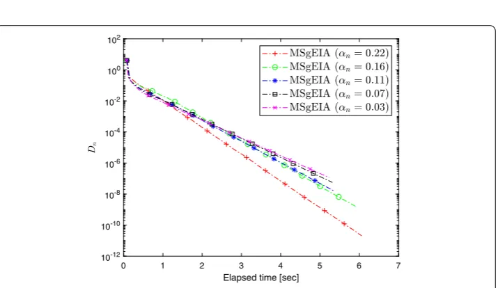
(shortly, MSgEIA) with respect to using different values ofαn. For these results, we use
pa-rametersαn= 0.22, 0.16, 0.11, 0.07, 0.03,λ0= 1 andμ= 0.11. These two figures are useful
for choosing the best possible value ofαn.
5.1.2 Algorithm2comparison with existing algorithms
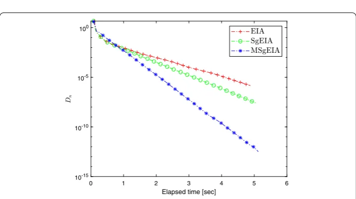
Figures3and4describe the numerical results for the first 100 iterations of Algorithm2
Al-Figure 1Experiment5.1: Algorithm2behavior in terms of iterations relative to different values ofαn
Figure 2Experiment5.1: Algorithm2behavior in terms of elapsed time relative to different values ofαn
gorithm1[Subgradient explicit iterative algorithm (shortly, SgEIA)] and explicit Algo-rithm 1 [Explicit iterative algoAlgo-rithm (shortly, EIA) [47]] in terms of no. of iterations and elapsed time in seconds.
(i) For Explicit iterative algorithm (EIA) we use the parametersμ= 0.11,λ0= 1and
Dn=xn–yn.
(ii) For Subgradient explicit iterative algorithm (SgEIA) we use the parameters
μ= 0.11,λ0= 1andDn=xn–yn.
(iii) For Modified subgradient explicit iterative algorithm (MSgEIA) we use the parametersαn= 0.12,μ= 0.11,λ0= 1andDn=wn–yn.
5.2 Nash–Cournot equilibrium models of electricity markets
[image:18.595.121.479.296.503.2]Figure 3Experiment5.1: Algorithm2comparison in terms of iterations
Figure 4Experiment5.1: Algorithm2comparison in terms of elapsed time
electricity companiesi(i= 1, 2, 3). Each companyihas its own, several generating units with index setIi. In this experiment, suppose thatI1={1},I2={2, 3}andI3={4, 5, 6}. Let
xjbe the power generation of unitsj(j= 1, . . . , 6) and suppose that the electricity pricep
can be expressed as byp= 378.4 – 26j=1xj. The cost of a generating unitjis illustrated
by
cj(xj) :=max ◦
cj(xj),
• cj(xj)
,
with
◦ cj(xj) :=
◦ αj
2x
2
j +
◦ βjxj+
[image:19.595.118.477.308.508.2]Table 1 The parameter values used in this experiment
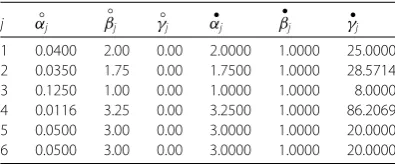
j αj◦ βj◦ γj◦ αj• βj• γj•
1 0.0400 2.00 0.00 2.0000 1.0000 25.0000 2 0.0350 1.75 0.00 1.7500 1.0000 28.5714 3 0.1250 1.00 0.00 1.0000 1.0000 8.0000 4 0.0116 3.25 0.00 3.2500 1.0000 86.2069 5 0.0500 3.00 0.00 3.0000 1.0000 20.0000 6 0.0500 3.00 0.00 3.0000 1.0000 20.0000
Table 2 The parameter values used in this experiment
j
1 2 3 4 5 6
xmin
j 0 0 0 0 0 0
xmax
j 80 80 50 55 30 40
and
• cj(xj) :=
• αjxj+
• βj
• βj+ 1
• γj
–1 •
βj(x j)
(β•j+1) •
βj ,
where the parameter values are given inα◦j,
◦ βj,
◦ γj,
• αj,
• βjand
•
γjare given in Table1. Suppose
the profit of companyiis given by
fi(x) :=p
j∈Ii
xj–
j∈Ii
cj(xj) =
378.4 – 2
6 l=1 xl
j∈Ii
xj–
j∈Ii
cj(xj),
wherex= (x1, . . . ,x6)T subject to the constraintx∈C:={x∈R6:xminj ≤xj≤xmaxj }, with
xmin j andx
max
j given in Table2.
Next, we define the equilibrium functionf by
f(x,y) :=
3
i=1
φi(x,x) –φi(x,y)
,
where
φi(x,y) :=
378.4 – 2
j∈/Ii
xj+
j∈Ii
yj j∈Ii
yj–
j∈Ii
cj(yj).
The Nash–Cournot equilibrium models of electricity markets can be reformulated as an equilibrium problem (see [58]):
Findx∗∈C such that fx∗,y≥0, ∀y∈C.
For Experiment5.2, we takex–1= (10, 0, 10, 1, 10, 1)T,x0= (48, 48, 30, 27, 18, 24)T, and
the y-axes represent for the value ofDnwhile the x-axes represent the number of iterations
Figure 5Experiment5.2: Algorithm2behavior in terms of iterations relative to different values ofλ0
Figure 6Experiment5.2: Algorithm2behavior in terms of elapsed time relative to different values ofλ0
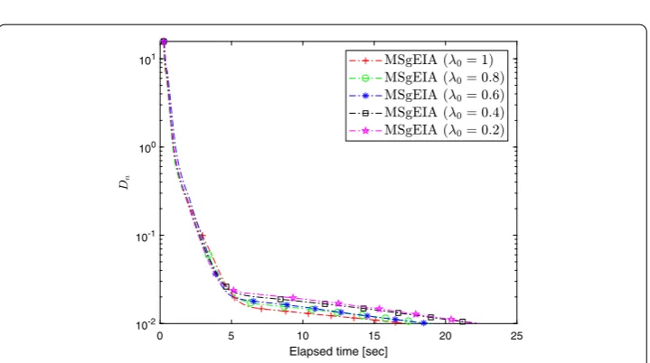
5.2.1 Algorithm2nature in terms of different values ofλ0
Figures5 and6describe the numerical results of Algorithm2 (MSgEIA) with respect to using different values of λ0, in terms of no. of iterations and elapsed time in
sec-onds relative to Dn=xn+1 –xn. For these results, we use the parameters αn= 0.20
λ0= 1, 0.8, 0.6, 0.4, 0.2,μ= 0.24 and= 10–2.
5.2.2 Algorithm2comparison with existing algorithms
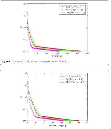
Figures7and8describe the numerical results of Algorithm2[Modified subgradient ex-plicit iterative algorithm (MSgEIA)] compared with Algorithm1[Subgradient explicit it-erative algorithm (SgEIA)] and Algorithm 1 [Explicit itit-erative algorithm (EIA) [47]] in terms of no. of iterations and elapsed time in seconds.
(i) For the Explicit iterative algorithm (EIA) we use the parametersμ= 0.2,λ0= 0.6
Figure 7Experiment5.2: Algorithm2compared in terms of iterations
Figure 8Experiment5.2: Algorithm2compared in terms of elapsed time
(ii) For Subgradient explicit iterative algorithm (SgEIA) we use the parametersμ= 0.2,
λ0= 0.6andDn=xn+1–xn.
(iii) For Modified subgradient explicit iterative algorithm (MSgEIA) we use the parametersαn= 0.20,μ= 0.2,λ0= 0.6andDn=xn+1–xn.
5.3 Two-dimensional (2-D) pseudomonotoneEP
Let us consider the following bifunction:
f(x,y) =F(x),y–x,
where
F(x) =
(x2
1+ (x2– 1)2)(1 +x2)
–x3
1–x1(x2– 1)2
withC=x∈R2: –10≤xi≤10
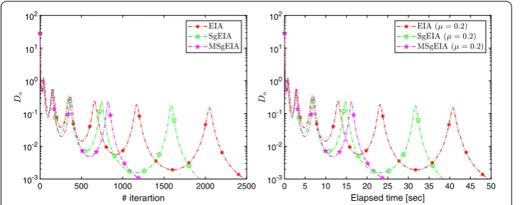
Figure 9Algorithm2compared in terms of no. of iterations and elapsed time
The bifunction is not monotone onCbut pseudomonotone (for more details see p. 10, [59,60]). Figure9illustrates the numerical results of comparison of Algorithm2with two other algorithms, withx–1= (5, 5)Tandx0= (10, 10)T.
6 Conclusion
In this paper, we propose two algorithms by incorporating the subgradient and inertial technique with an explicit iterative algorithm, which can solve the problem of a pseu-domonotone equilibrium. The evaluation of the step-size did not require a line search procedure or information on the Lipchitz-type constants of the bifunction. Rather, one uses a step-size sequence that can be updated on each iteration with the help of previous iterations. We have presented various numerical results to show the computational per-formance of our algorithm in comparison with other algorithms. These numerical results have also explained that the algorithm with inertial effects seems to perform better than without inertial effects.
Acknowledgements
The authors would like to say thanks to Professor Gabor Kassay and Auwal Bala Abubakar to providing a suggestion regarding about the Matlab program.
Funding
This project was supported by Theoretical and Computational Science (TaCS) Center under Computational and Applied Science for Smart research Innovation Cluster (CLASSIC), Faculty of Science, KMUTT. Habib ur Rehman was supported by the Petchra Pra Jom Klao Doctoral Scholarship Academic for Ph.D. Program at KMUTT (Grant No. 39/2560).
Availability of data and materials Not applicable.
Competing interests
The authors declare that they have no competing interests.
Authors’ contributions
All authors contributed equally and significantly in writing this article. All authors read and approved the final manuscript.
Author details
1Department of Mathematics, King Mongkut’s University of Technology Thonburi (KMUTT), Bangkok, Thailand.2Center
of Excellence in Theoretical and Computational Science (TaCS-CoE), SCL 802 Fixed Point Laboratory, King Mongkut’s University of Technology Thonburi (KMUTT), Bangkok, Thailand.3Department of Mathematics Education, Gyeongsang
National University, Jinju, South Korea.
Publisher’s Note
Received: 17 June 2019 Accepted: 25 October 2019 References
1. Blum, E.: From optimization and variational inequalities to equilibrium problems. Math. Stud.63, 123–145 (1994) 2. Facchinei, F., Pang, J.-S.: Finite Dimensional Variational Inequalities and Complementarity Problems. Springer, New
York (2003)
3. Konnov, I.V.: Equilibrium Models and Variational Inequalities. Elsevier, Amsterdam (2007)
4. Giannessi, F., Maugeri, A.: Variational Inequalities and Network Equilibrium Problems. Springer, New York (1995) 5. Muu, L., Oettli, W.: Convergence of an adaptive penalty scheme for finding constrained equilibria. Nonlinear Anal.,
Theory Methods Appl.18(12), 1159–1166 (1992).https://doi.org/10.1016/0362-546x(92)90159-c
6. Fan, K.: A minimax inequality and applications. In: Shisha, O. (ed.) Inequalities III. Academic Press, New York (1972) 7. Yuan, G.X.-Z.: KKM Theory and Applications in Nonlinear Analysis. CRC Press, New York (1999)
8. Brézis, H., Nirenberg, L., Stampacchia, G.: A remark on Ky Fan’s minimax principle. Boll. Unione Mat. Ital.1(2), 257–264 (2008)
9. Anh, P.N., Le Thi, H.A.: An Armijo-type method for pseudomonotone equilibrium problems and its applications. J. Glob. Optim.57(3), 803–820 (2012).https://doi.org/10.1007/s10898-012-9970-8
10. Anh, P.N., An, L.T.H.: The subgradient extragradient method extended to equilibrium problems. Optimization64(2), 225–248 (2012).https://doi.org/10.1080/02331934.2012.745528
11. Kim, J.-K., Anh, P.N., Hyun, H.-G.: A proximal point-type algorithm for pseudomonotone equilibrium problems. Bull. Korean Math. Soc.49(4), 749–759 (2012).https://doi.org/10.4134/bkms.2012.49.4.749
12. Anh, P.N., Kim, J.K.: An interior proximal cutting hyperplane method for equilibrium problems. J. Inequal. Appl.2012, Article ID 99 (2012).https://doi.org/10.1186/1029-242x-2012-99
13. Quoc, T.D., Anh, P.N., Muu, L.D.: Dual extragradient algorithms extended to equilibrium problems. J. Glob. Optim. 52(1), 139–159 (2011).https://doi.org/10.1007/s10898-011-9693-2
14. Anh, P.N., Kim, J.K.: Outer approximation algorithms for pseudomonotone equilibrium problems. Comput. Math. Appl.61(9), 2588–2595 (2011).https://doi.org/10.1016/j.camwa.2011.02.052
15. Anh, P.N., Hai, T.N., Tuan, P.M.: On ergodic algorithms for equilibrium problems. J. Glob. Optim.64(1), 179–195 (2015). https://doi.org/10.1007/s10898-015-0330-3
16. Kim, J.K., Anh, P.N., Hai, T.N.: The brucks ergodic iteration method for the Ky Fan inequality over the fixed point set. Int. J. Comput. Math.94(12), 2466–2480 (2017).https://doi.org/10.1080/00207160.2017.1283414
17. Anh, P.N., Anh, T.T.H., Hien, N.D.: Modified basic projection methods for a class of equilibrium problems. Numer. Algorithms79(1), 139–152 (2017).https://doi.org/10.1007/s11075-017-0431-9
18. Anh, P.N., Hien, N.D., Tuan, P.M.: Computational errors of the extragradient method for equilibrium problems. Bull. Malays. Math. Sci. Soc.42(5), 2835–2858 (2018).https://doi.org/10.1007/s40840-018-0632-y
19. Combettes, P.L., Hirstoaga, S.A.: Equilibrium programming in Hilbert spaces. J. Nonlinear Convex Anal.6(1), 117–136 (2005)
20. Tran, D.Q., Dung, M.L., Nguyen, V.H.: Extragradient algorithms extended to equilibrium problems. Optimization57(6), 749–776 (2008).https://doi.org/10.1080/02331930601122876
21. Moudafi, A.: Proximal point algorithm extended to equilibrium problems. J. Nat. Geom.15(1–2), 91–100 (1999) 22. Mastroeni, G.: On auxiliary principle for equilibrium problems. In: Equilibrium Problems and Variational Models.
Nonconvex Optimization and Its Applications, vol. 68, pp. 289–298. Springer, Boston (2003)
23. Martinet, B.: Régularisation d’inéquations variationnelles par approximations successives. Rev. Fr. Inform. Rech. Oper. 4(R3), 154–158 (1970).https://doi.org/10.1051/m2an/197004r301541
24. Rockafellar, R.T.: Monotone operators and the proximal point algorithm. SIAM J. Control Optim.14(5), 877–898 (1976). https://doi.org/10.1137/0314056
25. Cohen, G.: Auxiliary problem principle and decomposition of optimization problems. J. Optim. Theory Appl.32(3), 277–305 (1980).https://doi.org/10.1007/bf00934554
26. Cohen, G.: Auxiliary problem principle extended to variational inequalities. J. Optim. Theory Appl.59(2), 325–333 (1988).https://doi.org/10.1007/bf00938316
27. Korpelevich, G.: The extragradient method for finding saddle points and other problems. Matecon12, 747–756 (1976)
28. Censor, Y., Gibali, A., Reich, S.: The subgradient extragradient method for solving variational inequalities in Hilbert space. J. Optim. Theory Appl.148(2), 318–335 (2010).https://doi.org/10.1007/s10957-010-9757-3
29. Popov, L.D.: A modification of the Arrow–Hurwicz method for search of saddle points. Math. Notes Acad. Sci. USSR 28(5), 845–848 (1980).https://doi.org/10.1007/bf01141092
30. Tseng, P.: A modified forward–backward splitting method for maximal monotone mappings. SIAM J. Control Optim. 38(2), 431–446 (2000).https://doi.org/10.1137/s0363012998338806
31. He, B.: A class of projection and contraction methods for monotone variational inequalities. Appl. Math. Optim.35(1), 69–76 (1997).https://doi.org/10.1007/bf02683320
32. Yamada, I.: The hybrid steepest descent method for the variational inequality problem over the intersection of fixed point sets of nonexpansive mappings. Stud. Comput. Math.8, 473–504 (2001).
https://doi.org/10.1016/s1570-579x(01)80028-8
33. Xu, H.K., Kim, T.H.: Convergence of hybrid steepest-descent methods for variational inequalities. J. Optim. Theory Appl.119(1), 185–201 (2003).https://doi.org/10.1023/b:jota.0000005048.79379.b6
34. Bertsekas, D.P., Gafni, E.M.: Projection methods for variational inequalities with application to the traffic assignment problem. In: Mathematical Programming Studies, pp. 139–159. Springer, Berlin (1982).
https://doi.org/10.1007/bfb0120965
35. Zhu, M., Chan, T.: An efficient primal-dual hybrid gradient algorithm for total variation image restoration. UCLA CAM report 34 (2008)
36. Flåm, S.D., Antipin, A.S.: Equilibrium programming using proximal-like algorithms. Math. Program.78(1), 29–41 (1996). https://doi.org/10.1007/bf02614504
38. Kassay, G., Hai, T.N., Vinh, N.T.: Coupling Popov’s algorithm with subgradient extragradient method for solving equilibrium problems. J. Nonlinear Convex Anal.19(6), 959–986 (2018)
39. Liu, Y., Kong, H.: The new extragradient method extended to equilibrium problems. Rev. R. Acad. Cienc. Exactas Fís. Nat., Ser. A Mat. (2018).https://doi.org/10.1007/s13398-018-0604-y
40. Polyak, B.T.: Some methods of speeding up the convergence of iteration methods. USSR Comput. Math. Math. Phys. 4, 1–17 (1964).https://doi.org/10.1016/0041-5553(64)90137-5
41. Beck, A., Teboulle M.: A fast iterative shrinkage-thresholding algorithm for linear inverse problems. SIAM J. Imaging Sci.2, 183–202 (2009).https://doi.org/10.1137/080716542
42. Dong, Q.-L., Lu, Y.-Y., Yang, J.: The extragradient algorithm with inertial effects for solving the variational inequality. Optimization65, 2217–2226 (2016).https://doi.org/10.1080/02331934.2016.1239266
43. Bo¸t, R.I., Csetnek, E.R., László, S.C.: An inertial forward–backward algorithm for the minimization of the sum of two nonconvex functions. EURO J. Comput. Optim.4, 3–25 (2016).https://doi.org/10.1007/s13675-015-0045-8 44. Maingé, P.-E., Moudafi, A.: Convergence of new inertial proximal methods for DC programming. SIAM J. Optim.19,
397–413 (2008).https://doi.org/10.1137/060655183
45. Moudafi, A.: Second-order differential proximal methods for equilibrium problems. J. Inequal. Pure Appl. Math.4(1), 1–7 (2003)
46. Chbani, Z., Riahi, H.: Weak and strong convergence of an inertial proximal method for solving Ky Fan minimax inequalities. Optim. Lett.7, 185–206 (2013).https://doi.org/10.1007/s11590-011-0407-y
47. Van Hieu, D., Quy, P.K., Van Vy, L.: Explicit iterative algorithms for solving equilibrium problems. Calcolo56, Article ID 11 (2019).https://doi.org/10.1007/s10092-019-0308-5
48. Van Hieu, D.: An inertial-like proximal algorithm for equilibrium problems. Math. Methods Oper. Res.88, 399–415 (2018).https://doi.org/10.1007/s00186-018-0640-6
49. Van Hieu, D.: New inertial algorithm for a class of equilibrium problems. Numer. Algorithms80, 1413–1436 (2019). https://doi.org/10.1007/s11075-018-0532-0
50. Goebel, K., Reich, S.: Uniform Convexity, Hyperbolic Geometry, and Nonexpansive Mappings. Dekker, New York (1984) 51. Kreyszig, E.: Introductory Functional Analysis with Applications. Wiley, New York (1978)
52. Bianchi, M., Schaible, S.: Generalized monotone bifunctions and equilibrium problems. J. Optim. Theory Appl.90, 31–43 (1996).https://doi.org/10.1007/bf02192244
53. Hieua, D.V.: Parallel extragradient-proximal methods for split equilibrium problems. Math. Model. Anal.21, 478–501 (2016).https://doi.org/10.3846/13926292.2016.1183527
54. van Tiel, J.: Convex Analysis: An Introductory Text, 1st edn. Wiley, New York (1984)
55. Bauschke, H.H., Combettes, P.L.: Convex Analysis and Monotone Operator Theory in Hilbert Spaces. Springer, New York (2011)
56. Alvarez, F., Attouch, H.: An inertial proximal method for maximal monotone operators via discretization of a nonlinear oscillator with damping. Set-Valued Var. Anal.9, 3–11 (2001).https://doi.org/10.1023/a:1011253113155
57. Opial, Z.: Weak convergence of the sequence of successive approximations for nonexpansive mappings. Bull. Am. Math. Soc.73, 591–598 (1967).https://doi.org/10.1090/S0002-9904-1967-11761-0
58. Konnov, I.: Combined Relaxation Methods for Variational Inequalities. Lecture Notes in Economics and Mathematical Systems, vol. 495. Springer, New York (2001)
59. Hu, X., Wang, J.: Solving pseudomonotone variational inequalities and pseudoconvex optimization problems using the projection neural network. IEEE Trans. Neural Netw.17, 1487–1499 (2006).
https://doi.org/10.1109/TNN.2006.879774