Quantitative characterization of 3D deformations of cell interactions with soft biomaterials

(1)

Quantitative Characterization of 3D Deformations of Cell

Interactions with Soft Biomaterials

Thesis by

Christian Franck

In Partial Fulfillment of the Requirements for the Degree of

Doctor of Philosophy

California Institute of Technology Pasadena, California

2008

(2)

c

2008

(3)

iii

(4)

Acknowledgments

I would like to begin by thanking all of my friends whom I have interacted with over the course of my five years here at Caltech. Your friendship, interactions and discussions have made my experience at Caltech truly rewarding, enriching and wonderful. In particular, I would like to thank some outstanding individuals who have made my personal and academic adventures at Caltech particularly special. Foremost, I want to thank my advisor Professor Ravichandran who besides many things taught me that nothing is ever impossible no matter how insurmountable the task may seem. I would like to thank him for making all my endeavors possible and providing me with so many wonderful opportunities, for that I am truly grateful.

(5)

v

night. I want to thank Linda Miranda not only for being the best assistant ever, but also for many funny and joyful conversations including random trips to the bookstore and the post office. I want to gratefully acknowledge the funding support for this project sponsored by the National Science Foundation through their Materials Research Science and Engineering Center at Caltech. I would like to thank Winston Jackson for his friendship and all the great discussions both academically and personally during my time at Caltech.

(6)

Abstract

In recent years, the importance of mechanical forces in directing cellular function has been recognized as a significant factor in biological and physiological processes. In fact, these physical forces are now viewed equally as important as biochemical stimuli in controlling cellular response. Not only do these cellular forces, or cell tractions, play an important role in cell migration, they are also significant to many other physiological and pathological processes, both at the tissue and organ level, including wound healing, inflammation, angiogenesis, and embryogenesis. A complete quantification of cell tractions during cell-material interactions can lead to a deeper understanding of the fundamental role these forces play in cell biology. Thus, understanding the function and role of a cell from a mechanical framework can have important implications towards the development of new implant materials and drug treatments.

(7)

ex-vii

ternally applied deformations. This method is validated by comparing experimentally measured non-uniform deformation fields near hard and soft spherical inclusions under uniaxial compression with the corresponding analytical solution. Utilization of a newly developed computationally effi-cient stretch-correlation and deconvolution algorithm is shown to improve the overall measurement accuracy, in particular under large deformations.

Using this technique, the full three-dimensional substrate displacement fields are experimentally determined during the migration of individual fibroblast cells on polyacrylamide gels. This is the first study to show the highly three-dimensional structure of cell-induced displacement and traction fields. These new findings suggest a three-dimensional push-pull cell motility, which differs from the traditional theories based on two-dimensional data. These results provide new insight into the dynamic cell-matrix force exchange or mechanotransduction of migrating cells, and will aid in the development of new three-dimensional cell motility and adhesion models.

(8)

List of Figures

2.1 Illustration of the confocal imaging principle (solid lines = in-focus light; dashed lines

= out-of-focus light) . . . 11 2.2 Profiles of the PSF for u= 0 (lateral), and v = 0 (vertical) from Stevenset al. [47].

The units ofuand vare arbitrary optical units (ou). The peak widths determine the

resolution.. . . 12 2.3 Isosurface plot of fluorescent particles as recorded by LSCM (1 voxel = 0.45µm) . . . 15 2.4 Isosurface plot of fluorescent particles after deconvolution of the PSF (1 voxel = 0.45

µm) . . . 15 2.5 Schematic illustration of the principle of digital volume correlation (DVC). . . 16 2.6 Ilustration of the stretch-correlation procedures using a one-dimensional (1D) example 20 2.7 Two-dimensional projection of confocal subvolume images (a) before and (b) after

uniaxial compression of 10% inx3-direction . . . 21

2.8 Loading fixture for uniaxial compression of soft materials mounted onto a laser scanning

confocal microscope . . . 23 2.9 Experimentally determined three-dimensional displacement vector field under uniaxial

compression. . . 25 2.10 Experimentally determined vertical displacement fieldu3 under uniaxial compression. 25

2.11 Schematic of a spherical inclusion with a sliding interface under confined uniaxial

com-pression . . . 27 2.12 Confocal slice along the meridian plane of an embedded 100 µm PMMA bead within

(12)

2.13 Confocal slice along the meridian plane of an embedded 200 µm air bubble within an

agarose sample . . . 30 2.14 Cross-section of the experimentally determined vertical displacement field u3 near

PMMA bead inclusion under uniaxial compression. Contour values are in pixels (1

pixel = 0.45µm). . . 32 2.15 Cross-section of the experimentally determined vertical displacement fieldu3 near air

bubble inclusion under uniaxial compression. Contour values are in pixels (1 pixel =

0.45µm). . . 32 2.16 Cross-section of the stretch-corrected measured vertical displacement fieldu3near the

PMMA bead inclusion under uniaxial compression. Contour values are in pixels (1

pixel = 0.45µm). . . 32 2.17 Cross-section of the stretch-corrected measured vertical displacement fieldu3near the

air bubble inclusion under uniaxial compression. Contour values are in pixels (1 pixel

= 0.45µm).. . . 32 2.18 Experimentally determined vertical displacement field u3 near PMMA bead inclusion

under uniaxial compression. Contour values are in pixels (1 pixel = 0.45µm). . . 33 2.19 Experimentally determined vertical displacement field u3 near air bubble inclusion

under uniaxial compression. Contour values are in pixels (1 pixel = 0.45µm). . . 33 2.20 Analytical vertical displacement field u3 near a rigid bead inclusion with a sliding

interface under uniaxial constrained compression. Contour values are in pixels (1 pixel

= 0.45µm).. . . 33 2.21 Analytical vertical displacement field u3 near a soft inclusion with a sliding interface

under uniaxial constrained compression. Contour values are in pixels (1 pixel = 0.45

µm). . . 33 2.22 Experimentally determined vertical strain field33near a PMMA bead inclusion under

(13)

xiii

2.23 Experimentally determined vertical strain field33 near an air bubble inclusion under

uniaxial compression . . . 34 2.24 Plot of the experimentally determined strain field33as a function of outward distance

(x3 = 0 denotes the center of the inclusion) in the meridian plane of the spherical

PMMA inclusion under uniaxial compression . . . 35

3.1 Representative force history plot during uniaxial compression experiments on a

poly-acrylamide gel showing negligible time-dependent material behavior. . . 42 3.2 Representative loading and unloading stress-strain plot of a polyacrylamide gel,

high-lighting the linear elastic material response with negligible hysteresis. . . 42

4.1 Surface contour plots of the magnitude of the three-dimensional displacement vector

during cell migration. The color bar represents the magnitude of the total

three-dimensional displacement vectors inµm, and the cell (green) is superimposed on the

three-dimensional contour plots to show its position with respect to the deformation

field.. . . 49 4.2 Arbitrary displacement contour slices along the long axis of the cell. The slices of

displacement contours underneath migrating cells show significant deformation in the

normal plane that decay along the thickness of the sample. The two edges in the image

are included to show that there are negligible displacements detected from neighboring

cells (contours are dark blue). The color bar represents the magnitude of the total

three-dimensional displacement vectors inµm, and the cell (green) is superimposed on

the three-dimensional contour plots to show its position with respect to the deformation

(14)

4.3 Displacement contour and line plot profiles as a function of depth (x3) through the

thickness of the gel. Figure 4.3(a) shows the same displacement contours along the long

axis of the cell as shown in Fig. 4.2(a), where the color bar represents the magnitude

of the three-dimensional displacement vectors inµm, and the white arrows show the

direction of the in-plane (u1,u3) displacement components only. Figure 4.3(b) shows

the zoom-in image of Fig. 4.3(a), whereas Fig. 4.3(c) illustrates the decay of all three

displacement components in thex3 direction, wherex3= 14 represents the location of

the top surface.. . . 52 4.4 Displacement contour and line plot profiles as a function of depth (x3) through the

axis of the cell as shown in Fig. 4.2(b), where the color bar represents the magnitude

displacement components in thex3 direction, wherex3= 14 represents the location of

the top surface.. . . 53 4.5 Surface displacement contour and line plot profiles along a particular line in thex1−x2

surface plane att1 = 35 min. Figure 4.5(a) shows the same displacement contours as

shown in Fig. 4.1(a), where the color bar represents the magnitude of the

three-dimensional displacement vectors inµm, and the white arrows show the direction of

the in-plane (u1,u2) displacement components only. Figure 4.5(b) shows the zoom-in

image of Fig. 4.5(a) highlighting the particular region where the line plot was generated.

Figure 4.5(c) illustrates the distribution of all three displacement components along the

(15)

xv

4.6 Surface displacement contour and line plot profiles along a particular line in thex1−x2

surface plane att2 = 70 min. Figure 4.6(a) shows the same displacement contours as

shown in Fig. 4.1(b), where the color bar represents the magnitude of the

three-dimensional displacement vectors inµm, and the white arrows show the direction of

the in-plane (u1,u2) displacement components only. Figure 4.5(b) shows the zoom-in

image of Fig. 4.6(a) highlighting the particular region where the line plot was generated.

Figure 4.6(c) illustrates the distribution of all three displacement components along the

selected line. . . 56 4.7 Comparison between the displacement magnitude of all three-dimensional vector

com-ponents (4.7(a) and 4.7(c)) and the magnitude of the two-dimensional vector

compo-nents only (4.7(b) and 4.7(d)). The color bar is displaying all displacement values

µm, and and the white arrows show the direction of the in-plane (u1,u2) displacement

components only. . . 57 4.8 Surface contour plots of the magnitude of the three-dimensional traction vector during

cell migration. The color bar represents the magnitude of the total three-dimensional

surface traction vectors inpN/µm2_{, and the cell (green) is superimposed on the}

three-dimensional contour plots to show its position with respect to the traction field. . . . 59 4.9 Arbitrary traction contour slices along the long axis of the cell. The color bar indicates

the magnitude of the three-dimensional traction vectors along that particular plane in

units of pN/µm2. The slices of the traction contours underneath the migrating cells correspond to the displacement slices shown in Fig. 4.2. The two edges in the image

are included to show that there are negligible tractions detected from neighboring cells

(contours are dark blue). The cell (green) is superimposed on the three-dimensional

(16)

4.10 Traction contour and line plot profiles as a function of depth (x3) through the thickness

of the gel at timet1 = 35 min. Figure 4.10(a) shows the same traction contours along

the long axis of the cell as shown in Fig. 4.9(a), where the color bar represents the

magnitude of the three-dimensional traction vectors along that particular plane, and

the white arrows show the direction of the in-plane (T1,T3) traction components only.

Figure 4.10(b) shows the zoom-in image of Fig. 4.10(a), whereas Fig. 4.10(c) illustrates

the decay of all traction components and the magnitude of the three-dimensional

trac-tion vector in thex3 direction. The color bar units are displayed inpN/µm2. . . 62

the long axis of the cell as shown in Fig. 4.9(b), where the color bar represents the

trac-tion vector in thex3 direction. The color bar units are displayed inpN/µm2. . . 63

4.12 Surface tractions contour and line plot profiles along a particular line in thex1−x2top

surface plane att1= 35 min. Figure 4.12(a) shows the same traction contours as shown

in Fig. 4.8(a), where the color bar represents the magnitude of the three-dimensional

surface traction vectors and the white arrows show the direction of the in-plane (T1,T2)

traction components only. The color bar units are inpN/µm2. Figure 4.5(b) shows the zoom-in image of Fig. 4.12(a) highlighting the particular region, where the line plot was

generated. Figure 4.12(c) illustrates the distribution of all three traction components

(17)

xvii

4.13 Surface traction contour and line plot profiles along a particular line in thex1−x2top

surface plane at t2 = 70 min. Figure 4.13(a) shows the same traction force contours

as shown in Fig. 4.8(b), where the color bar represents the magnitude of the

three-dimensional surface traction vectors and the white arrows show the direction of the

in-plane (T1,T2) traction components only. The color bar units arepN/µm2. Figure

4.6(b) shows the zoom-in image of Fig. 4.13(a) highlighting the particular region,

where the line plot was generated. Figure 4.13(c) illustrates the distribution of all

three traction components and the magnitude of the three-dimensional traction vector

along the drawn line. . . 66 4.14 Comparison between the magnitude of the three-dimensional traction vector (4.14(a)

and 4.14(c)) and the magnitude of the two-dimensional traction vector (T1, T2)

com-ponents only (4.14(b) and 4.14(d))). The color bar is displaying all traction values in

pN/µm2, and and the white arrows show the direction of the in-plane (T1,T2) traction

components only. . . 67 4.15 Surface contour plots of the magnitude of the three-dimensional displacment vector

during cell migration. The color bar represents the magnitude of the total

three-dimensional displacement vectors inµm, and the cell (green) is superimposed on the

three-dimensional contour plots to show its position with respect to the deformation

field.. . . 69 4.16 Arbitrary displacement contour slices along the long axis of the cell. The slices of

displacement contours underneath migrating cells show significant deformation in the

normal plane that decay along the thickness of the sample. The two edges in the image

are included to show that there are negligible displacements detected from neighboring

cells (contours are dark blue). The color bar represents the magnitude of the total

three-dimensional displacement vectors inµm, and the cell (green) is superimposed on

the three-dimensional contour plots to show its position with respect to the deformation

(18)

axis of the cell as shown in Fig. 4.16(a), where the color bar represents the magnitude

displacement components and the magnitude of the three-dimensional displacement

vector in thex3 direction. . . 71

thickness of the gel. Part 4.18(a) shows the same displacement contours along the long

axis of the cell as shown in Fig. 4.16(b), where the color bar represents the magnitude

displacement components and the magnitude of the three-dimensional displacement

vector in thex3 direction. . . 73

4.19 Surface displacement contour and line plot profiles along a particular line in thex1−

x2 top surface plane at t1 = 35 min. Figure 4.19(a) shows the same displacement

contours as shown in Fig. 4.15(a), where the color bar represents the magnitude of

the three-dimensional displacement vectors in µm, and the white arrows show the

the zoom-in image of Fig. 4.19(a) highlighting the particular region, where the line

plot was generated. Figure 4.19(c) illustrates the distribution of all three displacement

components and the magnitude of the three-dimensional displacement vector along the

(19)

xix

4.20 Surface displacement contour and line plot profiles along a particular line in thex1−

x2 top surface plane at t2 = 70 min. Figure 4.20(a) shows the same displacement

contours as shown in Fig. 4.15(b), where the color bar represents the magnitude of

the three-dimensional displacement vectors in µm, and the white arrows show the

the zoom-in image of Fig. 4.20(a) highlighting the particular region, where the line

plot was generated. Figure 4.20(c) illustrates the distribution of all three displacement

components and the magnitude of the three-dimensional displacement vector along the

drawn line. . . 76 4.21 Comparison between the displacement magnitude of all three-dimensional vector

com-ponents (4.21(a) and 4.21(c)) and the magnitude of the two-dimensional vector

compo-nents only (4.21(b) and 4.21(d)). The color bar is displaying all displacement values in

µm, and and the white arrows show the direction of the in-plane (u1,u2) displacement

components only. . . 77 4.22 Surface contour plots of the magnitude of the three-dimensional traction vector during

cell migration. The color bar represents the magnitude of the total three-dimensional

surface traction vectors with units inpN/µm2_{, and the cell (green) is superimposed on}

the three-dimensional contour plots to show its position with respect to the traction

field.. . . 78 4.23 Arbitrary traction contour slices along the long axis of the cell. The color bar indicates

the magnitude of the three-dimensional traction vectors along that particular plane

in units of pN/µm2_{. The slices of the traction contours underneath migrating cells}

correspond to the displacement slices shown in Fig. 4.16. The two edges in the image

are included to show that there are negligible tractions detected from neighboring cells

(contours are dark blue). The cell (green) is superimposed on the three-dimensional

(20)

the long axis of the cell as shown in Fig. 4.23(a), where the color bar represents the

trac-tion vector in thex3 direction. All color bar units arepN/µm2. . . 81

the long axis of the cell as shown in Fig. 4.23(b), where the color bar represents the

trac-tion vector in thex3 direction. All color bar units arepN/µm2. . . 82

4.26 Surface traction contour and line plot profiles along a particular line in the x1−x2

top surface plane at t1 = 35 min. Figure 4.26(a) shows the same traction contours

as shown in Fig. 4.22(a), where the color bar represents the magnitude of the

in-plane (T1,T2) traction components only. The color bar units represent pN/µm2.

Figure 4.19(b) shows the zoom-in image of Fig. 4.26(a) highlighting the particular

region, where the line plot was generated. Figure 4.26(c) illustrates the distribution

of all three traction components and the magnitude of the three-dimensional traction

(21)

xxi

4.27 Surface traction contour and line plot profiles along a particular line in the x1−x2

surface plane at t2 = 70 min. Figure 4.27(a) shows the same traction contours as

shown in Fig. 4.22(b), where the color bar represents the magnitude of the

in-plane (T1,T2) traction components only. The color bar units represent pN/µm2.

Figure 4.6(b) shows the zoom-in image of Fig. 4.27(a) highlighting the particular

region, where the line plot was generated. Figure 4.27(c) illustrates the distribution

of all three traction components and the magnitude of the three-dimensional traction

vector along the drawn line.. . . 85 4.28 Comparison between the magnitude of the three-dimensional traction vector (4.28(a)

and 4.28(c) and the magnitude of the two-dimensional traction vector (T1, T2)

com-ponents only (4.28(b) and 4.28(d))). The color bar is displaying all traction values in

pN/µm2, and and the white arrows show the direction of the in-plane (T1,T2) traction

components only. . . 86 4.29 Successive time series of cell-induced surface displacements before (4.29(a) and 4.29(b))

and after treatment with blebbistatin (4.29(c) and 4.29(d)). Color contours display the

magnitude of the three-dimensional displacement vector, while the white arrows show

the direction of the in-plane (u1,u2) displacement components only. The color bar

represents all values inµm. . . 88 4.30 Comparison between the three-dimensional cell induced surface deformation on soft

(4.31(a) and 4.31(b)) andstiff (4.31(c) and 4.31(d)) polyacrylamide gel substrates for

a 35 min time increment. The color bar in Figs. 4.31(a) and 4.31(c) indicates all

values inµm, whereas the color bar in Figs. 4.31(b) and 4.31(d) displays all values in

pN/µm2_{. The Young’s moduli of the}_soft _and_stiff _{substrates are 0.82 and 9.64 kPa,}

(22)

4.31 Comparison between the three-dimensional cell induced surface deformation on soft

(4.31(a) and 4.31(b)) andstiff (4.31(c) and 4.31(d)) polyacrylamide gel substrates for

a 35 min time increment. The color bar in Figs. 4.31(a) and 4.31(c) indicates all values

inµm, whereas the color bar in Figs. 4.31(b) and 4.31(d) displays all measurements in

pN/µm2. The Young’s moduli of thesoft andstiff substrates are 0.82 and 9.64 kPa, respectively. . . 91 4.32 A schematic of the four basic steps involved in cell motion. Movement is initiated

by the protrusion of the the cystoskeleton by actin polymerization 4.32(a) followed by

formation of focal adhesion complexes and adhesion to the substrate 4.32(b). Next,

the cell detaches its trailing edge from the substrate 4.32(c) and finally generates an

internal force to contract and propel itself forward 4.32(d). . . 94 4.33 Time evolution of cell-induced tractions as a function of depth (x3) over 70 min along

an arbitrary slice below the cell’s long axis. The contour plots show the magnitude of

the three-dimensional traction vector as previously plotted in Figs. 4.24(a) - 4.25(a).

The black arrows represent the in-plane shear tractions (T1,T3), where the magnitude

of the longest arrow in each Fig. is equal to the maximum value depicted by the color

bar inpN/µm2_{. The particular time increments that are shown here are}_t

2,t3, andt4,

where the time increment between each frame is 35 min. The leading edge of the cell

is located on the right (∼x1 = 120 µm), and the direction of cell migration is from

(23)

xxiii

4.34 Time evolution of cell-induced shear tractions (T1,T3) as a function of depth (x3) over

70 min along an arbitrary slice below the cell’s long axis. The contour plots show

the magnitude of the shear traction components (left column: T3; right column: T1).

The color bar units arepN/µm2_{. The black arrows on the top of each plot give the}

general direction of the cell-generated tractions. The particular time increments that

are shown here aret2, t3, andt4, where the time increment between each frame is 35

min. The leading edge of the cell is located on the right (∼ x1 = 120µm), and the

direction of cell migration is from left to right. . . 96

5.1 LSCM image depicting three arbitrary planar slices of the entire volumetric image stack

at two different imaging times. Fibroblast cells displaying GFP-actin are shown in red,

whereas the 0.5µm fluorescent microspheres are shown in yellow. . . 100 5.2 Time series of the LSCM-DVC measured three-dimensional displacement vector fields.

The average vector length in each plot is between 0.06 - 0.18µm. The fibroblasts cells

are superimposed in green (GFP-actin). . . 101

A.1 Amino acid sequence of the artificial extracellular matrix protein examined in this work.

The cell-binding sequence CS5 is underlined. Proteins containing the photosensitive

amino acid para-azidophenylalanine are designated aE-pN3Phe.. . . 106

A.2 AFM topography scans of cut edges of an aE-48%-pN3Phe film, dry (A) and in water

(B). The spikes at the edge are artifacts of the scratching procedure. . . 107 A.3 Representative loading indentation profiles for thin films of aE-66%-pN3Phe and

aE-48%-pN3Phe, showing force versus indentation depth (z-displacement). (A) shows the

entire profiles; (B) is magnified to show the contact point assignment. . . 109 A.4 (A) Superimposed force profiles for multiple indentations of a single aE-48%-pN3Phe

film for 1 sec and 10 sec indent cycles. (B) Calculated Young’s modulus for 1 sec and

(24)

A.5 The elastic modulus (E) calculated at each point in the AFM indentation using Hertz

and Dimitriadis models (Eq. A.1) is shown for an aE-48%-pN3Phe film. . . 115

A.6 Experimental AFM indentation data compared to Dimitriadis model (Eq. A.1) fits for

thin films of aE-66%-pN3Phe and aE-48%-pN3Phe. . . 115

A.7 Superposition of experimental AFM data and finite element simulations of indentation

based on bulk tensile data for thin films of aE-66%-pN3Phe and aE-48%-pN3Phe. . . 116

A.8 Sample tensile data for bulk films containing varying amounts ofpN3Phe. . . 116

A.9 Measured elastic moduli of thin films of aE-pN3Phe versus fraction replacement of Phe

by pN3Phe. Results from AFM nanoindentation of thin films and tensile testing of

bulk films are compared. . . 119 A.10 Preparation of a step gradient in elastic modulus by variable irradiation of a single

aE-66%-pN3Phe film. Error bars indicate standard deviation in modulus within each

(25)

xxv

List of Tables

2.1 Standard deviation values for measured displacement and strain fields in the

unde-formed condition . . . 24 2.2 Mean and standard deviation values for measured strain fields under uniaxial compression 26

3.1 Young’s modulus values for polyacrylamide substrates with different crosslinker volume

fraction. . . 42 3.2 Standard deviation values for measured displacement fields in the undeformed condition

for agarose gels at 25o C and polyacrylamide gels at 37o C . . . 44

A.1 Expression conditions and protein yields. . . 111 A.2 Physical properties of bulk aE-pN3Phe films tested in uniaxial tension (n=2). . . 114

(26)

Chapter 1

Introduction

1.1 Mechanics in the Context of Cell Biology

Mechanical forces play an important role in the activities of our daily lives from sitting to lifting objects to running. During all of these activities our bones and ligaments experience cycles of different mechanical loads, and need to adjust accordingly. For example, a runner’s foot constantly experiences physical forces as it periodically impacts the ground. These forces are balanced by the runner’s joints and bones, where the bone carries some of the compressive loading. If we examine the structure of the runner’s bone in more detail, we would find a fairly porous structure made up of mostly calcium phosphate and collagen fibers, much resembling a light-weight composite structure. Intertwined with this structure are cells, some of which are constantly remodeling and restructuring the bone adjusting to the external loading.

In fact, one can think of the bone as an active mechanical system in which a particular type of cells called osteocytes act as mechanosensors. These “sensor” cells can communicate with other cells through an intricate feedback system to ensure the health or homeostasis of the bone itself. In particular, two of the cells with which osteocytes communicate are osteoblasts and osteoclasts. Osteoblasts are responsible for bone remodeling or remineralization. Osteoclasts, on the other hand, are in charge of removing or resorbing bone. So, in order to maintain a healthy bone structure, the activities of osteoblasts and osteoclasts need to be balanced.

(27)

2

loading were to be removed, as in the case of an astronaut in space (zero-gravity environment), then the osteoblasts will cease to create more healthy bone structure due to the absence of the mechanical stimulus. Another type of imbalance is created in the case of osteoporosis, where insufficient os-teoblasts exist to counteract the bone removal created by the more numerous osteoclasts. Of course this is a simplification of a delicate biochemical and mechanical system, which needs to be fully understood in order to maintain healthy, long-lasting bones.

Another example of the importance mechanical forces play in cellular behavior, is when tumor cells metastasize, or spread to the surrounding tissue in the body. In this case, as the tumor cells spread from their primary site they must venture through a jungle of extracellular proteins, such as proteoglycans, collagen, and elastin fibers collectively known as the extracellular matrix (ECM). For these malignant cells to successfully reach the arterial walls they need to push, squeeze, and cleave their way through the ECM, which involves exerting mechanical forces. Yet unfortunately, this migration mechanism, in particular the three-dimensional cell-matrix force exchange is relatively poorly understood.

As suggested by the above examples, there is an established connection between mechanical forces and cellular function [45]. In fact, these physical forces are today viewed equally as impor-tant as biochemical stimuli in directing cellular response. The translation of mechanical forces into biochemical signals that are responsible for determining cellular behavior is coined mechanotrans-duction [23]. Since the purpose of this investigation focuses on the physical interactions of cells and their ECM, the following overview presents a rather simplified version of the intricate interplay between mechanical forces and biochemical signaling, which can be found in more detail elsewhere [7,24,29,36].

(28)

these forces to take place, the cell needs to anchor itself to the surrounding ECM. These particular anchor points that connect the cell to the ECM are called focal adhesion sites. They serve as a gateway for the cell to transmit its internal forces to the ECM and vice versa.

Internal cellular forces are created through the interaction of actin with myosin II. Actin is one of the three structural elements found inside the cell, beside microtubules and intermediate filaments. Actin filaments can form long bundles also known as stress fibers that form a collaborate intracellular network that connects the focal adhesion sites (e.g., α and β integrins), much like truss structures support a steel bridge. Myosin II is a molecular motor protein that hydrolizes adenosine-50-triphosphate (ATP) for energy, and induces contraction of the actin framework. The cell membrane has receptors or integrins that connect to the ECM proteins or ligands at the focal adhesion site. Cell contraction is first felt by actin, then transmitted to the membrane receptors across a multitude of focal adhesion proteins and finally to the ECM ligands. In order for the cell to move, all it needs to do is to detach from a particular focal adhesion site, thus creating a force imbalance. Not only do these cellular forces or cell traction forces play an important role in cell migration, they are also significant to many other physiological and pathological processes, both at the tissue and organ level. Some of these include wound healing, inflammation, angiogenesis, and embryogenesis [54]. Hence, quantification and understanding of their nature and regulation become an important part for the development of new implant material and drug treatments.

1.2 Previous Work on Quantifying Cell-ECM Interactions

(29)

4

substrate surfaces [13,34,27]. This method utilizes optical phase and wide-field microscopy to track substrate surface displacements due to cellular traction forces via fluorescent particles embedded in a polyacrylamide substrate. This technique is currently one of the most widely used methods in determining cellular traction forces that are part of the mechanotransduction process. It will be described in more detail within the next section.

Another method to determine cell-induced traction forces was proposed by Tan et al. in 2003 where, instead of using fluorescent beads, thin cantilevers (micro needle-like posts) are fabricated out of poly-dimethylsiloxane (PDMS) substrates, from which traction forces can be calculated according to linear beam theory [49]. This method produces similar spatial resolution as the TFM technique on the micrometer scale with resolved forces of the order of nano-Newtons. Yet another approach demonstrated by Balabanet al. relies on displacement measurements of submicron patterned dots on PDMS susbtrate. However, both this technique and TFM employ an inverse Bousinessq formulation to convert the observed displacements into traction forces as will be explained later. Although these reports have contributed much to describing cell behaviors in two-dimensional environments, many physiological processes are three dimensional in nature and recent studies have not only shown morphological differences in cells cultured on two-dimensional substrates versus three-dimensional matrices, but their intrinsic ECM interactions and migration behavior also appears different [12,16, 55]. Yet few advances have been made to address the need for three-dimensional quantitative imaging techniques [32]. Thus, a new class of experimental tools capable of quantitatively capturing such interactions is needed for more in-depth studies. This thesis presents a three-dimensional imaging technique capable of quantitatively measuring cell traction forces in all three spatial dimensions.

1.2.1 Traction Force Microscopy (TFM)

(30)

poly-acrylamide or similar polymer based substrates with typical Young’s moduli ranging from∼1 - 30 kPa [14,7,38]. Balaban et al. used a geometrical pattern stamped into PDMS to track cell-induced surface displacements. To record cell surface deformations, cells are initially seeded on the substrate material and allowed to spread and migrate. After some time, a first image is recorded via an opti-cal microscope, where typiopti-cally both the cell and the tracker particles are recorded simultaneously. Then, the cells are chemically detached from the surface involving cleaving proteases such as trypsin to disrupt all cell substrate attachments. Without moving the microscope objective another image is captured serving as the undeformed or reference configuration. The two-dimensional full-field displacements are then determined from the set of the two images by either using a single particle tracking or digital image correlation algorithm.

In order to determine the cell-induced surface traction forces from the recorded displacement data, the Boussinesq formulation is utilized. The Boussinesq theory describes the displacement equilibrium solutions inside a semi-infinite elastic half-space with applied forces at its free boundary (surface) via the governing equation

∇(∇ ·u(x)) + (1−2ν)∇2_u₍_x_{) = 0} _(1.1)

whereu(x) is the three-dimensional displacement vector, andν is the Poisson’s ratio of the linearly elastic material. The details of the derivation in formulating the solution is given by Landau and Lifshitz [25], so only the end result is presented here. The displacement fieldu(x) in the semi-infinite half space can be written as a convolution integral with the Green’s tensor G(x) and the applied surface traction forces given by

ui=

Z Z

Gik(x1−x01,x2−x02,x3−x03)Pk(x01,x02)dx01dx02, (i, j, k= 1,2,3) (1.2)

where the surface traction forcesPk(x01,x20) at a particular location (x01,x02) are expressed as

Pk=F δ(x01)δ(x

0

(31)

6

whereF is a concentrated surface force. In the TFM calculations, Eq. 1.2is simplified by settingν

= 0.5, and assuming only two-dimensional, in-plane displacements resulting in,

Gαβ(r) =

3

4πEr(δαβ+ xαxβ

r2 ), r=

q

x2

1+x22. (1.4)

Finally, in order to determine the surface traction forces Eq. 1.2 needs to be discretized and inverted. However, the inversion of this problem is ill posed, especially in the presence of noise in the displacement data, and thus requires regularization schemes to calculate the traction forces accurately [14,42]. Butler et al. addressed this issue and developed an approach of performing the inverse calculations in Fourier space and noted that the Fourier transform of the Green’s tensor is diagonal and invertible without regularization or other modifications to the problem [7].

While the Boussinesq solution provides an approach to determine surface tractions and traction forces directly, it depends on the assumption of a semi-infinite elastic half-space or an elastic substrate of finite thickness. However, the criterion of when a substrate can be treated as infinitely thick is difficult to assess without any direct information about the deformation extending in the third spatial dimension (i.e. the thickness direction). It has been shown that the Boussinesq solution underestimates the forces when cells are seeded on gels ranging from 5 - 60 µm thick, and that finite height corrections are necessary [31]. To apply the Boussinesq solution, one must ensure that the displacement data is indeed recorded at the free surface, which is difficult to determine without depth information.

Another limitation to the conventional TFM formulation is that extreme care must be exercised when recording two-dimensional image data to ensure no focal (out-of-plane) drift occurs during imaging. This is especially challenging when imaging biological systems that require constant phys-iological temperature (37◦C), where thermal drift is likely to occur.

(32)

interactions.

1.3 Previous Digital Volume Correlation (DVC) Techniques

To extend the existing two-dimensional traction force microscopy techniques into three-dimensional, a different set of instruments and algorithms needs to be utilized. A few recent studies have begun to develop quantitative three-dimensional imaging techniques using X-ray tomography and laser scanning confocal microsopy in conjunction with digital volume correlation. In 1998 Bay et al.

first proposed an extension of the DIC method into three-dimensional and named it digital volume correlation (DVC) [4]. In their study, volumetric images were acquired using X-ray tomography of trabecular bone, where the microstructure of the porous bone is used as a tracking pattern. Analagous to DIC, DVC algorithms divide the entire volume image into smaller sized subsets. Bay

et al. based their correlation algorithm on the translation of the center of these subsets only, where terms in the deformation gradient are ignored. In 2002 Smithet al. refined the existing DVC algo-rithm developed by Bayet al. by accounting for finite rotations, presenting an improvement in the overall accuracy of the technique when rotations exceed 0.05 radians [46, 9]. Their study utilized a micro computer tomography scanner and aluminum foam samples, where again the material mi-crostructure was used as the tracking pattern. In 2004 Roederet al. combined a translation-based only DVC algorithm similar to Bayet al. with laser scanning confocal microscopy to measure the three-dimensional deformations of a collagen based gel under uniaxial tension. To track material dis-placements they utilized the native material microstructure under autofluorescent illumination [39]. In 2005 Pizzo et al. applied the translation-based DVC and LSCM method developed by Roeder

(33)

8

it was found that DVC subsets of the size 64 x 64 x 64 voxels1_{gave optimal correlation results, while}

the subset spacing or grid resolution was typically between 64 - 16 voxels due to computational constraints.

1.4 Accomplishments

This thesis presents a quantitative imaging technique using laser scanning confocal microscopy (LSCM) and digital volume correlation (DVC). This technique has the capability of determining the three-dimensional full-field displacements inside transparent materials, in particular, soft bio-materials. This technique was validated by comparing experimentally measured displacement and strain field data obtained from uniaxial compression and spherical inclusion tests, and obtained excellent agreement with the predicted analytical solution [18]. Next, this method was applied to migrating single cells on the surface of polyacrylamide substrates and successfully captured the three-dimensional deformation fields induced by these cells. This demonstrates that the newly devel-oped LSCM and DVC method has the capability of quantitatively capturing the three-dimensional mechanical interaction of cells and their extracellular matrix.

One of the advantages of the developed three-dimensional quantitative imaging technique over those reported previously [4, 46, 39] is that the method presented here takes into consideration the stretch deformation of each volume subset. This allows for a more accurate strain estimate, especially when local strains are large and subset deformation is significant. Another advantage over previous studies is the addition of a deconvolution algorithm, which minimizes the blurring of confocal images. Thus, the overall resolution of the images, in particular along the optical axis, is significantly improved leading to an increase in the accuracy of the subsequent DVC calculations. Also advantageous over previous studies is that the presented results do not depend on the local sample feature size to achieve high correlation resolution, but rather can be tailored to the relevant length scale of interest. This is achieved by utilizing commercially available fluorescent markers rather than relying on autofluorescence of the sample, which can limit the field of view. The method

(34)

presented here allows the user to choose virtually any field of view provided the appropriate markers are available. Using this method, locally varying displacement and strain fields around motile cells are determined in all three spatial dimensions. Also, this technique can be used to experimentally determine the material properties of soft materials, especially where conventional characterization techniques fail due to the compliant nature of the material.

In the second part of this thesis, an application of the new LSCM and DVC technique to live cell systems is described. In particular, it presents the time-dependent measurements of the three-dimensional deformations induced by single migrating fibroblasts on polyacrylamide substrates. Re-sults are presented for cell-induced displacements and cellular traction forces information during different stages of cell movement in all three dimensions for the first time. While the focus in this study was to track single cell material deformations, this technique is capable of measuring three-dimensional deformation fields of cell clusters and cell sheets of many different cell types.

Chapter 1 has described the motivation of this project and presented a literature review of the crossroads between biochemistry and mechanics in cell-matrix interactions followed by the currently employed two-dimensional (two-dimensional) traction force methodologies. It also reviewed previous developments in digital volume correlation, and concluded by stating the accomplishments of this thesis. The remainder of this the thesis is organized as follows:

(35)

10

Chapter 2

Development of a Quantitative

Full-Field, Three-Dimensional

Imaging Technique

This chapter describes the development of a quantitative, full-field three-dimensional imaging tech-nique for measuring deformations in solids including transparent soft materials. The method pre-sented here employs a laser scanning confocal microscope to acquire three-dimensional volumetric images, while a digital volume correlation algorithm is used to determine the full field displace-ments. In particular, the DVC computes the displacement of fluorescent microparticles embedded in a transparent agarose polymer. What follows is a detailed presentation of the quantitative full field three-dimensional imaging technique development and its validation, including in-depth description of laser scanning confocal microscopy (LSCM) and digital volume correlation (DVC).

2.1 Laser Scanning Confocal Microscopy (LSCM)

(36)

2.1.1 Overview of Laser Scanning Confocal Microscopy

Confocal microscopy has emerged as a powerful imaging technique due to its optical sectioning capability, which enables construction of three-dimensional images. In conventional wide-field mi-croscopy, light is collected from the entire sample volume, including the focal plane as well as all other planes. In confocal microscopy light is generally collected from the focal plane only. This is achieved by using a pinhole in front of a photomultiplier tube (PMT) detector that blocks the in-coming light from all other planes. As illustrated in Fig. 2.1, the solid line represents light reflected or emitted from the focal plane, while the dashed lines represent light from the out-of-focus planes. The overall contrast and resolution of the image is significantly increased as compared to con-ventional wide-field microscopy where the image is blurred by out-of-plane light. As a conse-quence, the inherent optical sectioning of the specimen in confocal microscopy allows the assem-bly of three-dimensional image volumes by stacking together individually acquired planar slices.

Figure 2.1: Illustration of the confocal

imaging principle (solid lines = in-focus

light; dashed lines = out-of-focus light) In an LSCM system, a laser with a single-diffraction

limited spot size is used to sequentially scan a selected focal plane. Thus, the image is not formed using a CCD camera as in conventional microscopy, but rather the image is a result of the lights interaction with suc-cessive areas of the specimen, i.e., the image is recorded pixel by pixel, analogous to a scanning electron micro-scope (SEM). The resulting image is generally superior in resolution to images recorded by conventional opti-cal microscopy. The spatial resolution of a confoopti-cal mi-croscope is determined by the three-dimensional point spread function (PSF), which is an intensity distribu-tion near the focal point corresponding to a volume

(37)

12

a kernel or an optical impulse response function. A given point spread function will depend on each imaging situation but is typically a function of the imaging wavelength, λ, refractive index surrounding the lens, n, the numerical aperture of the lens, NA, and the image magnification. The numerical aperture of a lens can be expressed as N A = nsinθ, where θ is the half angle of the light cone collected by the microscope lens. Following the derivations given by Stevenset al. [47], a representive expression for the intensity distribution of the point spread function along the lateral and optical imaging axis (u, v) gives

h2[u, v] =|

Z 1

0

J0[vρ]exp(iuρ2/2)ρdρ|2, (2.1)

whereρis the radial distance from the optical axis andJ0is the Bessel function of order zero. The optical coordinatesuandv are related to the spatial coordinatesrandz by

v=2π

λ (N A)r, u=

2π λ (N A)

2_z/n, _(2.2)

Figure 2.2: Profiles of the PSF for

u= 0 (lateral), andv= 0 (vertical) from

Stevens et al. [47]. The units of uand

v are arbitrary optical units (ou). The

peak widths determine the resolution. where r is the radial distance from the optical axis,

andz is the distance from the focal plane. Figure2.2 shows a typical line intensity plot of the above point spread function expression both along the lateral and optical imaging axis. The lateral intensity profile of the point spread function in the focal plane, i.e., h2[0, v], gives the known line profile of the Airy disk1. Using Eqs. 2.2, estimates on the typical lateral and axial resolutions can be formulated by using the generally adopted Rayleigh criterion. This criterion states that the ultimate lateral resolution of the optical system is determined by the first zero of the Airy pattern orJ0.

(38)

Following the same criterion in determining the axial direction, both lateral and axial resolution limits can be estimated as

Resolutionlateral= 0.61

λ

N A, (2.3)

and

Resolutionaxial= 1.4

nλ

N A2. (2.4)

This result is shown graphically in Fig. 2.2by the width of both lateral and axial intensity peaks. Further details describing the confocal principle, including a more rigorously mathematical treatment of confocal imaging and the current applications of confocal microscopy, are well documented and can be found elsewhere [11, 43, 47, 19] . The next section will describe a method to improve the axial resolution of LSCM by accounting for the effects of the point spread function.

2.1.2 Improving Axial Resolution through Deconvolution

Figure2.2illustrates the differences in the lateral and axial resolutions during confocal imaging. As can be seen, the axial resolution of confocal imaging is typically three to ten times worse than the lateral resolution depending on the refractive index of the medium and the numerical aperture of the objective lens. In Fig. 2.3, an isosurface2 plot of a typical confocal subvolume image (64 x 64 x 64 voxels) of a transparent agarose gel with randomly dispersed fluorescent spherical particles of two voxels in diameter is shown. A voxel is defined as a pixel in three-dimensional space, which in the present case is equal to 0.45µm. The spherical fluorescent particles appear as axially elongated ellipsoids. The blurring in the axial direction causes increased uncertainties in the digital volume correlation measurements of the axial direction components. The consequence of such blurring is particularly critical to the performance of the large deformation digital volume correlation algorithm that uses the Fourier power spectrums. In this study, the noise-resistant Lucy-Richardson decon-volution algorithm [30] was used to deconvolve the raw confocal images using the following point

(39)

14 spreadsinc function (PSF),

P SF = sin(x3)

x3

, (2.5)

in the axial direction prior to the stretch correlation. The appropriateness of using asinc function in approximating the three-dimensional point spread function can be seen in Fig. 2.2, and from Eq. 2.1, where h2[u,0] describes a typical sinc profile. Figure 2.4 shows the subvolume from Fig. 2.3 after deconvolution of the raw image.

(40)

Figure 2.3: Isosurface plot of fluorescent par-ticles as recorded by LSCM (1 voxel = 0.45

µm)

Figure 2.4: Isosurface plot of fluorescent particles after deconvolution of the PSF (1 voxel = 0.45µm)

2.2 Digital Volume Correlation (DVC)

2.2.1 Principle of DVC

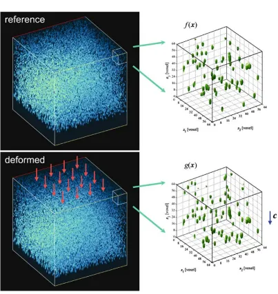
LSCM provides discretized volume images visualizing three-dimensional structural patterns of fluo-rescent markers in a transparent sample. In this study, the combination of digital volume correlation (DVC) and confocal images is used to achieve three-dimensional full-field deformation measurements as an extension of the vision-based surface deformation measurement techniques, well-known as dig-ital image correlation (DIC) [10]. The basic principle of the DVC is schematically illustrated in Fig. 2.5. Two confocal volume images of an agarose gel with randomly dispersed fluorescent particles are obtained before and after mechanical loading.

(41)

16

Digital Volume Correlation (DVC)

Principle of DVC

LSCM provides discretized volume images visualizing 3-D

structural patterns of fluorescent markers in a transparent

sample. In this study, the combination of digital volume

correlation (DVC) and confocal images is used to achieve 3-D

full-field deformation measurements as an extension of the

vision-based surface deformation measurement techniques,

well-known as digital image correlation (DIC). The basic

principle of the DVC is schematically illustrated in Fig.

2. Two confocal volume images of an agarose gel with

randomly dispersed fluorescent particles are obtained before

and after mechanical loading. Then, the two images are

subdivided into a set of subvolumes that are centered on the

points of interest. Using each pair of corresponding

subvolume images, the respective local displacement vector

can be obtained from 3-D volume correlation methods.

Consider two scalar signals

f

(

x

) and

g

(

x

) which

represent a pair of intensity patterns in a sub-volume

W

before and after a continuous mapping,

_b

y x

_{ð Þ}

:

x

_!

y

,

respectively. Assuming that the signal is locally invariant

during the mapping,

f

_{ð Þ ¼}

x

g

_ð

y x

_{ð Þ}

_Þ

, subvolume-wise

cor-relation matching can be obtained by finding an optimal

mapping that maximizes the cross-correlation functional

defined as

m

_{ð Þ ¼}

_b

y

Z

f

_{ð Þ}

x

g

_ð

y x

_{ð Þ}

_Þ

d

W

x

ð

1 Þ

The methodology is illustrated using a translational

vol-ume correlation, which is presented below. The continuous

mapping is assumed to be a rigid translation,

y

_¼

x

_þ

c

,

and the cross-correlation function is represented as a

function of a displacement vector

c

as

m

_{ð Þ ¼}

c

Z

f

_{ð Þ}

x

g

_ð

x

_þ

c

_Þ

d

W

x

ð

2 Þ

Fig. 2 Schematic illustration of the digital volume correlation (DVC)

Exp Mech

Figure 2.5: Schematic illustration of the principle of digital volume correlation (DVC)

m(ˆy) = Z

f(x)g(y(x)dΩx. (2.6)

The methodology is illustrated using a translational volume correlation, which is presented below. The continuous mapping is assumed to be a rigid body translation, y = x+c , and the cross-correlation function is represented as a function of a displacement vectorcas

m(c) = Z

[image:41.612.117.520.63.490.2]

(42)

The cross-correlation function can be written using Fourier transforms as

m(c) =F−1[F[f(x)]∗F[g(x)]], (2.8) where the Fourier transform off(x) is defined as

F[f(x)] = Z

f(x)e−ik·xdΩx, (2.9)

and * denotes the complex conjugate. The discrete cross-correlation function can be computed efficiently by using the fast Fourier transform (FFT) algorithm. Then, the rigid body translation vectorccan be estimated from the location of the cross-correlation peak with respect to the origin. Finding the displacement vector c from the discrete cross-correlation function is straightforward and provides half-voxel accuracy. Determining the displacement vectorcwithin subvoxel accuracy generally requires fitting and interpolation of the correlation function near the peak. Various fitting models have been used in the past [9, 48], employing somewhat arbitrary assumptions that the cross-correlation function near the peak can be approximated by a Gaussian or a parabolic function. The subvoxel accuracy of such peak-finding algorithms is determined by the choice of fitting function as well as the size of the fitting window. In this study, a three-dimensional quadratic polynomial fitting is used to fit the correlation function near the peak and hence provides improved subvoxel accuracy over previously used lower order fitting polynomials.

(43)

18 deformation fields is presented.

2.2.2 Stretch Correlation Algorithm

Assuming a general homogeneous deformation of each subvolume, the deformation field can be written as

ˆ

y(x) =Fx+c, (2.10)

with a deformation gradient tensorF=I+∇uand a displacement vectoru. Therefore, any uniform deformation in three-dimensions can be represented with a total of 12 parameters which consist of three displacement components and nine displacement gradient components. Optimal programming in three-dimensions for a total of 12 degrees of freedom (DOF) is computationally expensive in conventional correlation algorithms. Alternatively, the general homogeneous deformation can be represented using a polar decomposition of the deformation gradient tensor as

ˆ

y(x) =RUx+c, (2.11)

where R is the orthogonal rotation tensor and U is the symmetric right-stretch tensor. Then, the general homogeneous deformation in three dimensions is represented with six stretch, three rotation, and three translation components. Depending on the dominant mode of the deformation of interest, the correlation algorithm can be modified to include additional optimization parameters selectively. A digital volume correlation algorithm that includes three rotational degrees of freedom has been presented previously [46]. In this study, assuming small rotations and small shear stretch components, three normal stretch components are included as additional correlation parameters in the FFT-based DVC algorithm, as an extension of the stretch-correlation algorithm developed for large deformation measurements in two dimensions [22]. Neglecting the small rotations, the mapping of a pure homogeneous deformation and a rigid translation is written as

ˆ

(44)

When the loading axes are aligned with the global coordinate axes so that the shear stretch compo-nents are small, the invariant condition can be written as

f(x)≈g(Ux+c), (2.13)

where U denotes the diagonal part of U. Then, the six optimization parameters for the stretch correlation in DVC algorithm are{c1, c2, c3, U11, U22, U33} . In the case of a pure stretch problem without any translation, a simple coordinate transform into a logarithmic scale converts the stretch correlation problem into a simple translational correlation problem. However, when there is a non-zero translation, the coordinate transform cannot be directly performed in the spatial-domain to achieve the stretch correlation. Therefore, an equivalent invariant condition of Eq. (2.13) in the Fourier domain is considered to implement the stretch correlation in the Fourier domain as

||U||F(Uk) =eik·cG(k), (2.14) where, again, F(k) and G(k) represent Fourier transforms of f(x) and g(x), respectively. Then by using the Fourier power spectrums only and therefore dropping the phase term, a translation-invariant stretch-correlation problem can be achieved in the Fourier domain. A stretch cross-correlation function to be maximized for determining the three axial stretch components neglecting the determinant of the Jacobian is shown as

m(U) = Z

|F(Uk)||G(k)|dΩx. (2.15)

The stretch correlation problem in the Fourier domain can be transformed into a translational correlation problem in a log-frequency domain as

e

m(η) = Z

(45)

20

where ξ = logbk, η = logbU, and b is an arbitrarily chosen logarithmic base. The translational

correlation problem in the log-frequency domain can be easily solved using Eq. 2.8. Finally, the three axial stretch components can be obtained from the optimal vector η in the log-frequency domain as

U11=bη1_, _U22₌_bη2 _and _U33₌_bη3_. _(2.17)

Figure 2.6: Ilustration of the

stretch-correlation procedures using a

one-dimensional (1D) example The accuracy of the obtained stretch

compo-nents depends strongly on the spectral content of the original signals. If the signals are already band-limited, special considerations, such as normalizing the power spectrums and employing the Hanning window, must be included to achieve robust stretch correlations. Also, in the numerical implementa-tion of the stretch correlaimplementa-tion algorithm, incorpo-rating zero-padding of the signals before Fourier transforms can improve the overall accuracy of the stretch correlation algorithm by providing ideal in-terpolations of the Fourier transforms at a cost of increased computational load.

In Fig. 2.6, the stretch-correlation procedures are illustrated for a one-dimensional example. Two reference and deformed signals representing 10% of uniform strain are shown in Fig. 2.6 (a). The Fourier power spectra of the two signals are shown

(46)

in the log-frequency domain as shown in Fig. 2.6 (e), the translational correlation as presented in Eq. 2.16can be applied to find the one-dimensional stretch value. Extension of the one-dimensional stretch-correlation into two dimensions or three dimensions is straightforward as long as the rotations and shear stretches are small.

Figure 2.7: Two-dimensional

projec-tion of confocal subvolume images (a)

be-fore and (b) after uniaxial compression of

10% inx3-direction

In the implementation of three-dimensional stretch correlation, two-dimensional projections of the three-dimensional subvolume images were used to circumvent the geometrically increased computa-tional load after the zero-padding, as shown in Fig. 2.7. Essentially, the stretch correlations using the large zero-padding were conducted in a reduced di-mension for computational efficiency. Three sepa-rate two-dimensional projections were made so that three sets of two stretch components could be ob-tained. From the six stretch values, three stretch components (U11, U22, U33) were obtained by

com-puting the average of the two corresponding stretch components. Once the three axial stretch compo-nents are found, the translation vector ccan be de-termined more accurately by conducting the stretch-compensated translational correlation using

m(c) = Z

e

f(x0)g(x0+c)dΩx, (2.18)

(47)

22

the stretch part of the deformation is compensated, a more accurate translation vector c can be obtained. The stretch correlation and the translational correlation were conducted iteratively to achieve converged results. For all experiments executing the stretch and translational correlation twice yielded sufficient convergence based on a mean difference criterion, where the mean and stan-dard deviation of the difference of the before and after displacement matrices were compared (this is similar to the least-square error estimate). Such an iteration process is equivalent to the iterative optimization of a correlation coefficient in conventional image correlation scheme conducted in the two-dimensional spatial domain.

Finally, the displacement gradients were computed by using a three-dimensional least-square fitting of each displacement component in a 3 x 3 x 3 grid of neighboring data points. Although a more sophisticated smoothing or filtering algorithm can be employed before or during the gradient calculation to obtain smoother strain fields, no such algorithm was used in this study to assess the performance and robustness of the proposed DVC algorithm. Once the displacement gradient fields are determined, either infinitesimal or finite strain values can be computed from the displacement gradient fields.

2.3 Experimental Procedures

Agarose test specimens were prepared from a 1% weight-in-volume (w/v) solution of agarose (J.T. Baker, NJ) in standard 0.5X TBE buffer (Tris/Borate/EDTA, pH 8.0). The agarose solution was heated until molten, and carboxylate-modified red fluorescent (580/605) polystyrene microspheres (Invitrogen, CA) of 1 µm diameter were injected into the liquid agarose. The nominal volume fraction of fluorescent markers in the gel was 0.3%. The mixture was cast into a pre-chilled Teflon mold mounted onto a glass plate. Samples were left at room temperature for 5 minutes to solidify.

(48)

(Sigma-Aldrich, MO) of 100µm diameter were added to the mixture before casting. For spherical inclusion measurements describing a soft inclusion of a hard matrix, a burst of air was injected into the molten agarose gel to allow the formation of voids inside the material. The air inclusions (bubbles) were consequently imaged and a particular isolated bubble (only bubble within entire field of view) with a diameter of 200µm was chosen.

Figure 2.8: Loading fixture for

uniax-ial compression of soft materuniax-ials mounted

onto a laser scanning confocal microscope To apply uniaxial compressive loading to the

sample while imaging, a miniature loading-fixture was built and mounted directly on the microscope stage of an inverted optical microscope as shown in Fig. 2.8. The sample was kept immersed in the buffer solution to prevent swelling or shrink-ing durshrink-ing the test. The compressive loadshrink-ing was achieved by translating a micrometer head with a resolution of 1 µm. For all experiments the imposed strain increments were controlled by the micrometer (Mc Master-Carr, Los Angeles, CA) and were calculated using the dimension of the specimen and the imposed loading (displacement)

Quantitative characterization of 3D deformations of cell interactions with soft biomaterials