Abstract—The increase in mobile communications traffic has
led to heightened interest in the use of deterministic propagation methods together with digital building and terrain databases for propagation prediction in urban areas. Ray methods have been particularly popular, and there are many papers in the literature describing the performance of various approaches to ray tracing.
This paper will describe a powerful, recently developed, three-dimensional (3-D) software suite for urban propagation modeling which, although based on 3-D ray tracing (using images), draws upon an ensemble of propagation tools including physical optics using the fast far-field approximation, the parabolic equation ap-proximation for propagation over multiple buildings, and uniform theory of diffraction (UTD).
Many ray-tracing methods determine ray paths between the transmitter and a single arbitrary receiver. This paper adopts an approach of a transmitter to a multiple receiver technique, resulting in greatly reduced computational times.
The associated method can handle both indoor and outdoor propagation on both flat and undulating terrain. Terrain is repre-sented as a set of triangular two-dimensional (2-D) patches, while buildings and clutter are represented using layers of polygons.
I. INTRODUCTION
T
HIS PAPER describes a ray-based planning tool that uses the method of images approach. The method of images, combined with the uniform theory of diffraction (UTD), is a high-frequency approximate method which has been applied to urban UHF propagation by a number of authors [1]–[11].All of these methods calculate the images of a transmitter relative to one arbitrary receiver, up to some maximum order. In contrast, the method we use involves a strategy that generates images of a transmitter relative to multiple receivers.
Another possible method is the ray-launching method used by Liang and Bertoni [14] which we decided not to use, although we did employ their formulation for Fresnel zone calculations. In particular, we adopted this approach for horizontal propaga-tion while Liang and Bertoni [14] considered the same approach for over rooftop propagation.
In the method described in the next section, a significant re-duction in computational time is achieved by the following.
• Use of a sectorized approach to reduce the time spent for ray tracing and calculation of angular components of diffraction coefficients.
• Use of dynamic visibility lists similar to Coupe et al. [6] and Agelet [8].
Manuscript received November 30, 1998; revised April 15, 1999.
The authors are with the Department of Electrical Engineering, Trinity Col-lege, Dublin, Ireland (e-mail: [email protected]).
Publisher Item Identifier S 0018-9545(00)02555-X.
• The process of compiling visibility lists is combined with the process of calculating field strength on the receiver grid.
The formula for doubly diffracted rays is that used by Kanatos et al. [7] and is due to Rustako et al. [10].
Our method is different from all the others mentioned above in that it can include irregular terrain. The theoretical limit over which the terrain discretization varies can be as small as 2 m.
Many ray-tracing methods define a maximum order of reflec-tions and maximum order of diffracreflec-tions . The method is then said to find the solution of an problem. When solving elec-tromagnetic wave propagation-related ray-tracing methods, it is helpful to neglect rays which contribute very little to the overall computed field strength. This is part of the inevitable tradeoff between accuracy and computational complexity. In other cases because of the very nature of the geometry, some ray paths never occur.
The following categories for an ray trace are included.
• The unobstructed ray between the transmitter and an ob-servation point.
• We include all valid three-dimensional (3-D) geometrical optics paths excluding those involving two consecutive terrain reflections and those involving reflections from flat rooftops. The excluded occurrences are considered to be rather unlikely since the former would require reflection from the underside of an arch-shaped building while the latter would require a reflection over a rooftop to an obser-vation point above roof level. In practice, all obserobser-vation points are at street level.
• For UTD horizontal edge diffraction, we restrict the value of such that . In this case, the corresponding number of reflections is . As an alternative we may include multiple horizontal edge diffraction using the two-dimensional (2-D) parabolic equation method of Janaswamy [13]. It is also possible to substitute the fast far field (FAFFA) method [15] for the parabolic approach when calculating the propagation over rooftops.
• We include the case of vertical corner diffraction with the restriction of followed immediately by terrain reflection or further arbitrary wall reflection.
II. IMPLEMENTATION OF THERAY-TRACINGMODEL
The method of images is intrinsically recursive. A planar sur-face which is visible to the transmitter will give rise to a single first-order image. This image can be considered to be a virtual
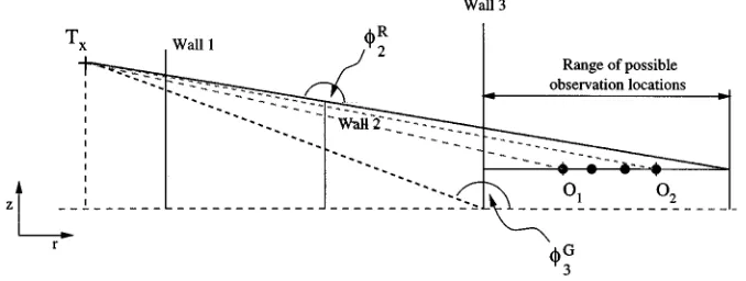
Fig. 1. Representation of method of images incorporating a sectorized approach containing groups of receivers.
Fig. 2. The unfolding of the ray path shown in Fig. 1 including reference angles and , which restrict the range of possibilities for an observation point.
source with respect to points in its zone of illumination as shown in Fig. 1.
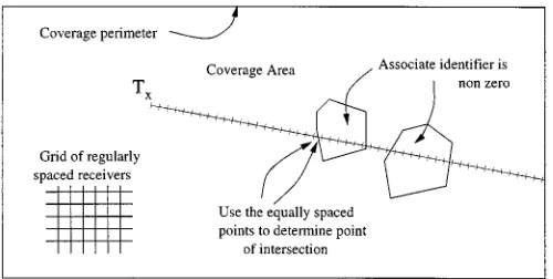
The coverage area is defined to be a uniform rectangular grid of receivers, and the coverage perimeter is defined to be the perimeter of this area.
A zone of illumination is associated with each source. For an image, this is the space on the opposite side of the plane con-taining the wall which generated the image. Representing the wall as a line segment in two dimensions results in an area of il-lumination (see Fig. 1) which is enclosed by the points
and , where and are the extremities of the line segment and and are the projected points on the perimeter of the area.
Along the line segment in the vertical plane (see Fig. 2) the zone of illumination is restricted by the maximum angle
made with the rooftop of a building or the angle made with the height of the observation on the perimeter when
.
For the transmitter the zone of illumination is only con-strained by the ground and the perimeter unless directional antennas are to be used.
First-order images can give rise to second-order images, second to third, and so forth.
A virtual source is characterized by:
1) position ( being the height);
2) generating surface or edge;
3) generating source (either the transmitter of a virtual source);
4) order and its nature (image or diffracting edge).
A. Data Structures
For the purpose of reference, a regular two-dimensional grid
of receivers is established over the coverage area. As a rule of thumb, the mesh size of this grid should be no greater than about 2 m for reliable performance. A number of layers are de-fined with reference to this grid.
Given that the th building in the coverage area is assigned an identifier , we then say that a building identifier layer is an array consisting of nonzero identifiers corresponding to a building location or terrain location in the region of interest. In the case of a terrain location we insert an entry with value to indicate that we are not dealing with a polygon or polyhedra structure. An observation points layer is an array of three-di-mensional points whose vertical projection falls on a grid point over which there is no building. The height of observation points is the terrain height plus a fixed height. Surface points form an array of 3-D points lying either on the terrain or on the roofs of buildings lying directly over grid points. Finally, there is a field
strength layer which is an array for accumulating the complex
valued field.
[image:2.612.127.466.284.412.2]The zone of illumination of each source is divided into sectors (see Figs. 1 and 2).
When constructing ray paths and checking their validity, the process can be decomposed into a horizontal and a vertical sweep.
The horizontal sweep checking the validity of an observation point such as (see Fig. 1) will involve tracing from that ob-servation point back to the transmitter to ensure that the wall reflections are valid. If any point on the sector is horizontally invalid, then all points in the sector will be invalid—so that only one point needs to be checked. This results in large computa-tional savings and is one of the main advantages of the sector-ized approach.
In the case of the vertical sweep, the ray path is unfolded to show the route that the path takes in the plane. In Fig. 2, we refer in particular to as the angle made with the positive axis, ground level point of the th wall, and the transmitter. Also, we refer to as the angle made with the positive axis, roof height for the th wall of the given sector and the transmitter. In particular, we require defined to be the maximum over the list of angles and defined to be the last angle in the list
of angles . The two angles and define the range
over which an observation point can result in a valid reflection for the given wall list. It should be noted that valid ray paths only exist when the line segment of say intersects with every wall along that path.
In the case of an image sector, we define these angles by con-sidering the first grid point in the sector, ray tracing back to the transmitter, recording as we go, the wall top and bottom edge elevation angles with respect to the image.
C. Visibility List Construction
Before delving into the visibility list construction, we must first say something about the points at which we wish to calcu-late field strengths. In our implementation, we begin our field computations at the transmitter. We are interested in computing the field at all observation points (transceivers in the case of mobile communications) in the coverage area. Since the cov-erage area is defined to be a rectangular grid, it follows that the perimeter is automatically discretized according to the grid step size of this grid. To compute the fields due to the transmitter, each transmitter sector is handled in turn starting with the first chosen point of reference on the perimeter along with its adja-cent point traveling anticlockwise (this is shown by and in Fig. 1).
Within each sector starting at the transmitter we begin at the grid point within the sector that is closest to the transmitter and move outwards. At each grid point, we calculate and as
is found by locating the type identifier from the closest sur-rounding grid points of the list of coverage receivers. If the identifier of a surface point has a value of 1 and the value at the next point is greater than 1, then we have passed an edge into a building. The intersection of the building polygon with the line segment gives the location of the building point intersect . A triple where is the identifier on th building and the identifier of the th wall is appended to a direct LOS (DLOS) list. This is similar to the radial sweep algorithm similar to that of Agelet et al.[8] except that the list is updated as we travel from one sector to the next sector in the zone of illumination. In the adjacent sector in the zone of
illumi-nation a new wall is found. If from the previous
sector, a new triple must be then added to the DLOS list, and we have encountered a diffraction point also.
The list of all partially obstructed line-of-sight (OLOS) walls encountered within a sector is contained in an OLOS list. This list along with an adjacent list is stored at any one time. If a new sector is traversed, then the old one is replaced with the adja-cent OLOS list, and the next OLOS has to be determined. Any candidate for inclusion is first checked against the short OLOS list and only if it is absent do we need to check the FLOS list. In this way we maintain, for each source, a set of four visibility lists, namely, the DLOS list, the current OLOS list, the previous OLOS, and the FLOS list.
In the case where no wall is encountered in a sector, a null item is added to the DLOS list.
On completion of the scanning of the grid, the DLOS list is examined to determine which vertical edges are also visible, and this information is stored in a visible vertical edge (VVE) list. We will return to this later when considering diffraction.
Having calculated the DLOS and OLOS lists, we can now calculate the first-order images. Starting with the first wall in the DLOS visibility list about the transmitter, we construct the first-order image of the transmitter in this wall and insert it into the image tree. We then find the transmitter image in the second wall and so on until we reach the end of the DLOS list. We then carry out exactly the same procedure using the OLOS list. The VVE list items are added to the tree also, but are labeled as being generated by diffraction rather than reflection as in the other case.
At each LOS observation point, we calculate and accumulate the field contribution from the source until we encounter the perimeter.
D. Terrain Reflections
points and calculate the image of the source in that plane. We examine all the grid points con-tained in the illumination zone of the terrain image. In the case of grid points which correspond to observation points, we ac-cumulate the contribution of this path to the field in the manner described below. In the case of grid points which are contained in buildings, we find the wall of the building that the ray inter-sects and compute the next order image in that wall (this image is not added to the image tree). We now compute a zone of il-lumination for this image noting that this depends on the zone of illumination of the terrain image. We accumulate field values for observation points contained within this zone of illumina-tion.
E. Diffraction
All diffracting edges are assumed to be either vertical or hor-izontal. The two cases are treated differently.
1) Horizontal Edge Case: We will first consider horizontal edge diffraction. The appropriate edges are found when traversing the sectors radially. Recall that as we move out along the sector, we calculate the surface elevation angle at each grid point . We also determine if we have just left an outer wall behind us. This is done by examining changes in the value of the building identifier grid. If we have just passed an outer wall and the value of at the previous grid point is greater than , then the top edge of that outer wall is visible.
Having identified a diffracting edge we now continue to move along the sector. At each observation point beyond the diffracting edge, we compute and accumulate the contribution to the field until we encounter another wall and perform the same operation again until we reach the perimeter. One special exception occurs when we find an observation point which is directly visible from the transmitter, but was found to be behind a building when performing the horizontal sweep. In this case, we must revert this back as a DLOS list contribution.
2) Vertical Edge Case: Vertical wall edges behave in a somewhat similar manner to image sources. One difference is that the zone of illumination does not include the wedge containing the edge, and it is further restricted to points with elevation angles lying between edge extremity elevation angles, where all elevation angles are taken with respect to the source illuminating the edge.
After we have traversed all the sectors (in the illuminated zone) of a source, we examine the DLOS list to find the vertical edges visible to the source. Recall that there will be a triple of entries in this list for each sector of the source. The triple will either be a null triple or a triple due to an intersection with a wall. Note also that sector entries appear in anticlockwise order. This means that when we step through the list we are ef-fectively scanning the zone of illumination.
[image:4.612.303.553.61.187.2]Referring to Fig. 3 we step through the DLOS list. We ex-amine the first entry and record the wall identifier, which may be null valued, as the “previous” value. We then proceed to the next entry and compare its wall identifier with the previous value. There are two possibilities. The first is that both identifiers are the same in which case the building identifier is stored as the new previous value, and we proceed to the next entry. The other
Fig. 3. The decimation of a profile used to locate over roof diffraction, DLOS, and OLOS in one traversal.
possibility is that the two identifiers differ, and this can occur in four different ways giving rise to four cases.
These are as follows.
1) Null followed by a wall—we deduce that the right-hand corner of that wall is visible.
2) Wall followed by a null—we deduce that the left-hand corner of the wall is visible.
3) Wall followed by contiguous (same building and touching) wall—we deduce that the edge where the two walls meet is visible.
4) Wall followed by a noncontiguous wall—for this case, we make use of the intersection points in the DLOS list cal-culating their distances from the source. We compare the current and previous distances and there are three cases of interest.
• The current distance is less that the previous dis-tance, and we deduce that the right-hand corner of the wall corresponding to the current identifier is visible.
• The current distance is greater than the previous distance, and we deduce that the left hand edge of the wall corresponding to the previous identifier is visible.
• In the case of equality, we include no edge. In this way, we work through the entire DLOS list for each source. When this task is complete, we are in possession of a list of visible vertical edges for that source. Each of these visible vertical edges behaves like an image as described above and is inserted into the source tree at one order higher (the lowest order is the transmitter) than that of its generating source.
III. POSTPROCESSING AND ADDITIONS TO
RAY-TRACINGMETHOD
A. Calculation of Field Strength
In the case of the transmitter, the field contribution depends only on the distance separating the transmitter and the observa-tion point.
tance back to the image point. The contribution at any other ob-servation point within the sector uses the same diffraction co-efficient and distance to the image point; the difference being the distance to the diffraction edge point from the observation point.
In the case of horizontal edge diffraction, the method is sim-ilar to that of vertical edge diffraction except that the angle made with the rooftop from the observation point is changing, and, hence, the diffraction coefficient has to be recalculated for each new observation point along a sector.
B. Fresnel Zone Criterion
In using geometrical optics to calculate the field strength con-tribution of a reflected image to the observation points lying along a sector, it is necessary to ensure that the first Fresnel zone is totally intercepted. Therefore, before proceeding outwards along a sector, we calculate the maximum allowable distance, from the image, of an observation point on the sector that can satisfy the Fresnel zone criterion with regard to the reflecting wall and source. The physical optics approximation, as given by Ishimaru [12], is used to calculate the field strength contribu-tion at observacontribu-tion points located at greater than this maximum Fresnel distance as we proceed outward along the sector. For the case of ray paths containing reflections, a maximum al-lowable distance must be calculated for each of the reflecting walls. The distance of an observation point from each wall must be compared with its maximum Fresnel length. The contribu-tion of a sequence of wall refleccontribu-tions to an observacontribu-tion point will typically consist therefore of a number of wall reflections, for which the geometrical optics formula is valid, and a number of wall contributions that require the physical optics approxima-tion.
As we proceed outwards along a sector, each observation point must in turn be examined to see if its Fresnel zone is suf-ficiently unobstructed for the image source contribution to be valid. The procedure for this is as follows. At the first observa-tion point as we proceed outward we examine all grid points on a line orthogonal to the radial sector up to a given distance on either side of the first observation point, where is the width of the Fresnel zone of the most distant observation point. If an ob-struction is encountered in the orthogonal scanning, then a new maximum observation point distance is calculated in ac-cordance with this. Since the Fresnel zone width is now smaller due to the fact that , it follows that the must be replaced with a new maximum Fresnel distance . This new distance will be shorter in accordance with the change between and . This procedure is repeated for subsequent
observa-the transmitter, can be calculated using observa-the parabolic equation method. To employ in particular the two-dimensional method of Janaswamy [13] in a 3-D model, we use it to calculate the path-loss along the radial lines of each radial sector. This in-volves constructing a 2-D profile of height versus radial distance of surface points lying along the radial line. After calculating the path-loss along the profile, interpolation is then used together with previous radial path-loss to calculate the contribution at each observation point that lies within the sector.
D. Optimization of Ray Tracing
For a dense grid of receivers it is useful to minimize the number of times the diffraction coefficient must be calculated and also the amount of time spent on validating ray paths.
In this model, this has been accomplished by taking advan-tage of the fact that the ray-tracing process can be decomposed into a horizontal two-dimensional component and a vertical two-dimensional component. Referring to Fig. 1 it is clear that if the ray path terminated by is horizontally valid, then so also is the ray path to . It only remains to verify that lies within the vertical plane of illumination as illustrated in Fig. 2. A potential computationally expensive pitfall of ray tracing is the requirement to find a list of all buildings intersecting a given line and to order them in terms of increasing distance along the line. We have avoided this pitfall through the use of a building identifier layer. Agelet et al. [8] use a quadtree to provide lo-calized building data in their approach. Our approach involves traversing the line segment in units of the grid step size and at each point on the line segment checking the local value of the building identifier layer. Thus, a list of buildings, ordered ac-cordingly as they intersect the line segment, is built up. This ap-proach is more efficient than a method which involves finding all buildings in the locality that intersect the line segment and then requiring the use of a sort routine to order them.
IV. RESULTS
A. Example 1: 2-D Ray Tracing Versus Combined Field Integral Equation Technique
Fig. 4. Two building microcell used to calculate path-loss profile.
Fig. 5. Comparison of path loss for 2-D ray tracing and CFIE at 300 MHz along indicated line in Fig. 4.
The ray tracing shows good agreement with the CFIE for rel-atively simple microcells.
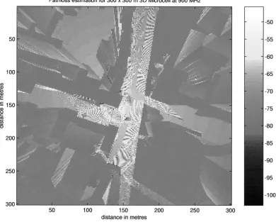
B. Example 2: 3-D Ray-Tracing Prediction
An illustration of path-loss predictions for the full 3-D case is shown in Fig. 6. The path-loss extends over the range 20–120 dB, with the colors varying from yellow (20–60 dB) to orange (60–100 dB) to red (100–120 dB). The antenna was positioned
above roof level at the position of to allow
for transmission over the surrounding buildings. The buildings themselves are colored white.
The maximum allowable number of ray path interactions in this prediction was four and the maximum allowed number of vertical edge diffractions was one. The computation time for this calculation was approximately 32 min and the prediction was carried out on a 300 300-m region with step size of 1 m. The total number of building facets was 879. The prediction was carried out for the city of Metz in France. The computer used was a 200-MHz RS6000 with Power 2 architecture. The computational time is not broken down into wall list search
times and ray-tracing times since the process of determining the wall visibilities is intertwined with the calculation of the ray trace.
C. Example 3: Ray-Tracing Prediction Versus Measurements
A measurement campaign of the Upper Mount Street area of Dublin resulted in the measurement of 3153 distinct path-loss values calculated along specific trails. The loss was measured with respect to a fixed antenna emitting at 481.5 MHz located at 5 m above street level.
A ray trace with four reflections and one diffraction was used to calculate the path loss over the same region. A comparison with the measurement results is shown in Fig. 7. The results were shown to give very good agreement. The shift in values is due to the fact that the path loss is normalized. The ray trace was produced for approximately 426 buildings on a 600 500 grid with a computational time of 514 s on a Pentium Precision 610 PC (550 MHz).
V. CONCLUSION
In essence, ray tracing is concerned with finding most or all of the propagation paths that connect a transmitter with a given receiver. Thus, it is usually formulated on a point-to-point basis. When we wish to calculate the field strength at each point of a grid of receivers, the point-to-point approach has a number of disadvantages.
1) It leads to unnecessary repetition since the calculations for one grid point must be essentially repeated for all other grid points. Thus, the total computation time is propor-tional to the total number of grid points, and this can be expensive for a dense grid over a large area.
2) Effort must be expended in determining which ray paths are significant enough to be included. Thus, in [2] Fresnel zones are among the methods introduced to limit the number of obstacles in the environment that need to be examined for interactions in a transmitter—a single receiver system.
In the approach we have adopted these drawbacks are over-come by using an algorithm based on a point-to-area calculation. This allows us to introduce time-saving approximations for ad-jacent receivers or take advantage of the fact that certain calcu-lations need only be done once for points on radial lines.
In [2], precalculation of visibility lists is used to speed up the calculation. In 3-D models this is an inefficient approach as over building propagation makes it very difficult to predict visibility of facets. A dynamic calculation of visibility lists as described below is more suitable for the 3-D case. The approach is similar to that described in Lambert and Coupe [6], where the visibility algorithm allows deductions to be made about the visibility of corners of buildings.
Fig. 6. Path-loss prediction for 3-D outdoor ray tracing at 900-MHz propagation. The observation point grid size is 3002 300 on an area of 300 2 300 m.
[image:7.612.55.546.427.727.2]APPENDIX
A. Details of Implementation
The software for this model is written in C++ using object-oriented programming (OOP). The Library of Efficient Data types (LEDA) is used. The urban environment is represented by the City class. This consists of the following principle data members.
1) A base transmitter station as represented by a 3-D vector. 2) The South-West and North-East coordinates and step
sizes of the grid.
3) A 2-D complex array which is used to store the field strength values as they are accumulated at each re-ceiver grid point
4) A LEDA list of instances of the Building class. Each building is identified by its number on the list.
5) A 2-D integer array Building Number which is as-signed the identification number of the building within which the grid point lies or otherwise is just
as-signed .
6) A 2-D integer array Terrain Height which stores the terrain height multiplied by ten and converted to an integer value for the grid point .
The building class consists of a LEDA list of instances [17] of the wall class and a LEDA polygon. Each wall can be assigned its own reflection coefficient, if desired. In order to model ter-rain reflection, a Triangle class has been defined. Thus, to find the image of a transmitter at a terrain grid point , an in-stance of the triangle class is constructed using the two
neigh-boring terrain grid points .
The general algorithm for use of the software is as follows.
• The user selects the area to be modeled from a GUI or file plus the directional antenna to be used and the grid step and the mobile receiver height.
• The user can select whether the model to be run is: a) 2-D;
b) 2-D with Fresnel zone checking/physical optics; c) 3-D;
d) 3-D with Fresnel zone checking/physical optics; e) 3-D with Janaswamy parabolic equation method; f) 3-D with Fresnel zone checking/physical optics and Janaswamy method;
• The building data is read from an IGN contour database text file and the terrain elevation from an IGN dtm text file. IGN is a French geographical information database format for building and terrain data.
• The first set of images (for the real transmitter) is found. • The zone of illumination is calculated and visibility
lists drawn up for each image simultaneously as the field strength contribution at each observation point is calculated.
• The set of new images is found using the previous im-ages and their visibility lists and the previous procedure repeated.
• The sequence is terminated when the maximum number of ray path interactions is attained and the path-loss is then calculated for all observation points.
B. Indoor Version of Software
The algorithmic ideas are applied in the same way to indoor propagation as outdoor propagation, except that we have extra information due to doors, floors, and windows. Also, we can allow penetration of rays into and out of buildings taking into account specific penetration and reflection coefficients as part of the field strength calculation.
C. Surface Roughness
When taking into account roughness on a wall, we usually model this by using a corrugated surface in place of a straight face. This is quite difficult to model since we have many pe-riodic edges along one wall facet. Ray-tracing algorithms will not properly cope with this sort of arrangement, and these sort of factors should be left to integral equation-type methods.
ACKNOWLEDGMENT
The authors would like to acknowledge the European Union ACTS project entitled Software Tool for the Optimization of Radio Mobile System (STORMS) for their help in making this work possible.
REFERENCES
[1] K. H. Craig, “Impact of numerical methods on propagation modeling,” in Modern Radio Science 1996. Oxford, U.K.: Oxford Univ. Press, 1996.
[2] F. Ikegami, T. Takeuchi, and S. Yoshida, “Theoretical prediction of mean field strength for urban mobile radio,” IEEE Trans. Antennas Propagat., vol. 39, no. 3, pp. 299–302, 1991.
[3] H. R. Anderson, “A ray tracing propagation model for digital broadcast systems in urban areas,” IEEE Trans. Broadcasting, vol. 39, no. 3, pp. 309–317, 1997.
[4] M. C. Lawton and J. P. McGeehan, “The application of a deterministic ray launching algorithm for the prediction of radio channel characteris-tics in small-cell environments,” IEEE Trans. Veh. Technol., vol. 43, no. 4, pp. 955–962, 1997.
[5] K. Rizk, J.-F. Wagen, and F. Gardiol, “Two-dimensional ray tracing modeling for propagation prediction in microcellular environments,”
IEEE Trans. Veh. Technol., vol. 46, pp. 508–518, May 1998.
[6] J. M. Lambert, J. F. Sante, and J. M. Coupe, Geometrical Optimization
of the Raytracing Propagation Model.
[7] A. G. Kanatos, I. D. Kountouris, G. B. Kostaras, and P. Constantinou, “A UTD propagation model in urban microcellular environments,” IEEE
Trans. Veh. Technol., vol. 46, no. 1, pp. 185–193, 1997.
[8] F. A. Agelet, F. P. Fontan, and A. Formella, “Fast ray tracing for micro-cellular and indoor environments,” IEEE Trans. Magn., vol. 33, no. 2, pp. 1484–1487, 1997.
[9] G. Wolfle, B. E. Gshwendtner, and F. M. Landstorfer, “Intelligent ray-tracing—A new approach,” in VTSC, 1997.
[10] A. J. Rustako, N. Amitay, G. J. Owens, and R. S. Roman, “Radio prop-agation at microwave frequencies for line-of-sight microcellular mobile and personal communications,” IEEE Trans. Veh. Technol., vol. 40, pp. 203–210, Feb. 1991.
[11] M. F. Catedra, J. Perez, F. S. de Adana, and O. Gutierrez, “Efficient ray-tracing techniques for three-dimensional analyses of propagation in mobile communications: Application to picocell and microcell sce-narios,” IEEE Antennas Propagat. Mag., vol. 40, no. 2, pp. 15–27, 1998. [12] A. Ishimaru, Electromagnetic Wave Propagation, Radiation and
Scat-tering. Englewood Cliffs, NJ: Prentice-Hall, 1991.
[13] Janaswamy and B. Andersen, “Pathloss prediction in urban areas with irregular terrain topography,” COST 259, TD(98)060.
[14] G. Liang and H. Bertoni, “A new approach to 3-D ray tracing for prop-agation prediction in cities,” IEEE Trans. Antennas Propagat., vol. 46, no. 6, pp. 853–863, 1998.
Since 1996, he has been with the Department of Electronic and Electrical Engineering, Trinity Col-lege, researching the development and application of computational methods in electromagnetics. His current research interests include the propagation of UHF waves in urban environments and the use of adaptive antenna arrays.
Eamonn M. Kenny received the B.A. degree in mathematics and the M.Sc. degree in numerical analysis from Trinity College, Dublin, Ireland, in 1992 and 1994, respectively.
From 1995 to 1998, he was involved in the European Union project Software Tools for the Optimization of Radio Mobile Systems (STORMS). In particular, he helped develop and implement a large number of new electromagnetic wave equation techniques in urban and open environments. He is currently with Teltec Ireland, a telecommunication campus company at Trinity College, where he is involved in propagation model development for planning tools for radio mobile networks. In conjunction with this, he researches new techniques which utilize both ray tracing and integral equations in urban environments.