Elastic stability of columns with variable flexural rigidity under arbitrary axial load using the finite difference method

(1)

23 Numerical Methods in Civil Engineering

Elastic stability of columns with variable flexural rigidity under

arbitrary axial load using the finite difference method

M. Soltani

*

_{, A. Sistani}

**

ARTICLE INFO Article history: Received: September 2016. Revised: December 2016 Accepted: March 2017.

Keywords:

Elastic stability analysis Buckling load

Non-prismatic columns Finite difference method

Abstract:

In this paper, the finite difference method (FDM) is applied to investigate the stability analysis and buckling load of columns with variable flexural rigidity, different boundary conditions and subjected to variable axial loads. Between various mathematical techniques adopted to solve the equilibrium equation, the finite difference method, especially in its explicit formulation, requires a minimum of computing stages. This numerical method is therefore one of the most suitable and fast approaches for engineering applications where the exact solution is very difficult to obtain. The main idea of this method is to replace all the derivatives presented in the governing equilibrium equation and boundary condition equations with the corresponding forward, central and backward second order finite difference expressions. The critical buckling loads are finally determined by solving the eigenvalue problem of the obtained algebraic system resulting from FDM expansions. In order to illustrate the correctness and performance of FDM, several numerical examples are presented. The results are compared with finite element results using Ansys software and other available numerical and analytical solutions. The competency and efficiency of the method is then declared.

D

1. Introduction

Stability analysis of structural members such as beams and columns is a criteria factor in the design of different constructions. Therefore, the accurate calculation of the critical buckling loads and buckling modes of elastic members could help engineers to produce structures with satisfactory stability. There are a large number of researches devoted to the linear stability analysis of columns with constant cross-section. For non-prismatic beams subjected to axial forces, the stability analysis becomes more complicated due to the presence of variable coefficients in the governing fourth order differential equation. Regarding this, there are not any general closed-form solutions for exact estimation of buckling loads of non-prismatic beams; hence application of different numerical techniques have been carried out by researchers.

* Corresponding Author: Assistant Professor, Department of civil engineering, University of Kashan, Kashan, Iran ([email protected])

**MSc in Structural Engineering, K.N.Toosi university of Technology, Tehran, Iran ([email protected])

Elastic members whose cross-sectional profile changes smoothly through their longitudinal direction, known as non-prismatic members, are widely spread in a variety of engineering applications due to their conspicuous characteristics such as satisfaction aesthetic necessities and optimal distribution of weight.

The first investigation in this field was presented by Euler. He calculated the critical buckling load of columns under their own weight. Dinnik, Karman and Biot offered closed-form solutions for the equilibrium differential equations [1, 2]. On the other hand, Timoshenko derived the governing equilibrium equations and their closed-form solutions for various types of flexural members under different circumstances [3]. The exact solution for special types of tapered columns was proposed by Gere and Carter for the first time [4]. Frisch-Fay achieved critical buckling loads of prismatic elements by using analytical solution. The elements were surveyed with various boundary conditions and subjected to uniform axial force. He acquired the critical buckling load for a uniform strut that was excluded from sway at top and bottom by introducing two Bessel integrals and one multiple Bessel integral [5].

Ermopulos estimated the critical loads and the

(2)

Numerical Methods in Civil Engineering, Vol. 1, No. 4, June. 2017

corresponding equivalent buckling lengths of frame with non-uniform members based on slope deflection method [6]. FDM was applied by Iromenger to determine critical buckling load of tapered and stepped columns [7] whereas Smith adopted the energy method and symbolic analysis for evaluating buckling loads of the tapered columns [8]. Arbabi and Li presented a semi analytical approach for measuring buckling load of columns with step-varying profiles [9]. While Siginer studied the problem of buckling of tapered columns with linear variation of flexural rigidity [10], Sampaio and Hundhausen presented a mathematical model and analytical solution for buckling of inclined beam-columns. Overall, only one type of boundary condition (pinned-ends) was analyzed based on their methods and its exact solution was shown [11]. Wang et al.

illustrated closed-form solutions for stability analysis of columns, beams, arches, rings, plates and shells [12]. Li et al. investigated the stability analysis of bars with non-constant cross-sections. They calculated the eigenvalue of multi-step bars subjected to simple and complicated loads using Bessel’s functions [13, 14, 15]. Rahai and Kazemi formulated a new approach for the linear stability problem of tapered column members. The exact buckling load was calculated by combination of modified vibrational mode shape (MVM) and energy method [16]. Coşkun and Atay used variational iteration method to determine the critical buckling load of elastic columns with variable cross-sections [17]. Huang and Luo proposed a new and simple procedure to compute the critical buckling loads of beams with various boundary conditions subjected to arbitrarily axial in-homogeneity [18]. Okay et al. derived buckling loads and mode shapes of a heavy column by applying the variational iteration method [19]. Atay and Coşkun analyzed elastic stability of Euler columns with continuous restraint using variational iteration method (VIM) [20]. Atay applied a new approach, known as Homotopy perturbation method, to solve the buckling problem of non-prismatic columns [21]. Pinarbasi computed lateral-torsional buckling load of non-uniform rectangular beams by using homotopy perturbation method (HPM) [22]. Some researches applied the power series method to investigate stability behavior of different types of columns. In this method, displacements and other variable parameters such as flexural rigidity, axial load are approximated by polynomial functions. In order to achieve the exact result, the polynomial order must be increased. Eisenberger used this method to study stability and free vibration behaviors of a beam resting on variable two-parameter elastic foundations [23, 24]. Al- Sadder used this approach to solve the fourth-order ordinary differential stability equation of a non-prismatic beam-columns under uniform tensile or compressive axial force [25]. This method was then adopted by Asgarian et al. to investigate the lateral instability of tapered thin-walled beams with arbitrary cross-sections [26].

The abovementioned researchers investigated the problem of buckling only for special types of columns. Tapered and stepped columns and members with linear, quadratic and cubic variation of flexural rigidity were the most common forms of columns studied by many researches. The main purpose of this paper is calculating

the critical buckling loads for any type of columns with variable cross-sections such as: linear, polynomial and exponential variation of flexural rigidity under variable axial load based on the finite difference method with second order accuracy. In the first stage, fourth-order governing stability differential equation of a non-prismatic column under variable axial load is formulated and the related boundary conditions are then expressed. In the second stage, the equilibrium equation and boundary conditions are discretized by relating forward, central and backward finite difference formulations. In this regard, the expressions of derivatives of displacement represented in

the stability equation are presented based on

aforementioned numerical method. Finally, the system of finite difference equations culminates in a set of simultaneous and linear equations and the elastic critical buckling loads are calculated by solving an eigenvalue problem of the obtained algebraic system.

In order to demonstrate the accuracy and efficiency of this method to determine critical buckling loads of various types of non-prismatic columns, several numerical examples are carried out. Different representative load cases and various boundary conditions are considered. The obtained results are compared to finite element simulations using Ansys software and to other available numerical and analytical benchmarks. The stability analysis of uniform members as well as non-uniform ones can be done through the present method. Comments and conclusions are close to last section of the present paper.

2. Formulation of Equilibrium Equations

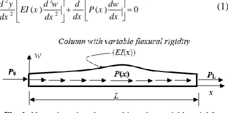
A non-prismatic beam with the length of L as depicted in Fig.1 is taken into account. In this study, Euler-Bernoulli beam theory for stability analysis of beam with variable cross-sections is adopted. Regarding this theory, the effect of flexural deformation is taken into account while the influences of shear deformation and rotatory inertia are negligible. The differential equilibrium equation for non-uniform column subjected to variable axial load can be expressed as follows:

2 2

2 ( ) 2 ( ) 0

d y d w d dw

EI x P x

dx dx

 _  _

  _ _

 

(1)

Fig. 1: Non-prismatic column subjected to variable axial force

Extending the above equation can be obtained as:

4 3 2 2

( ) ( )

( ). 2 ( ) .

( ) 0

d w dEI x d w d EI x d w

EI x P x

dx

dx dx dx dx

dP x dw dx dx

 

    

 

  

(2)

In the last formulation, E and w expressYoung's modulus of elasticity and vertical displacement, respectively. I and

(3)

25

P denote respectively the second moment of area and static axial load which can be both arbitrary over the beam’s length (x-axis).

Considering Fig. 2, two degrees of freedom exist at each node of elements in plane bending; vertical displacement in y direction ( ₁, ₂) and rotation about z-axis ( ₁, ₂). Therefore, for each end of a column depending on its condition, two boundary conditions can be considered as:

Pinned support:

w



0

and

2

2 0

d w

dx 

(3)

Clamped support:

w



0

and dw 0

dx  (4)

Free end:

2

2 0

d w

dx  and

3

3 0

d w P dw

EI dx

dx   

(5)

Fig. 2: Degrees of freedom for a column element

3. FDM Formulation of the Problem

The finite difference method is supposed to be a dominant numerical technique to solve differential equations with generalized end conditions. The Finite difference approach is a numerical iterative procedure that involves the use of successive approximation to obtain solutions of differential equations especially with variable coefficients. This numerical method is based on replacing each term of derivatives presented in the differential equation and its related boundary conditions with the finite difference formulations. The basis of this method is to approximate the function of derivatives with Taylor series expansions.

In order to apply the finite difference method to the equilibrium equation (1), the column member with length of L is assumed to be sub-divided into n parts, each of which equals to the length h L n/ , as shown in Fig. 3. Therefore, there are n+1 nodes along the column’s length, whose numbering starts with 0 at the left end finishes at n on the other side.

Fig. 3: equally spaced grid point along the column’s length in the finite difference method

According to the central finite difference method and in the presence of first to fourth order derivatives of vertical displacement of the considered element (2), derivatives of displacement for a discrete member are formulated as:

2

i h i h

w w

dw

dx h

  

 (7)

2

2 2

2

i h i i h

w w w

d w

dx h

   

 (8)

3

2 2

3 3

2 2

2

i h i h i h i h

w w w w

d w

dx h

      

 (9)

4

2 2

4 4

4 6 4

i h i h i i h i h

w w w w w

d w

dx h

       

 (10)

In which:

w

_i_₂_hare

w

_i_₂_hand

w

_{i h}_ ،

w

i ،

w

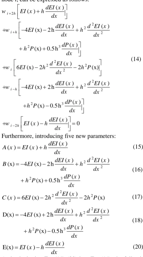
i h ،

vertical displacement of considered member in five points, located at equal distances from h.By substituting relations (7) to (10) in equation (2), and simplification, the governing differential equation in finite difference form at node i, can be expressed as follows:

2

2 2

2

2 3

2

2 2

2

2 2

2

2 3

( ) ( )

4 (x) 2 h

( )

(x) 0.5 h

( )

6 (x) 2 2 (x)

( ) ( )

4 (x) 2 h

(x) 0.5 h

i h

i h

i

i h

dEI x

w EI x h

dx

dEI x d EI x

w EI h

dx dx

dP x h P

dx

d EI x

w EI h h P

dx

dEI x d EI x

w EI h

dx dx

h P





 _ 

 

 



 _  





 



 

 _   _

 



 _  



 

2

( )

( ) 0

i h

dP x dx

dEI x

w EI x h

dx



 

 

 _  _

 

(14)

Furthermore, introducing five new parameters: ( )

( ) ( ) dEI x

A x EI x h

dx

  (15)

2 2

2

2 3

( ) ( )

(x) 4 (x) 2 h

( )

(x) 0.5h

dEI x d EI x

B EI h

dx dx

dP x h P

dx

   

 

(16)

2

2 2

2 ( )

( ) 6 (x) 2 d EI x 2 (x)

C x EI h h P

dx

   (17)

2 2

2

2 3

( ) ( )

D(x) 4 (x) 2 h

( )

(x) 0.5h

dEI x d EI x

EI h

dx dx

dP x h P

dx

   

 

(18)

( ) E(x) EI x( ) hdEI x

dx

  (20)

And substituting Eq. (15)-(20) into Eq. (14), the following expression is found:

(4)





















2

( ) B( ) ( )

( ) ( ) 0

i h i h i

i h i h

w A x ih w x ih w C x ih

w D x ih w E x ih

 

 

    

     (21)

Equation (21) should be written for n-1 grid points of a divided element; thus, n-1 equations are derived including n-1 unknown parameters (w₁,w w₀, ₁,....,w_n,w_n₁). In

order to solve the system of equation obtained based on the finite difference method, four extra equations eventuated from boundary conditions of the column are required. According to forward and backward finite difference formulations with second order accuracy, the introduced boundary conditions in Eqs. (3) to (5) can be respectively modified for the first and final points of divisions (i=0 and i=n) as follows:

Pinned support:

0

0 1 2 3

1 1 3

0 0

2 5 4 0

0

2 5 4 0

n

n n n n

w i

w w w w

w i n

w w _ w _ w _

     _ _ _ _       _ _ _ _  (22) Clamped support: 0

0 1 2

1 2

0 0

3 4 0

0

3 4 0

n

n n n

w i

w w w

w i n

w w _ w _

    _ _ _ _       _ _ _  (23) Free end:

0 1 2 3

2 2

0 1

2

2 3 4

1 1 3

2 2

1

2 5 4 0

( 0) ( 0)

0 ( 2.5 1.5 ) (9 2 )

( 0) ( 0)

( 0)

( 12 0.5 ) 7 1.5 0

( 0)

2 5 4 0

( ) ( )

(2.5 1.5 ) (9 2 )

( ) ( )

(12 0

n n n n

n n

w w w w

P x P x

i h w h w

EI x EI x

P x

h w w w

EI x

w w w w

P x L P x L

i n h w h w

EI x L EI x L

      _ _ _ _         _   _                           2

2 3 4

( )

.5 ) 7 1.5 0

( ) n n n

P x L

h w w w

EI x L   

       _     _  (24)

Therefore, finite difference approach in the presence of n equal segments along column member, constitutes a system of simultaneous equations consisting n+3 linear equations.

In the following, the simplified equilibrium equation through FD formulation is written for each grid point

without considering the corresponding equations of boundary conditions:

3 2

1 0 1

1 1

1 : ( ) B( )

1 1 1

( ) ( ) ( ) 0

L L

i w A x w x

n n

L L L

w C x w D x w E x

n n  n

                                              4 3

2 1 0

2 2

2 : ( ) B( )

2 2 2

( ) ( ) ( ) 0

L L

i w A x w x

n n

L L L

w C x w D x w E x

n n n

                                              5 4 3 2 1 1 1 3 3

3 : ( ) B( )

3 3

( ) ( )

3

( ) 0

. . .

1 1

1 : ( ) B( )

1 ( ) n n n L L

i w A x w x

n n

L L

w C x w D x

n n

L w E x

n

n L n L

i n w A x w x

n n

n L

w C x n                                                                          2 3 1 ( ) 1

( ) 0

n

n L

w D x n

n L

w E x n                              (25)

The final equation is obtained in a matrix notation as follows:

 

A _n_{  }₃_n ₃

 

w _n_{ }_{3 1}

 

0 _n_{ }_{3 1} (26) Where the expansion of coefficient matrix

 

A and

displacement vector

 

w

are:

 

1 0 1 2 1 1 . . . n n n w w w w w w w w                                      

(27a)

(5)

27  

0 0 0 . . . . 0 0

( ) ( ) ( ) ( ) ( ) 0 0 0 0 . . . 0 0

0 (x 2 ) (x 2 ) (x 2 ) (x 2 ) (x 2 ) 0 0 0 . . . 0 0 0 0 (x 3 ) (x 3 ) (x 3 ) (x 3 ) (x 3 ) 0 0 0 . . 0 0

0 0 0 . . . 0 0 . . 0 0

0 0 0 0 . . . 0 . . 0 0

0 0 0 0 . . . 0 0

0

a b c d e

f g h i j

E x h D x h C x h B x h A x h

E h D h C h B h A h

A

    



0 0 0 . . . 0 0

0 0 0 0 . . . 0 0

0 0 0 0 . . . 0 ( ( 2) ) ( ( 2) ) ( ( 2) ) ( ( 2) ) ( ( 2) ) 0 0 0 0 0 . . . 0 0 ( ( 1) ) ( ( 1) ) ( ( 1) ) ( ( 1) ) ( ( 1) )

0 0 0 . . . 0 0 0

E x n h D x n h C x n h B x n h A x n h

a b c d e

f g h i j

         

    

     



     

 

 _

(27b)

In which a a b b c, , , , , ... , , , ,....  i j j are obtained based on boundary conditions. The determinant of the coefficient matrix (A) must be zero to have non-zero answer. The smallest positive real root of the equation is considered as critical buckling load. It is worthy to note that the critical buckling load will be close to the exact value by increasing the number of segments.

In the following, the finite difference method is applied to study the stability analysis of columns with different conditions, such as variable flexural rigidity, various supports and variable axial load. The critical buckling load is calculated by using eigenvalue and the calculation procedure is done with the aid of MATLAB software [29].

4. Applications

The purpose of this section is to study the performance of finite difference method in buckling analysis of columns with variable flexural rigidity subjected to variable axial load. In this regard, several numerical examples are represented. The obtained results are then compared to other analytical and numerical solutions presented in literature and to finite element method by means of ANSYS code [30].

4-1 Example 1

In this example, in order to check the accuracy and exactness of the proposed FDM, five cases consisting the buckling analysis of cantilever and simply supported beams with constant or variable cross-sections are presented. In Case a, we investigated the critical buckling load of a stepped simply supported column subjected to compression load

P

. This column is composed of three parts, with uniform section at each segment, while the central part has a double moment of inertia. Young's modulus of elasticity

E=210(GPa), and the moment of inertia of the side part is

I0=2.1644e-9 m4. In case b, the critical buckling load is

carried out for a fixed-hinged non-prismatic column with rectangular cross-section whose depth is reduced to half at the pinned end with a

parabolic variation, while its width remains constant. Therefore, moment of inertia I

 

x can be expressed as:

 



2



5 .

0

1 x

I

x

I



A



(28)

Case c deals with the value of buckling load of a pinned end prismatic column under axial distributed load of

)) / ( 2 1 ( )

(x N0 x L

N   where N0=1 is the value at the

point

x



0

and

x



L

. Case d refers to the estimation of the linear buckling load of cantilever web-tapered beam with doubly symmetric I-section. In this case, the web height is made to vary linearly along the length so that, at the free end of the cantilever, the height is reduced. The material and geometrical properties are shown in the Fig. 4. All the considered columns and their corresponding cross-sections, boundary conditions, material and geometric properties are depicted in Fig. 4.

The calculated critical buckling loads for both first cases (a & b) are checked with the results obtained by finite element method using Ansys software [30]. Both mentioned members have been modeled using BEAM54 in ANSYS software. This member is a 1D beam element with tension, compression, and bending capabilities. The element has three degrees of freedom at each node: translations in the nodal x and y directions and rotation about the nodal z-axis. The obtained result of stability analysis of case c is compared with the buckling load evaluated by matrices solution proposed by Girgin and Girgin [27] whereas, in the case of tapered column, the linear buckling load acquired by present method is verified with results obtained by numerical method proposed by Soltani et al. [28]. The relative errors (



(%)

) between the results of present study and the abovementioned methods are also calculated.

(6)

Numerical Methods in Civil Engineering, Vol. 1, No. 4, June. 2017 Fig. 4: Prismatic and non-prismatic columns with different

boundary conditions: geometry, loading and material data.

Fig. 5: Columns with constant or variable cross-sections: variation of the relative errors (



) versus the number of

segments (n) along the column’s length.

A graphic illustration of the variation of the relative errors with the number of segments (n) considered in FDM is provided in Fig. 5. The following outcomes can be expressed after noticing the results represented in Fig. 5:

1. An outstanding compatibility between the elastic buckling loads acquired by current study and those computed from the other benchmark solutions is pinnacle.

2. Even by applying 30 segments in the beam’s length according to the suggested finite difference

method, the elastic buckling loads can be exactly reckoned bellow the acceptable error rate (1%). 3. When the number of segments in the applied

numerical method is increased to more than 50 pieces, relative errors (



) declined continuously to under 0.1%.

4. It is not indispensable to use more than 40 segments in finite difference approach, in order to obtain an acceptable accuracy on critical elastic buckling loads.

4-2 Example 2

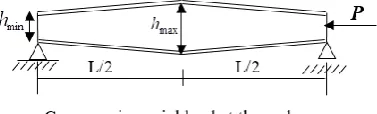
In this example, the linear buckling behavior of two sets of non-prismatic columns with pinned ends is investigated. The web height varies linearly from bigger section (hmax) at

the mid-span to the smaller one (hmin) at the pinned ends

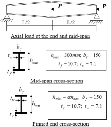
with different slopes, as shown in Fig. 11, while the geometrical parameters of mid-span section are remained constant. In both cases of uniform and non-uniform members, both flanges are uniform along axial axis and the considered columns are subjected to concentrated compressive axial load at two different positions of the column’s length, namely at the right end and at the mid-span plus pinned end. It is also assumed that the beam’s material and geometrical properties are symmetric relative to the longitude axis which means that both segments have a cross-section. In all cases described so far, beam lengths (L) vary from 8.0 m to 10.0 m and the tapering ratio (



h_min/h_max) from 0.6 to 1. The material and the geometrical properties of the analyzed members are shown in Fig. 6.

In Table 1, the value of the lowest buckling load (Pcr)

obtained by the present numerical approach using finite difference method (FDM) and those obtained by Ansys software are tabulated. For more information, the relative

errors (



) calculated by the expression

( (PcrPcrFEM) /PcrFEM 100) are also presented in the

following table. In this example, each non-prismatic column is modeled with shell element (SHELL63) in Ansys [30].

On the basis of these comparative results presented in Table 1, it can be stated that, there is an excellent agreement between the critical buckling loads obtained by present method using 30 divisions in the column’s length and finite element modelling results.

(7)

29

Fig. 6 - A simply supported tapered I-beam: geometry, material

and loading positions.

4-3 Example 3

In this example, the critical buckling load for a non-uniform column with the length of L is considered. For this purpose, four members, as shown in Fig. 7, with various end conditions (Clamped–Free, Pinned– Pinned, Clamped-Clamped and Clamped-Clamped– Pinned) are investigated. Since the flexural rigidity varies along the member axis with an exponential function, the variation of flexural stiffness relating to the minor axis moment of inertia is expressed as:

0 ( )

x L

EI x EI e



  (29)

In which

EI

₀is flexural rigidity at the beginning of the member. The non-uniformity parameter (



) can change from zero (prismatic beam) to a range of [-2 to -0.1] for non-uniform beams. In order to facilitate comparisons between results, the following dimensionless parameter is adopted:

2

0

nor cr

L

P P

EI

  (30)

For different values of



, the non-dimensional critical buckling loads are given in Table 2 and compared to those obtained by Wang et al. [12]. From the comparable cases in example 3 dealing with the stability analysis of non-uniform columns with different end conditions, the efficiency of the current method can be concluded.

It is also obvious that the buckling load decreases with an increase in non-uniformity parameter (



), which is

resulting from the reduction in moment of inertia and consequently stiffness of the elastic member.

Fig. 7: columns with various end conditions

4-4 Example 4

In this example, the stability behavior of a non-prismatic column with the length of L and flexural rigidity of

EI

₀at the beginning is studied. The flexural stiffness of the non-prismatic column is assumed to be graded smoothly along the beam axis by the following power-law formulation:

0

( ) (1 bx)a

EI x EI

L

   (31)

Where a and b are positive constants. Three stability analyses for linear, quadratic and cubic power variation of flexural rigidity are considered. In the current example, the buckling loads for different sets of non-prismatic members with different boundary conditions (Clamped–Free, Pinned– Pinned, Clamped-Clamped and Clamped– Pinned) are evaluated. The dimensionless critical buckling load parameter is calculated based on equation (30) and compared to the results evaluated by analytical method proposed by Wang et al. [12]. The results are shown in Tables 3 to 5.

As seen in these tables, a significant compatibility is observed between the results of present model and exact solution presented in [12].

(8)

Table 1: Simply supported web tapered I-section under compressive concentrated axial load (Fig. 6): linear critical loads comparisons and relative errors.

L (m)



The critical buckling load (kN)

Axial load at pinned end Axial load at mid-span and pinned end

FDM Ansys

[30]



(%)

FDM Ansys

[30]



(%) 8 0.6 194.88 194.38 0.26 128.58 128.68 0.08

0.8 194.72 194.67 0.03 128.62 128.88 0.20 1.0 195.01 195.04 0.02 129.25 129.14 0.09

10 0.6 124.72 124.7 0.02 82.69 82.57 0.15

0.8 124.79 124.85 0.05 82.72 82.67 0.06

1.0 124.80 124.9 0.08 82.75 82.71 0.05

Table 2: Comparison of normalized critical buckling loads for columns with exponential variation of flexural rigidity

C-P column C-C column C-F column P-P column



FDM Exact [12] FDM Exact [12] FDM Exact [12] FDM Exact [12] 20.184 20.190 39.458 39.480 2.467 2.467 9.866 9.870 0.0 19.197 19.200 37.53 37.550 2.394 2.394 9.385 9.380 -0.1 15.64 15.640 30.58 30.600 2.112 2.110 7.634 7.634 -0.5 11.986 11.990 23.481 23.490 1.784 1.782 5.826 5.827 -1.0 9.095 9.098 17.855 17.860 1.482 1.480 4.388 4.389 -1.5 6.837 6.839 13.453 13.460 1.300 1.209 3.263 3.264 -2.0

Table 3: Normalized critical buckling loads for columns with linear variation of flexural rigidity

C-P column C-C column C-F column P-P column b FDM Exact [12] FDM Exact [12] FDM Exact [12] FDM Exact [12] 19.165 19.17 37.46 37.48 2.393 2.393 9.371 9.372 0.1 17.03 17.03 33.26 33.27 2.235 2.235 8.343 8.343 0.3 14.736 14.74 28.687 28.70 2.062 2.062 7.255 7.256 0.5

Table 4: Normalized critical buckling loads for columns with quadratic variation of flexural rigidity

Table 5: Normalized critical buckling loads for columns with cubic variation of flexural rigidity

5. Conclusions

In the present study, the linear stability analysis of elastic column with non-uniform cross-section and under variable axial load was investigated using a numerical approach. In presence of variable flexural rigidity and arbitrary compressive axial loads, the governing

equilibrium equation becomes a differential equation with variable coefficients. Hence, the classical and available methods are not efficient to derive the closed-form solution. The finite difference approximation method is thus used to solve the fourth-order differential equation with variable coefficients of non-prismatic columns.

(9)

31

Finally, the critical buckling loads are acquired by solving the eigenvalue problem resulting from a system of equations obtained from FDM. The adopted numerical method can be applied for buckling calculation of various

forms of non-prismatic members under variable

compressive axial load. In order to demonstrate the reliability, correctness and efficiency of the proposed computations, several comprehensive examples are performed by considering the effects of flexural stiffness variation, different boundary conditions and various loading cases. The acquired results are compared with other accessible analytical and numerical solutions. In most cases, it can be concluded that by discretizing the considered member into 30-40 divisions, the critical buckling loads of non-uniform members can be determined through a very good accuracy, within a relative error of 0.1%–0.3%.

References

[1] Dinnik A.N. Design of columns of varying cross-section”. Transactions of the ASME, Applied mechanics 1929; 51(1): 105-114.

[2] Karman T.R, Biot M.A. Mathematical Methods in Engineering. New York, McGraw-Hill, 1940.

[3] Timoshenko S.P, Gere J.M. Theory of elastic stability. 2nd Ed. New York, McGraw-Hill, 1961.

[4] Gere J.M, Carter W.O. Critical buckling loads for tapered columns. Journal of Structural Engineering ASCE 1962; 88(1): 1– 11.

[5] Frisch-Fay R. On the stability of a strut under uniformly distributed axial forces. International Journal of Solids and Structures 1962; 2(3): 361–369.

[6] Ermopulos J. Equivalent buckling length of non-uniform members. Journal of Constructional Steel Research 1977; 42(4):141–158.

[7] Iromenger M.J. 1980. Finite difference buckling analysis of non-uniform columns. Computers & Structures 1980; 12(5): 741– 748.

[8] Smith W.G. Analytical solution for tapered column buckling. Computers & Structures 1988; 28(5): 677–681.

[9] Arbabi F, Li F. Buckling of variable cross-section columns: integral equation approach. Journal of Structural Engineering 1991; 117 (8): 2426–2441.

[10] Siginer A. Buckling of columns of variable flexural rigidity. Journal of Engineering Mechanics 1992; 118 (3): 543–640.

[11] Sampaio J.H.B, Hundhausen J.R. A mathematical model and analytical solution for buckling of inclined beam columns. Applied Mathematical Modeling 1998; 22(6): 405–421.

[12] Wang C.M, Wang, C.Y, Reddy J.N, 2005. Exact Solutions for Buckling of Structural Members. CRC Press LLC, Florida.

[13] Li, Q.S, Cao H, Li G. Stability analysis of bars with multi-segments of varying cross section. Computers and Structures 1994; 53(5): 1085–1089.

[14] Li Q.S, Cao H, Li G. Stability analysis of bars with varying cross section. International Journal of Solids and Structures 1995; 32(21): 3217–3228.

[15] Li Q.S, Cao H, Li G. Static and dynamic analysis of straight bars with variable cross-section. Computers and Structures 1996; 59(6): 1185–1191.

[16] Rahai A.R, Kazemi S. Buckling analysis of non-prismatic column based on modified vibration method. Communications in Nonlinear Science and Numerical Simulation 2008; 13: 1721– 1735.

[17] Coşkun S.B, Atay M.T. Determination of critical buckling load for elastic columns of constant and variable cross-sections using variational iteration method. Computers and Mathematic with Applications 2009; 58(11–12): 2260–2266.

[18] Huang Y, Luo Q.Z. A simple method to determine the critical buckling loads for axially inhomogeneous beams with elastic restraint. Computers and Mathematics with Applications 2011; 61(9): 2510–2517.

[19] Okay F, Atay M.T, Coçkun S.B. Determination of buckling loads and mode shapes of a heavy vertical column under its own weight using the variational iteration method. International Journal of Nonlinear Sciences and Numerical Simulation 2010; 11(10): 851–857.

[20] Atay M.T, Coşkun S. B. Elastic stability of Euler columns with a continuous elastic restraint using variational iteration method. Computers and Mathematics with Applications 2009; 58(11–12): 2528–2534.

[21] Atay M.T. Determination of critical buckling loads for variable stiffness Euler columns using homotopy perturbation method. International Journal of Nonlinear Sciences and Numerical Simulation 2009; 10(2): 199–206.

[22] Pinarbasi S. Stability analysis of non-uniform rectangular beams using homotopy perturbation method. Mathematical Problems in Engineering 2012, Article ID.197483.

[23] Eisenberger M, Clastornik J. Beams on variable two-parameter elastic foundation. Journal of Engineering Mechanics 1987; 113(10): 1454-1466.

[24] Eisenberger M. Stiffness matrices for non-prismatic members including transverse shear. Computers and Structures 1991; 40(4): 831–835.

[25] Al-Sadder S.Z. Exact expression for stability functions of a general non- prismatic beam-column member. Journal of Constructional Steel Research 2004; 1561–1584.

[26] Asgarian B, Soltani M, Mohri F. Lateral-torsional buckling of tapered thin-walled beams with arbitrary cross-sections. Thin-Walled Structures 2013; 62: 96–108.

[27] Girgin Z.C, Girgin K. A. numerical method for static or dynamic stiffness matrix of non-uniform members resting on variable elastic foundations. Engineering Structures 2005; 27:1373–1384.

[28] Soltani M, Asgarian B, Mohri F. Elastic instability and free vibration analyses of tapered thin-walled beams by the power series method. Journal of Constructional Steel Research 2014; 96: 106-126.

[29] MATLAB Version7.6.MathWorks Inc, USA, 2008.

[30] ANSYS, Version 5.4, Swanson Analysis System, Inc, 2007.