Accepted Manuscript
The Variable Radius Notch: Two New Methods for Reducing Stress Concen‐ tration
David Taylor, Andrew Kelly, Matteo Toso, Luca Susmel
PII: S1350-6307(10)00244-X
DOI: 10.1016/j.engfailanal.2010.12.012
Reference: EFA 1510
To appear in: Engineering Failure Analysis Received Date: 5 October 2010
Accepted Date: 17 December 2010
Please cite this article as: Taylor, D., Kelly, A., Toso, M., Susmel, L., The Variable Radius Notch: Two New Methods for Reducing Stress Concentration, Engineering Failure Analysis (2010), doi: 10.1016/j.engfailanal.2010.12.012
The Variable Radius Notch:
Two New Methods for Reducing Stress Concentration
David Taylor1, Andrew Kelly1 , Matteo Toso1,2 and Luca Susmel1,2
1 Engineering School, Trinity College, Dublin 2, Ireland. 2 Department of Engineering, University of Ferrara, Italy
Abstract
Geometrical features such as notches and corners give rise to stress concentrations. In industrial components these features are often designed with a constant radius, however it is already known that a more complex shape, having a variable radius, can have a much lower stress concentration factor. In this paper we describe two new approaches for obtaining useful variable-radius notches. The first approach, which we call the Local Curvature Method (LCM) involves post-processing results of a stress analysis conducted on a constant-radius notch, altering the local curvature as a function of the local surface stress. This method is being described here for the first time: it was found to be very successful, reducing the maximum stress at a 90o fillet by about a factor of 2. The second approach involved using commercial software (modeFrontier) to carry out a more
systematic search of possible variable-radius designs using multiple finite element models. This approach, though much more expensive in terms of computing resources, was able to find slightly better solutions. Our findings were verified by conducting experimental tests to measure brittle fracture strength and high-cycle fatigue strength.
Keywords
Stress concentration; notch; fracture; fatigue; optimisation
Introduction
Engineering components and structures almost invariably contain regions of high local stress, created by a combination of geometry and loading. For convenience we will refer to these stress concentration features as “notches”, though the work described here is applicable to all geometric features, including holes, corners, bends and keyways. Such features are normally designed with constant radii. The resulting stress concentration factor Kt is a function of the notch radius ρ as well as other parameters related to the
Fig.1 is a general statement of the problem addressed in this paper. A body, of arbitrary shape and subjected to an arbitrary set of loads and restraints, contains a notch which occupies the surface between points P and Q. In the figure this is represented as a 90o corner, commonly referred to as a fillet, but this could in general be any arbitrary feature. The surface between P and Q is initially described by a curve of constant radius. The stress σ on this curve, as a function of distance r measured from point P, displays a maximum value σmax at some point between P and Q. If the constant-radius curve is
replaced by a variable-radius curve, in which ρ becomes a function of r, the value of σmax
will change and may be reduced. We seek the function ρ(r) which gives the lowest possible value of σmax.
This is a problem which has exercised the minds of researchers and designers for a long time. Peterson [1] noted that many old components, for example made from cast iron, show variable-radius features which were simply inserted by the designer on an intuitive basis. Precise, mathematical approaches began to appear in the 1930s and 1940s. Some of these, such as the method of Grodzinski [2], were essentially geometrical in nature, whilst that of Baud [3] was inspired by the solution to a problem in fluid flow. Thum and Bautz [4], specified the appropriate dimensions for a variable-radius fillet at a change in diameter for a circular bar. They argued that this fillet had a Kt factor very close to unity,
an assertion which they demonstrated by fatigue testing, showing that fatigue did not initiate preferentially in the notch. This is the best possible solution, but they found that the shape required is different if the bar is to be loaded in bending or torsion, compared to axial tension, and of course the solution only applied to the particular geometry of bar and fillet under consideration.
A more general solution is required for modern computer-aided engineering design, one which can be used in conjunction with finite element (FE) analysis or other numerical methods, to generate improved shapes for stress concentration features on real components, with all the complexities of shape and loading which this entails. Mattheck [5] has done considerable work in this regard, inspired by the shapes generated by natural structures, especially trees. He developed specialized software which, interacting with finite element analysis, imitated natural growth processes. By adding material preferentially to those parts of the surface where stresses were highest, variable-radius notches could be produced with considerably reduced Kt factors. For example, fig.2
shows Mattheck’s approach to the problem of a simple component containing a 90o fillet, loaded in tension. Starting from the constant-radius notch, material is added by the software, causing the fillet to extend in the direction of the applied stress. As the figure shows, the potential for reducing stress concentration with these methods is very considerable. In this case a Kt factor of 1.74 was reduced to 1.15 – a stress-reduction
factor of 1.51. The new notch is described as “optimized”, though strictly speaking it has not been demonstrated that this is the optimal solution.
engineering situation the redesigned notch will have to conform to the design specification of the entire component, which may limit the improvement that can be achieved. From an engineering design point of view, an important benefit of this exercise is that, having reduced Kt in this way, one could proceed to redesign the component,
maintaining the original σmax but reducing weight, and therefore energy. This will be
discussed further below.
Mattheck applied his software to a range of problems with considerable success (e.g.[5; 6]). Noting that the software was rather specialized and complex, he also developed some much simpler solutions, by which variable-radius notches can be obtained without the need for finite element analysis [7] in cases where the geometry and loading of the component are relatively simple. Such approaches would be useful in small companies which do not have FEA available: however it is probably fair to say that almost any company can now afford to have some access to FEA, if not in house then via consultancy services.
With this in mind, we decided to reexamine the problem of variable-radius notches, considering two particular approaches:
Approach (1): Here the objective is to design a variable radius notch using a limited amount of computation. The procedure is to run one FE analysis of the component or structure to be analysed, using a model which has a traditional constant-radius notch. The stress data from this analysis is then post-processed to design a new, variable-radius notch. Thus in this case we do not aim for an optimal notch, but rather for an improved notch at minimal computation time.
Approach (2): Here the objective is to find the best possible solution, irrespective of the amount of computer time required.
In both cases the methods developed should be applicable to any component geometry, though at this stage we limited ourselves to two-dimensional problems for convenience.
Methods and Materials
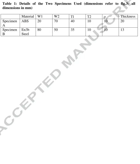
Detailed analysis and testing was carried out on two slightly different test specimens, designed to represent typical engineering components in common use such as brackets, suspension parts etc. Fig.3 shows the basic geometry and loading: a bar clamped at one end and loaded at the other to create cantilever bending, containing two equal and opposite 90o fillets. Failure is expected to occur due to high tensile stress in the upper
A crucial aspect of any real engineering design problem is the existence of specifications which place constraints on the design. In our case these refer in particular to the locations of points P and Q, which may be allowed to vary but only within certain limits, determined by the functionality of the component. We imposed the following constraints in this case:
(i) Point P is fixed in the x direction, and point Q is fixed in the y direction, thus keeping the overall dimensions of the part (W1, W2, T1 and T2) constant. (ii) Point P can vary in the y direction but only between y=0 and y=10mm. This
means that P cannot move up above the location that it has in the constant-radius part.
(iii) Q can vary in the x direction from 0 to W2, i.e. it can take any location within the overall dimensions of the part.
Finite element analysis was carried out using ProEngineer software: mesh refinement was employed until all solutions converged.
Approach (1): The Local Curvature Method
This section describes a new approach which we developed to allow post-processing of data from a constant-radius notch to create an improved variable-radius notch; we call this the Local Curvature Method (LCM). It is based on the idea that, whatever the geometry of the stress concentration feature, the local stress is strongly affected by the local radius of curvature of the surface. In general, increasing the radius of the notch, fillet etc will decrease Kt, but the relationship between peak stress σmax and radius
ρ depends on geometry, loading, etc. A well known relationship which applies exactly to the case of an elliptical notch in an infinite plate in tension, and gives a reasonable approximation for many other types of notches, is:
ρ
σ
σ
D nom 2 1max = +
(1)
…where σnom is the nominal applied stress (making the left hand side of the equation
equal to the stress concentration factor Kt) and D is the notch depth. Thus the peak stress
is approximately proportional to the inverse of the square root of the radius, other things being equal. We made use of this relationship to design a procedure described by the following instructions:
a) Carry out a normal FEA of the component, subjected to the expected loads and constraints in service, using a constant radius ρo between points P and Q (as
shown in fig.1).
c) Create a new curve in which the radius ρ varies with r, such that it is proportional to the square of the local stress σ. Thus the curve will conform to the following relation:
2
=
σ
σ
ρ
ρ
av oC
(2)C is a constant which ensures that the average radius is still ρo. This procedure creates a
new curve having a reduced radius in areas where the local stress was high, and increased radius in low-stress areas. A simple way to generate this curve is to specify the angle through which it turns at each of a series of points along the curve. Imagine the curve divided up into n equal intervals, giving (n+1) points Po, P1…Pn. Fig.4a shows two
adjacent points Pi and Pi+1. At point Pi the angle between the curve and the y axis is θi; the
total angle turned along the whole curve is β. Τhe change in θ on going from one point to the next, αI = θi+1- θI, is proportional to the local radius of curvature at that point.
For the case of the constant-radius notch α is constant along the curve. From our stress analysis we find the value of the local stress at each point, σi. To calculate the shape of
the variable radius notch we first calculate αi such that:
(
)
2
1 /2 + = + i i av
i n σ σ
σ β
α (3)
In general this will lead to a curve which turns through a total angle which is greater than or less than β. This problem is solved by multiplying all αI values by a constant factor so
that their sum is equal to β. The coordinates of the new points Pi making up this curve
can then be found by simple trigonometry. Assuming that the curve is made up of a series of straight lines of equal length ∆s (which will be sufficiently accurate if the number of points is large enough) then if the coordinates of point Pi are (x,y) and those of Pi+1 are
(x’, y’):
x’ = x + ∆s.sin(θi +α/2) (4)
y’ = y + ∆s.cos(θi+α/2) (5)
These calculations can easily be implemented, for example in Microsoft Excel, and take a negligible amount of time to perform. One difficulty with equation 2 is that ρ becomes very large if σ is very small, approaching infinity if the stress is zero. This can create a situation where almost all the curvature of the line is confined to one region, where the stress was originally very small. This problem can be avoided by identifying regions where the stress is much smaller than σav, (we used a cutoff value of σav/4) and resetting
One remaining problem is that the new curve will not pass through both ends of the original curve: P and Q. So in order to decide on the final location of the curve one has to consult the design constraints on these two points, as mentioned above. We can move and/or scale the curve until these design constraints are met. Scaling involves changing the overall dimensions without changing shape. In scaling the curve, if this leads to an increase in the average radius, this is expected to be a good thing, so the final curve will be chosen so as to have the largest possible average radius, within the limitations imposed by the design constraints.
Fig.4b illustrates this procedure, as implemented in the case of specimen type A. We began the analysis (arbitrarily) from point P, creating a variable-radius curve which also began at this point. Because in this case the stresses near P were relatively small, peaking at a point closer to Q, the new line showed high initial curvature, flattening out towards the end. Scaling this curve up whilst keeping one end at P was not possible because the other end would have been beyond the right hand edge of the specimen, thus violating one of the design constraints. The largest average radius was achieved by shifting the starting point down to slightly below P (y = 7.95mm), the end point now coinciding with the edge of the specimen. These manipulations, being done by hand, take some time but can be completed relatively quickly by an experienced designer. It would be possible to automate this process by writing a small piece of software to redraw the curve based on the constraints given.
The results obtained using this approach are given in Fig.5, which shows FEA contour plots for stresses in the constant-radius and variable-radius versions of specimen A, with the same applied force. It is evident that the maximum stress point has been smoothed out in the new design. The maximum value of the first principal stress was smaller in the variable-radius design by a factor of 1.8, a very considerable improvement. For specimen type B we obtained a slightly better stress reduction factor of 2.0.
Approach (2): Using modeFrontier Software
and likewise P3 requires only the x coordinate. P2 on the other hand requires 2 points, giving a total of 4 degrees of freedom in the final curve. Limitations were imposed on the point P2 in order to avoid solutions which would be obviously undesirable, such as inflection points in the curve. This allowed us to generate a wide range of different curves within the design constraints. We did investigate using more degrees of freedom, by increasing the number of control points in the Bezier curve, but we found that this only resulted in many curves which were far from optimal: probably some useful curves could be generated but only by greatly increasing the number of FE models analysed. We found using the three-point Bezier curves that a reasonable description of the design space could be achieved using 60 FE models. We felt that this was a sensible upper limit to the computation considering that, in practice, the method should be applicable to real engineering components, for which each individual run might take a considerable time.
Fig.6 shows the results obtained for specimen type B, plotted in two different ways. Each individual point on the plot represents one FE model. In fig.6a the two variables being optimized are the maximum stress and the mass of the specimen: the size of each point represents the x-coordinate of point Q (equivalent to point P3 of the Bezier curve). In fig.6b the x-coordinate of Q is plotted instead of mass, with the point size being the y-coordinate of point P. These plots illustrate the ability of the software to present data in diverse ways, seeking optimal solutions when multiple variables are present, which may be helpful to the designer. In the present example our aim was to minimize σmax within
the specified design constraints, so strictly speaking the best solution obtained is that which gives the lowest stress, since all models were constrained to stay within the specified range for points P and Q. So in this case the best solution gave a stress of 1.22MPa: this is also equal to the value of Kt as the loading was chosen to give a nominal
stress of 1MPa. For comparison, the same load applied to the constant-radius model gave a stress of 2.6MPa, thus the stress reduction factor is 2.13, somewhat larger than the factor of 2.0 which we obtained for the same specimen using the LCM above.
This approach also allows more sophisticated analysis of results, which may be appropriate in cases where the design constraints cannot be precisely stated but may be more “fuzzy” in nature. For example, as regards point Q, it may be that, whilst any value up to the specimen edge is allowable, smaller values may be more desirable. Thus, looking at fig.6b, the designer notes that a range of possible solutions exist, given by the line which defines the limit of the cloud of data points. This line is known as the Pareto Front. It gives a clear indication of the interaction between variables, in this case the trade-off between stress and the position of Q. Fig.6a, on the other hand, displays the relationship between stress and weight; in many cases this would be a crucial factor to consider, though in the present case the absolute change in weight from one model to another is small enough to be negligible.
Experimental Results
specimens of each design: the average failure load was 1.18kN for the constant-radius specimens and 2.17kN for the variable-radius specimens. The ratio between these loads, 1.84, agrees closely with the predicted improvement of 1.8.
For type B we chose one of the many designs analysed. This was not the best one in the sense of having the lowest stress, but represented a point on the Pareto curve giving a good compromise between stress reduction and dimensions. This particular design had shown an improvement (compared to the constant-radius specimen) by a factor of 1.3. Fig.7 shows the results of the fatigue tests, plotting the number of cycles to failure as a function of the applied stress range. The variable-radius design clearly gave improved fatigue behaviour, with all points lying above those obtained from the constant-radius specimens. In the case of the constant-radius specimens two tests were stopped when the specimens had not failed after 2 million cycles. We obtained an improvement in fatigue strength for the variable-radius specimens of a factor of 1.47 at 2 million cycles, which is slightly better than our predicted factor of 1.3. The improvement decreased at smaller numbers of cycles to failure, to a factor of 1.20 at 70,000 cycles. The average factor over the whole curve was 1.34, which is very close to our predicted value.
Further Examples
We reanalyzed the specimen used by Mattheck, as shown in fig.2. Mattheck’s approach was able to reduce the Kt factor to 1.15. We obtained a Kt factor of 1.08 using the LCM,
which resulted in a curve having very similar end points to those of Mattheck’s curve. Using mF we were able to reduce Kt even further, to 1.05. We also applied the LCM to
the case of a circular hole (radius 25mm) in a 100mm square plate loaded in tension along one pair of edges. In this case we were able to reduce the maximum stress by a factor of 1.6. These results were not verified experimentally.
Discussion
Previous work in this area has already demonstrated that improvements of this magnitude can be obtained. The novelty of the present work is in the demonstration of two new approaches. The Local Curvature Method, which we describe here for the first time, allows very significant improvements to be made based on a simple and rapid analysis of the constant-radius notch. The method is potentially applicable to bodies of arbitrary geometry and so could be applied to any engineering component, though some refinements would be needed in certain cases, where the notch has a more three-dimensional character. The use of modeFrontier software, here applied to this type of problem for the first time, allows a more systematic analysis to be conducted. In multi-variable problems such as this it is always difficult to prove that the solution obtained is truly optimal, in the sense of being the best possible solution. Here we have shown that the mF software could generate solutions which were slightly better than those obtained by our LCM and by the approach of Mattheck, though admittedly at the cost of a much greater amount of computation time. A further advantage of the mF software is the facility to appreciate the competing effects of several variables in the context of the whole design problem for the component.
The experimental work demonstrated improvements in static strength and fatigue strength which were close to the predicted values. It should be noted that this will not always be the case. Here we chose two situations – the static failure of a brittle polymer and the high-cycle fatigue strength of a metal – for which it is known that failure is largely controlled by maximum stress, and therefore changes in Kt will be directly mirrored by
changes in component strength, provided that Kt factor is relatively small, say less than 3.
For higher Kt factors, the change in strength will be less than the change in maximum
stress in both cases, owing to stress gradient effects. Methods already exist for predicting the magnitude of these effects (see for example [8]) and these methods could be used in conjunction with the procedures described here, to estimate the likely improvements in performance for a wide range of stress concentration features and failure modes.
Conclusions
1) The effects of stress concentration features can be greatly reduced by making subtle changes to their shapes, altering local curvature to make a variable-radius notch instead of a constant-radius notch.
2) The Local Curvature Method (LCM) is capable of creating variable-radius notches with greatly reduced maximum stresses, using a very simple approach based on post-processing data from a finite element analysis of a conventional constant-radius notch. This approach could be very useful in industrial situations where there is only limited access to computing resources.
3) The modeFrontier software can be used where more extensive computing resources are available, to conduct a systematic search covering a wide range of variable-radius designs. This approach was able to find solutions which were slightly better than those of the LCM.
We are grateful to EnginSoft SpA for provision of the modeFrontier software.
Figure Captions
Figure 1. A general statement of the problem. A body (having arbitrary shape, loads and restraints) contains a constant-radius curve PQ over which the stress reaches its maximum value. The objective is to redraw this curve with a variable radius in order to reduce the maximum stress.
Figure 2. An example of the approach of Mattheck (from [5]). A specimen loaded in tension at the top edge and restrained along the bottom edge (the left hand edge is a plane of symmetry). The curve labeled “non-optimized” has a constant radius, that labeled “optimized” was created using Mattheck’s approach. The graph shows stresses measured along the surface for both designs, normalized by the applied stress.
Figure 3. Specimen geometry and loading.
Figure 4a. The curve is divided into points Pi; at each point the angle to the y axis is θi;
the angle turned between Pi and Pi+1 is αi.
Figure 4b. Illustration of the curve-drawing procedure used for the LCM. A variable radius curve is first generated which starts from P (labeled “Variable radius (original)). This curve is then scaled and moved to conform to the design constraints.
Figure 5a. Stress contours for specimen A: constant-radius
Figure 5b. Stress contours for specimen A: variable-radius
Figure 6a. Results of analysis of specimen B, showing maximum stress as a function of mass. The size of each point represents the x coordinate of point Q.
Figure 6b. Results of mF analysis of specimen B, showing maximum stress as a function of the x coordinate of point Q. The size of each point represents the y coordinate of point P.
References
1. Peterson, R. E., Stress concentration factors, Wiley 1973.
2. Grodzinski, P., "Investigations on shaft fillets," Engineering (London), Vol. 152, 1941, pp. 321-331.
3. Baud, R. V., "Beitrage zer Kenntnis der Spannungsverteilung in Prismatischen und Keilformigen Konstruktionselementen mit Querschnittsubergangen,"
Eidgenoss Materialpruf, Vol. 83, 1934.
4. Thum, A. and Bautz, W., "Der Entlastungsubergang-Gunstigste Ausbildung des Uberganges an abgesetzten Wellen," Forsch Ingwes, Vol. 6, 1934, pp. 269-277.
5. Mattheck, C., Design in Nature: Learning from Trees, Springer, Berlin, 1998.
6. Mattheck, C., Erb, D., Bethge, K., and Begemann, U., "Three-dimensional shape optimization of a bar with a rectangular hole," Fatigue and Fracture of
Engineering Materials and Structures, Vol. 15, No. 4, 1992, pp. 347-351.
7. Mattheck, C., "Teacher tree: The evolution of notch shape optimization from complex to simple," Engineering Fracture Mechanics, Vol. 73, No. 12, 2006, pp. 1732-1742.
Table 1: Details of the Two Specimens Used (dimensions refer to fig.3: all dimensions in mm)
Material W1 W2 Thickness Specimen
A
ABS 20 70 40 10 10 20
Specimen B
En3b Steel
80 50 35 10 10 13
[image:13.612.82.537.178.712.2]Research Highlights
- Two new methods for obtaining variable radius notches with reduced stress concentration factors