Segmentation by Incremental Clustering
Dao Nam Anh
Department of Information Technology
Electric Power University 235 Hoang Quoc Viet road
Hanoi, Vietnam
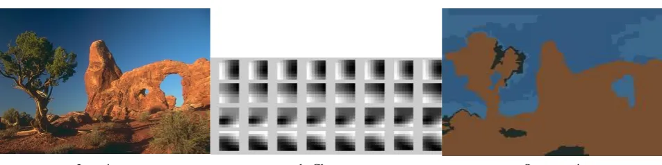
[image:1.595.60.537.169.288.2]a. Input image b. Clusters c. Segmentation
Figure 1: Segmentation by incremental clustering
ABSTRACT
A method for unsupervised segmentation by incremental clustering is introduced. Inspired by incremental approach and correlation clustering, clusters are added and refined during segmentation process. Correlation clustering is to keep away from pre-definition for number of clusters and incremental approach is to avoid re-clustering that is needed in iterative methods. The Gaussian spatial kernel is involved like a part of similarity function to cover local image structure. Cluster representative is updated efficiently to satisfy the old and new similarity constraints rather than re-clustering the entire image. Experimental results are discussed and show that the algorithm requires reasonable computational complexity while gaining a comparable or better segmentation quality than standard methods.
General Terms
Pattern Recognition, Algorithms
Keywords
Incremental Clustering, Correlation Clustering, Unsupervised Segmentation
1.
INTRODUCTION
Image segmentation refers to a field of image processing that aims to partition an image into disjoint regions. The overriding objective is to generate homogeneous regions and difference of their neighboring in respect to some characteristics such as color, intensity, or texture. Clustering approach is widely used for image segmentation. It is the search of clusters such that objects within the same cluster are similar while objects in different clusters are distinct in some feature space. Here, the clustering provides similarity measurement of image regions in segmentation process.
Interest in the image segmentation by clustering has increased significantly among the research community to the varied and important applications of segmentation. Some of the key clustering include: k-Mean [01], [02], [03], EM [04], Mean-shift [05], [06] and Graph-cut [07].
There is a popular task in clustering algorithms to pre-define the number of clusters. Inadequate pre-selection of the
number of clusters may lead to bad clustering outcome. This also may make the algorithms insufficient for batch processing of big image databases. There has been some work by Dempster et al. [08] to bridge this gap by providing the Expectation-maximization (EM) algorithm which is a general-purpose maximum likelihood algorithm for missing-data problems, has been applied to estimate the parameters of mixture models. However, speed of convergence of the EM algorithm is dependent on the amount of overlap among the mixture components and is sometimes very slow [09], [10].
Correlation clustering [11], [12] is a data mining method for clustering that does not require a bound on the number of clusters that the data is partitioned into. Thus, the method divides the data into the optimal number of clusters based on the similarity between the data points. On the other hand, incremental clustering [13], [14], [15] is approach to refine clusters dynamically.
This work continues with the incremental clustering approach, the correlation clustering, and in particular applies the approaches for image segmentation. A new incremental clustering based segmentation algorithm is presented in this paper. In the proposed method, the number of clusters is not predefined and clusters are added during clustering process. Therefore, the number of clusters is increased incrementally but it’s constrained by a max number. The distance function for similarity measurement is based on Gaussian distribution [16] to cover partially local image structure.
In fact, the proposed approach is fast, non-iterative, simple to implement. Please refer to figure 1 for an example of image segmentation by the incremental clustering algorithm. Fig. 1a shows the original image. Four clusters which are added and updated in clustering process are displayed in fig. 1b and segmentation result is demonstrated in fig. 1c.
2.
OUTLINE OF PAPER
3.
PRIOR WORK
In order to gain a better understanding of the article goals and approach it is helpful to first briefly outline some traditional segmentation clustering methods including incremental clustering.
k-Means clustering algorithm was developed by J. MacQueen [01] and then by J. A. Hartigan and M. A. Wong [02]. The method is simple and fast. It’s necessary to pick-up k - the number of clusters. Mean of each cluster from its member is re-computed. If no mean has changed more than some ε, then stop.
Fuzzy c-means clustering (FCM) [17] is more natural than hard clustering. Objects on the edges between several clusters are not forced to fully belong to one of the clusters, but rather are assigned partial membership. FCM and bilateral filter [18] is applied for image segmentation [19].
Mean shift segmentation [05], [06] is a nonparametric clustering technique, which does not require prior knowledge of the number of clusters. The mean of the data in search window is re-computed in each iteration and the search window is centered at the new mean location. Repeat this until convergence. The algorithm is calculation intensive. Graph cut segmentation [07] is a graph-based approach that makes use of efficient solutions of the max flow/mincut problem between source and sink nodes in directed graphs. This generic framework can be used with many different features and affinity formulations thought high storage requirement and time complexity.
Most clustering methods request re-calculation in feature space through iteration loops for clustering data. Incremental clustering provides a process of incremental classification that aim at refining the partial classification in an iterative way, where features are progressively evaluated [20].
An incremental clustering algorithm for data mining was developed by Ester et al. Algorithm DBSCAN in [13] is a density-based and partition clustering. Hierarchical agglomerative clustering (HAC) or Hierarchical cluster analysis (HCA) is presented in [14], [15] for cluster analysis which seeks to build a hierarchy of clusters. An incremental clustering algorithm is proposed in [21] with changing the radius threshold value dynamically. The algorithm restricts the number of the final clusters and reads the original dataset only once. Next, images in [22] can be segmented by incremental iterative clustering where a gravitational function is defined in feature space to manage clustering process.
There are some specific problems of incremental k-Means including the seeding problem, sensitivity of the algorithm to the order of the data, and the number of clusters. Static and dynamic single-pass incremental k-Means procedures are presented in [23] to overcome these limitations. Other incremental version of the k-Means algorithm is shown in [24] that involves adding cluster centers one by one as clusters are being formed. An incremental partitioning based k-Means clustering is addressed in [25]. It is applied to a dynamic database where the data may be frequently updated.
Expectation conditional maximization (ECM) [26] and α-EM algorithm [27] were developed from EM by Fraley al. [28]. These methods can be applied to estimate the number of clusters using mixture models.
4.
INCREMENTAL CLUSTERING
Given an RGB image presented by an M-dimension function of space: )) ( ),.. ( ( : ) ( ,
: u x u1 x u x
u N M , 2
x (1)
M i
ui:, 1,.., (2)
Our goal is to perform clustering the input image into clusters:
} ,.. 1 {c,j k
C j (3)
by building membership function
f
that maps pixels i x to j c C xf( i): (4)
Denote s(x)- a spatial frame of the size with center in x
... ... ... ... ... ... ... ... ... ... ... ... )
(x x
s
(5)
Mark
u
(x
)
for the extraction ofu
(x
)
in a frame of the size
with center in x ... ... ... ... ... ... ) ( ... ... ... ... ... ... )) ( ( )
(x f sx ux
u
(6)
4.1
Similarity Measurement
Given a clustersj
c and a pixel i
x, their similarity function
can be described in L-norm of difference between
(cj)and) (xi
u :
k j c x u c x
d( i, j) ( i)( j)L, 1,.. (7)
Here
(cj) is representative of cluster jc - a matrix with size
. Most clustering algorithms represent clusters by their centroid and use an Euclidean distance in building them. This may produce generally a hyper-spheric cluster shape, therefore makes them unable to obtain the real image structure [29]. The function d(xi,cj)is in Euclidean metric whenL2.In this case, all positions in the frame
with center in xare equal. So, in order to capture local image structure better, the function ( , )
j i c
x
d may involve Gaussian kernel G for spatial distance: 2 2 2 exp 2 1 ) , ( y x y x G (8)
This kernel can play weighting role for the similarity function:
) ( 1 ) ( ) ( * , 1 ) , ( i s i ysxi x
j
i G x y u y y
W c x
d
(9)
where
i
x
W is normalization factor:
G
x
,
y
Note that L1 is used in (9). The similarity function is
applied like the base of cluster assignment for pixel i x: )) , ( ( min arg : )
(xi c* C C d xi cj
f j (11)
4.2
Algorithm
The incremental clustering (IC) based segmentation algorithm proceeds by user initially selecting input image , frame size
, similarity threshold, spatial deviation
and maximum number of clustersmax
k
. Let the set of clusters empty at the beginning:C=Ø, k=0. (12)
For each xi,i1..n the algorithm takes the following steps:
Step 1. Computing the memberships: Find distance from
i
xto existing clusters by the similarity function (9, 10):
k j c x
d( i, j), 1,.. (13)
If exists cluster (k>0) and
( ( , ))
minc C d xi cj
j
then assign
membership forxi:
)) , ( ( min arg : )
(xi c* C C d xi cj
f j (14)
Else
Step 2. Add new cluster:
if number of clusterskkmax, add a new cluster to C:
1 1
1, ( ): ( ), :
j i j
j c u x C C C
c (15)
and assign membership of xito the cluster:
1 *:
)
(xi c cj
f (16)
else assign membership of i
x to cluster c*found by (14) Step 3. Updating representative for the cluster c*
1 ( ) *
*) ( )
( *
c x c
numel u x
c
(17)
where numel is short for number of elements.
Turn to step 1 until all pixels were clustered./.
Note that averaging representative by (17) requests saving historical
(cj). Rather than reserve space for this,averaging operation may have iterative form: averaging value is updated by the value of new member:
) ( ) ( ) 1 ) ( ( * ) ( : ) ( * * * * c numel x u c numel c
c
(18)
4.3
Computational Complexity
Let n is the number of pixel x. Earlier we showed that the operation (18) doesn’t require
(cj) and the IC algorithmhas space complexity (kmaxn). In case to store
(cj) by (17), the space complexity is (nlogn).Time complexity is (kmaxn). The algorithm takes as much time as big
max
,
,
k
andn. In experiments described in next section our preference for these parameters are5 , 4 , 3 , 3 ,
3 max
k
(19)5.
EXPERIMENTS
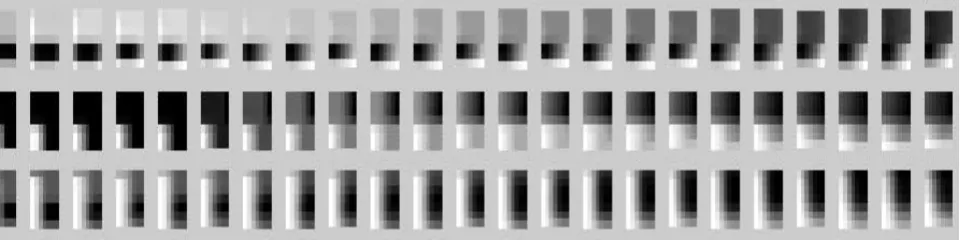
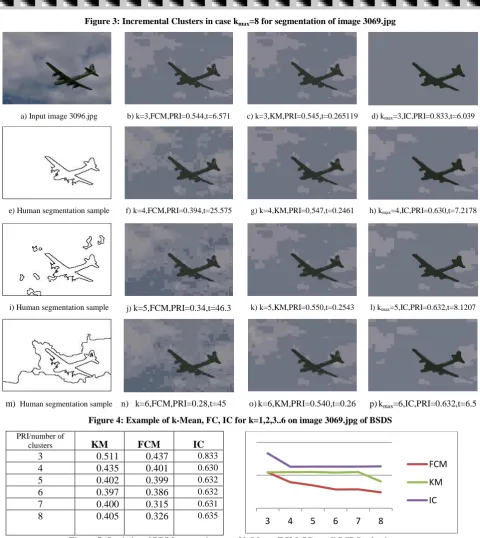
Figure 2 shows an example of cluster update in time series during clustering image 3096.jpg from BSDS500 [30] with
3
max
k . Clustering the same image withkmax 8produced historical clusters displayed in figure 3.
Probabilistic Rand Index (PRI) [31], [32] is selected for segmentation quality measurement in our experiments. Each segmentation result was compared with all three human segmentation samples and get PRI as average of RIs [31].
Figure 4 shows effect of parameter
max
k for clustering 3096.jpg. Original image is displayed in fig 3a. Human segmentation samples are shown in fig 3e, 3i, 4m. They are used like reference objects for the PRI estimation. Calculation time (t) is measured by sec (s). Segmentation by clustering for the image was performed also by k-mean [01], [02] and Fuzzy c-means clustering (FCM) [17]. IC algorithm gave the best PRI=0.833 and time t= 6.039 (fig. 4d) for kmax 3. Statistics
of PRI for image 3096.jpg is shown in figure 5.
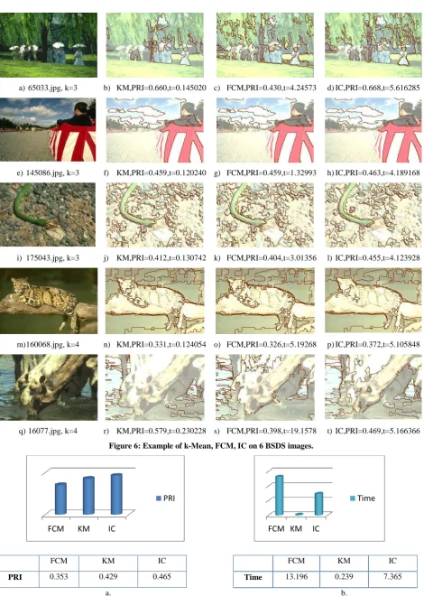
Figure 5 presents clustering results for some other BSDS images when kmax 3,4. Statistics from experiment on all
BSDS images is presented in figure 7a, where average PRI for FCM, KM, IC are 0.353, 0.429 and 0.465 accordingly. Thus, this showed that IC improved PRI, though it takes more time than k-Mean (see fig. 7b).
Figure 2: Incremental clusters in case kmax=3 for segmentation of image 3069.jpg
[image:3.595.63.544.597.717.2]Figure 3: Incremental Clusters in case kmax=8 for segmentation of image 3069.jpg
a) Input image 3096.jpg b) k=3,FCM,PRI=0.544,t=6.571 c) k=3,KM,PRI=0.545,t=0.265119 d) kmax=3,IC,PRI=0.833,t=6.039
e) Human segmentation sample f) k=4,FCM,PRI=0.394,t=25.575 g) k=4,KM,PRI=0.547,t=0.2461 h) kmax=4,IC,PRI=0.630,t=7.2178
i) Human segmentation sample j) k=5,FCM,PRI=0.34,t=46.3 k) k=5,KM,PRI=0.550,t=0.2543 l) kmax=5,IC,PRI=0.632,t=8.1207
m) Human segmentation sample n) k=6,FCM,PRI=0.28,t=45 o)k=6,KM,PRI=0.540,t=0.26 p)kmax=6,IC,PRI=0.632,t=6.5
Figure 4: Example of k-Mean, FC, IC for k=1,2,3..6 on image 3069.jpg of BSDS
PRI/number of
clusters KM FCM IC
3 0.511 0.437 0.833 4 0.435 0.401 0.630 5 0.402 0.399 0.632 6 0.397 0.386 0.632 7 0.400 0.315 0.631 8 0.405 0.326 0.635
3 4 5 6 7 8
[image:4.595.57.538.217.756.2]a)65033.jpg, k=3 b) KM,PRI=0.660,t=0.145020 c) FCM,PRI=0.430,t=4.24573 d)IC,PRI=0.668,t=5.616285
e)145086.jpg, k=3 f) KM,PRI=0.459,t=0.120240 g) FCM,PRI=0.459,t=1.32993 h)IC,PRI=0.463,t=4.189168
i) 175043.jpg, k=3 j) KM,PRI=0.412,t=0.130742 k) FCM,PRI=0.404,t=3.01356 l)IC,PRI=0.455,t=4.123928
m)160068.jpg, k=4 n) KM,PRI=0.331,t=0.124054 o) FCM,PRI=0.326,t=5.19268 p)IC,PRI=0.372,t=5.105848
[image:5.595.63.534.58.719.2]q)16077.jpg, k=4 r) KM,PRI=0.579,t=0.230228 s) FCM,PRI=0.398,t=19.1578 t)IC,PRI=0.469,t=5.166366
Figure 6: Example of k-Mean, FCM, IC on 6 BSDS images.
FCM KM IC FCM KM IC
PRI 0.353 0.429 0.465 Time 13.196 0.239 7.365
a. b.
Figure 7: PRI and Time Complexity by FCM, KM and IC from BSDS experiments.
FCM KM IC
PRI
FCM KM IC
6.
DISCUSSION
The IC algorithm does clustering incrementally by only one round of checking pixels of input image. As similarity function works on
-size frame, it takes more time than k-Mean. In order to have the best representative frame for cluster, the frame must be full size. It means that pixels inside input image having full neighbours for the
-size frame should be considered first to create all necessary cluster representatives. Other pixels laying on borders of input images will be checked later, just for membership assignment. As big as spatial deviation
and frame size
, the local structure is considered in similarity function, but gets more computing time. Our practical preference for
and
is 3.The similarity threshold has close association to the final number of clustersk. As less, clusters are added as more frequently and final number of clusters reaches as quickly the
max
k . So the similarity threshold may be taken from experimental statistics for optimal solution.
7.
FUTURE WORK
The need for similarity measurement is essential for segmentation by clustering. Though IC method utilizes local neighborhood information in the measurement but some parameter selection requires specific consideration for better result. Fuzzy set [17] could be a solution for getting solution for the case and it may help to ameliorate clustering process.
8.
CONCLUSION
In this paper, aiming at producing image segmentation, a new algorithm is proposed to generate clusters incrementally. Similarity function with Gaussian spatial kernel is applied to manage membership assignment. Clusters are created due to necessary and cluster representative is updated every time when having a new member for a cluster. Our algorithm is a fully automatic method with optional parameter selection for more flexibility. The algorithm works well on various examples. A careful evaluation by statistics on BSDS shown that algorithm requires reasonable computational complexity while gaining a comparable or better segmentation quality than standard methods.
9.
ACKNOWLEDGMENTS
Author thank Berkeley Computer Vision group for the BSDB, its images were used in experiments of this article. Author would also like to thank the anonymous referees for their careful review and constructive comments.
The article was supported by the 2015 e-Library Project of the Electric Power University and the results of the article are applied for images processing for the e-Library documents.
10.
REFERENCES
[1] J. MacQueen, Some Methods for Classification and Analysis of Multivariate Data, Proc. 5th Berkeley Symposium on Probability and Statistics, May 1967.
[2] J. A. Hartigan and M. A. Wong, Algorithm AS 136: A k-means clustering algorithm, Applied Statistics, vol. 28, no. 1, pp. 100–108, 1979.
[3] R.O. Duda, P.E. Hart, Pattern Classification and Scene Analysis, Wiley, Toronto, 1973.
[4] Bishop, Christopher M. (2006). Pattern Recognition and Machine Learning. Springer. ISBN 0-387-31073-8.
[5] Cheng, Yizong (August 1995). Mean Shift, Mode Seeking, and Clustering. IEEE Transactions on Pattern Analysis and Machine Intelligence (IEEE) 17 (8): 790– 799. doi:10.1109/34.400568.
[6] D. Comaniciu and P. Meer. Mean shift: A robust approach toward feature space analysis. IEEE Trans. Pattern Anal. Machine Intell., 24:603–619, 2002.
[7] D.M. Greig, B.T. Porteous and A.H. Seheult (1989), Exact maximum a posteriori estimation for binary images, Journal of the Royal Statistical Society Series B, 51, 271–279.
[8] Dempster, A.P.; Laird, N.M.; Rubin, D.B. (1977). Maximum Likelihood from Incomplete Data via the EM Algorithm. Journal of the Royal Statistical Society, Series B 39 (1): 1–38. JSTOR 2984875. MR 0501537.
[9] C. F. Jeff Wu, On the Convergence Properties of the EM Algorithm, The Annals of Statistics, Vol. 11, No. 1 1983, pp. 95-103.
[10] Vaida F. Parameter convergence for EM and MM algorithms. Statistica Sinica 2005; 15:831-840.
[11] Nikhil Bansal, Avrim Blum, and Shuchi Chawla. Correlation clustering. In Proceedings of the 43rd Annual IEEE SFCS, pp 238250, 2002.
[12] Becker, H. A survey of correlation clustering. Available online at www.cs.columbia.edu/~hila/clustering.pdf, 2005.
[13] Ester M., Kriegel H.-P., Sander J., Xu X.: Incremental Clustering for Mining in a Data Warehousing Environment, Proc. 24th Int. Conf. on Very Large Databases (VLDB ‘98), New York City, NY, 1998, pp. 323-333.
[14] R. Sibson (1973). SLINK: an optimally efficient algorithm for the single-link cluster method. The Computer Journal (British Computer Society) 16 (1): 30– 34. doi:10.1093/comjnl/16.1.30.
[15] M. Charikar, C. Chekuri, T. Feder, and R. Motwani. Incremental clustering and dynamic information retrieval. In The 29th annual ACM symposium on Theory of computing, pp 626–635, 1997.
[16] M. Lindenbaum, M. Fischer, and A. M. Bruckstein, On Gabor’s contribution to image enhancement, Pattern Recognition, 27 (1994), pp. 1–8.
[17] Dunn, J.C.: A Fuzzy Relative of the ISODATA Process and its Use in Detecting Compact Well Separated Clusters. Jour. of Cybernetics, Vol. 3, 1974, pp. 32–57.
[18] C. Tomasi and R. Manduchi. Bilateral filtering for gray and color images. In Proc. of the Sixth International Conference on Computer Vision, India, 1998.
[19] Kai X, Jianli L, Shuangjiu X, Haibing G, Fang F and A E Hassanien, Fuzzy Clustering with Multi-Resolution Bilateral Filtering for Medical Image Segmentation, (IJFSA), Vol3, Issue 4. 2013. 13 pp.
[20] Guillaume B, M Verleysen, John A. Lee, Incremental feature computation and classification for image segmentation, ESANN 2012, ISBN 978-2-87419-049-0.
2009 (ISIP’09) ISBN 952-5726-02-2 (Print), 978-952-5726-03-9, 2009, pp. 175-178.
[22]Rashedi, E.; Nezamabadi-Pour, H. A Stochastic Gravitational Approach To Color Image Segmentation By Considering Spatial Information Engineering Applications Of Artificial Intelligence, V26, N4, 2013.
[23]Aaron, B.;Tamir, D.E.; Rishe, N.D.; Kandel, A. Dynamic Incremental k-Means Clustering, (CSCI), 2014 (Vol:1), DOI: 10.1109/CSCI.2014.60.
[24]Pham, Duc Truong, Dimov, Stefan Simeonov and Nguyen, C. D. 2004. An incremental k-Means algorithm. Proceedings of the Institution of Mechanical Engineers, Part C: Journal of Mechanical Engineering Science 218 (7), pp. 783-795. 10.1243/0954406041319509.
[25]Sanjay Chakraborty, N. K. Nagwani, Analysis and Study of Incremental K-Means Clustering Algorithm, High Performance Architecture and Grid Computing Communications in Computer and Information Science Vol 169, 2011, pp 338-341.
[26]Meng, Xiao-Li; Rubin, Donald B. (1993). Maximum likelihood estimation via the ECM algorithm: A general framework. Biometrika 80 (2): 267–278. doi:10.1093/biomet/80.2.267. MR 1243503.
[27] Hunter DR and Lange K (2004), A Tutorial on MM Algorithms, The American Statistician, 58: 30-37.
[28] Chris Fraley, Adrian E. Raftery, How many clusters? Which clustering method? Answers via model-based cluster analysis, The Computer Journal, 20:270–281, 1998.
[29] P. Lambert, H. Grecu, A quick and coarse color image segmentation, DOI: 10.1109/ ICIP.2003.1247125 Conference: Image Processing, 2003. Vol. 1.
[30] D. Martin and C. Fowlkes and D. Tal and J. Malik, A Database of Human Segmented Natural Images and its Application to Evaluating Segmentation Algorithms and Measuring Ecological Statistics, Proc. 8th Int'l Conf. Computer Vision, 2001, vol.2, pp 416—423.
[31] W. M. Rand (1971). Objective criteria for the evaluation of clustering methods. Journal ASA 66 (336): 846–850. doi:10.2307/2284239. JSTOR 2284239.