The application of self-tuning control to rolling mill
systems.
GROVES, Christopher N.
Available from Sheffield Hallam University Research Archive (SHURA) at:
http://shura.shu.ac.uk/19733/
This document is the author deposited version. You are advised to consult the
publisher's version if you wish to cite from it.
Published version
GROVES, Christopher N. (1993). The application of self-tuning control to rolling mill
systems. Masters, Sheffield Hallam University (United Kingdom)..
Copyright and re-use policy
See
http://shura.shu.ac.uk/information.html
101 381 062 7
Fines are charged at 50p per hour
ProQuest Number: 10697035
All rights reserved
INFORMATION TO ALL USERS
The quality of this reproduction is dependent upon the quality of the copy submitted.
In the unlikely event that the author did not send a com plete manuscript and there are missing pages, these will be noted. Also, if material had to be removed,
a note will indicate the deletion.
uest
ProQuest 10697035
Published by ProQuest LLC(2017). Copyright of the Dissertation is held by the Author.
All rights reserved.
This work is protected against unauthorized copying under Title 17, United States C ode Microform Edition © ProQuest LLC.
ProQuest LLC.
789 East Eisenhower Parkway P.O. Box 1346
The Application of Self-Tuning Control
to Rolling Mill Systems
Christopher Nigel Groves
A Thesis Submitted in Partial Fulfilment of
the Requirements of
Sheffield Hallam University
for the Degree of Master of Philosophy
May 1993
Abstract
The introduction o f self-tuning control techniques to the Automatic Gauge Control (AGC) system o f a rolling mill is considered. This is a new application o f pole-placement self-tuning control and no comparable examples have been found in the literature.
Initially, an existing ACSL model was investigated and a simpler version, suitable for on line use was developed. A simpler MATLAB model o f the system was also produced.
A data logging exercise was then carried out to allow PRBS testing and provide data for model validation. System identification and correlation analysis were then used to obtain a simplified parametric model. Included in this stage was a thorough investigation into the practical aspects o f the PRBS method for system identification and the requirements for successful implementation noted.
Acknowledgements
This project was carried out under a Teaching Company Scheme between Sheffield
Hallam University (SHU) and Davy International Sheffield. I am extremely grateful for
the assistance given to me by these three organisations and for that provided by Dr. K.
Table of contents
Abstract i
Acknowledgements ii
Table o f contents iii
1.0 INTRODU CTIO N 1
1.1 Background (History) 1
1.2 Adaptive schemes 2
1.2.1 Estimation 3
1.2.2 Design 4
1.3 Automatic Gauge Control (AGC) 4
1.4 Project Objectives 7
1.5 Major Contributions 7
2.0 M OD ELLING OF SINGLE A STAND COLD REVERSING MILL 9
2.1 The ACSL mill model 10
2.1.1 Enhancements and simplifications 11
2.1.2 Model structure 21
2.2 The MATLAB model 22
2.3 Conclusions 25
3.0 DATA ACQUISITION AND SYSTEM IDENTIFICATION 26
3.1 System Identification Options 26
3.1.1 Correlation Analysis ' 27
3.1.2 Parametric Estimation 27
3.2 Data Acquisition 29
3.2.1 Plant Data 29
3.2.2 Test Rig 34
3.3 Identification 34
3.3.1 Discussion 34
3.3.2 Algorithm Development 36
3.4 Discussion of findings 37
3.5 Conclusions 44
4.0 CONTROLLER DESIGN 45
4.1 Background 45
4.2 Options 45
4.3 Pole Placement Design 46
4.3.1 Simulations 48
4.3.2 Location of the other poles 50
4.4 Discussion 53
4.5 Conclusions 54
5.0 CONCLUSIONS AND RECOM M ENDATIONS 55
5.1 Conclusions 55
5.2 Recommendations for further work 55
APPENDIX A - ACSL code
I
A1 - Simplified drive model
I
A2 - Simplified winder model
II
APPENDIX B-MATLAB code
IV
B 1 - Code for building model
IV
B2 - PRBS generator
IV
B3 - Correlation function
V
B4 - Single step extended least squares
VI
B5 - Comparison of matrix inversion algorithms and UD
VI
factorisation
B6 - Pole-placement controller synthesis
VEH
B7 - Kucera’s algorithm
IX
B8 - Self-tuning controller
XI
APPENDIX C - C code
XIV
Cl - PRBS generator
XIV
C2 - Least squares estimation
XVII
APPENDIX D - Data logging details
XXII
APPENDIX E - Test rig details
XXHI
1.0 IN T R O D U C T IO N
This project was carried out in collaboration with Davy International Sheffield who
supply manufacturing and processing equipment to the worlds metals industries. One o f
their main areas o f expertise is Automatic Gauge Control (AGC) systems applied to
rolling mills. As a result o f Davy completing a program to develop a DDC (Direct Digital
Control) system, the foundations existed on which to develop a more sophisticated
controller. The current DDC basically does the same job as an analogue system and as
such, has no real advantages over the old analogue loops, except that the problem o f
drifting signals is removed and it is easier to log data from the digital system. Some form
o f adaptive control would hopefully tackle non-linearities and reduce the time spent on
commissioning. In addition to these benefits, such a system would also improve control
over a wide range of materials.
1.1 Background
(Hist
p i t)Processes have been controlled by conventional Proportional plus Integral plus
Derivative (PID) [1,2,3] controllers for over half a century [4,5]. This strategy has
remained unchanged despite the introduction o f microprocessor based control systems.
However, the control calculations involved in a microprocessor implementation o f a PID
controller algorithm are fairly trivial [6], With an increase in computer pow er and a
decrease in costs, the next step was to provide further features. Although it is generally
recognised that the conventional PID controller is very effective, in practice its initial
tuning and any subsequent tuning on a plant with many control loops can be very time
consuming. The effectiveness o f a PID controller is also reduced on plants with varying
parameters. Therefore one obvious method for improvement was to provide self-tuning
and adaptive capabilities [7,8,9,10],
A self-tuning controller has the ability to calculate its own control parameters, assumed
unknown but constant, at the time o f commissioning. An adaptive controller extends this
concept by altering its control parameters on-line to suit changing process conditions.
These two ideas are virtually the same, incorporating similar estimation algorithms, see
section 1.2.1 below. Potential candidates for the application o f adaptive control are
processes that are non-linear and stochastic, thus, they are difficult to analyse and
control. If they were linear they could be controlled by classical linear controllers. If they
were not stochastic or uncertain in some way there would be no requirement to learn in
the form o f self adjustment or coefficient estimation. There are no general design
procedures for non-linear stochastic processes.
Adaptive control theory has been developed over the last twenty years and several
thousand papers have been written [11,12,13,14]. Although there appears to be a great
number o f practical applications for such techniques, and developments in computer
technology have resulted in making implementation o f the algorithms possible, the
number o f successful applications actually reported is very limited. The main reason for
this is that much of the information, for competitive reasons, is kept “in-house” thus,
specific details remain unpublished.
1.2 Adaptive schemes
Three classes o f theoretical adaptive controllers exist [15,16]:
In a gain scheduling controller the designer makes use o f his knowledge o f the process
non-linearities to develop a schedule for the controller gain (plus derivative and integral
gains as required). The schedules are then used to program the controller coefficients as
a function o f one or more o f the process variables. Gain scheduling is an open loop
compensation and can be thought o f as a feedback control system in which the gains are
In model reference adaptive control systems [17] the user defines at the outset, the
closed loop system response. The desired response to set point changes is expressed in
mathematical terms and then implemented as a dynamic model. The model is subjected to
the actual set point changes and calculates in real time, the corresponding idealised
output. Within the model reference system is a conventional feedback controller with
adjustable coefficients. The process and model outputs are compared and the differences
are used to adjust the coefficients o f the feedback controller.
The two schemes above are known as implicit (or direct) methods because the
adjustment rules tell directly how the controller parameters should be updated. A
different scheme is obtained if the process model is updated and then the updated
controller coefficients are obtained from the solution o f a design problem, this is often
termed an explicit method. A self-tuning controller uses a highly simplified and linear
mathematical model o f the process. The technique uses a feedback control system
together with an identification system which continually monitors the process inputs and
outputs to produce a mathematical representation o f the process dynamics. This model is
in the form o f a generalised equation with a finite number o f parameters which are
estimated recursively. The model is then used to calculate the coefficients o f the
controller based on a defined performance requirement. Thus, there are two separate
functions being carried out, the first is a learning process (model generation) and the
second is the actual control o f its behaviour [15], It is useful at this stage to provide brief
details o f the methods available for each function.
1.2.1 Estimation
In adaptive controllers observations of the system input and output signals are obtained
sequentially in real time. It is desirable to make calculations recursively in order to save
computation time [10], The algorithms are therefore arranged in such a way that the
results already obtained can be used to obtain the new estimate o f the current dynamics
o f the process.
The most commonly used family o f algorithms is that o f least squares [11,18,19] as they
are easy to program and work well. If the same input is applied to both the system and
the mathematical model the outputs can be compared, giving rise to an error which is
dependent on how poor the estimates are. This gives an indication o f how close the
model is to the actual system. In an attempt to obtain a better model, the sum o f the
squares o f the errors is minimised by the adjustment o f the model parameters.
1.2.2 Design
Self-tuning controllers are flexible with respect to a design method. Virtually any design
technique can be accommodated. Minimum variance control is especially useful in the
design o f regulators which maintain an output value constant despite process
disturbances. It is most effective when the process is not changing. The main
disadvantage o f this method is that it does not perform well when the set point is being
varied.
A simple and direct design procedure is that o f pole placement. The objective here is to
locate the closed loop system poles at pre specified locations in order to obtain the
desired response. Designs based on gain and phase margins and on linear quadratic
Gaussian control have also been developed [15,16],
1.3 A utom atic G auge Control (A G C ) [20,21]
tolerances, increased rolling speeds for higher productivity and to reduce “off-gauge”
material, that would be scrapped or need re-working.
— hack up roll
strip.
J chock | /
/
hydraulic capsule
Side View End View
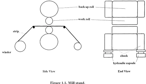
Figure 1.1, Mill stand.
The system in question is a single stand cold reversing mill which uses fast acting
hydraulic cylinders or capsules for roll adjustment. Figure 1.1 shows the mill stand
configuration, consisting of, a pay-off winder, two work rolls, two back up rolls and a
take-up winder. The back up rolls are housed in chocks (as are the work rolls normally)
and the hydraulic cylinders are placed between these chocks and the stand housings on
either side o f the mill, also see section 3.2.2.
Before rolling can begin, the mill must be threaded. This involves slowly taking strip off
the pay-off winder and passing it through the mill between the work rolls, to the take-up
winder. The mill is now set up to roll the strip which will be carried out at a greater
speed. Almost the full length o f strip is then passed between the work rolls, set to give
the required gauge reduction, leaving the mill threaded and the end o f the strip in what
was the pay-off winder. The gap between the work rolls is then reduced further and the
process repeated in the reverse direction. For operational purposes the number o f passes
[image:13.618.68.538.92.361.2]control system of which the AGC is only a part. In the roll gap, the metal is plastically
elongated in the direction of rolling. As the strip passes between the work rolls it speeds
up, thus, the strip speed is quicker on the exit side of the mill.
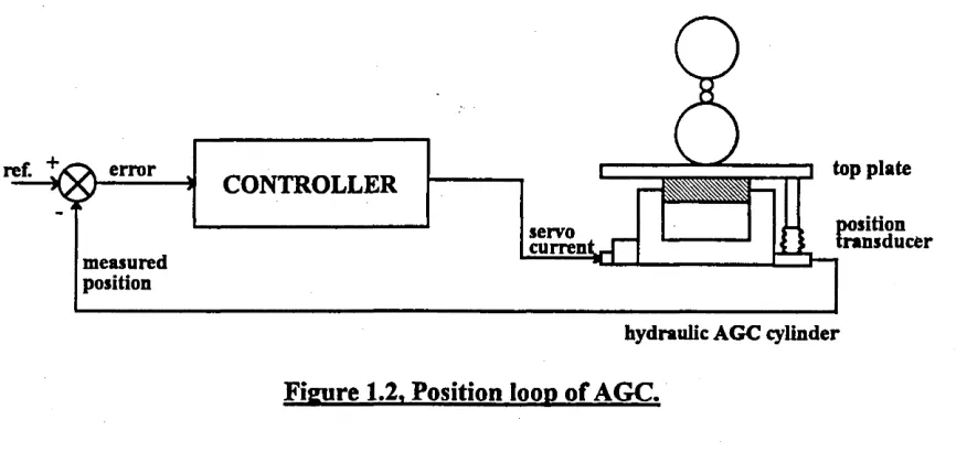
The control objective of the AGC system is to ensure minimal variation in out going strip
thickness, which is controlled by varying the gap between the work rolls. Such a system
uses one basic mode of control around the hydraulic capsules, either position control or
load (pressure) control. Other more complex control loops produce trims which adjust
the reference to the basic loop. For example, the out going strip thickness can be easily
measured and this value fed back for comparison with the desired thickness. However,
the thickness can only be measured “down stream” of the roll gap which leads to a
transport delay. As a result such measurements can only be used as slow trims, leaving
the major control effort to the fast acting position or load control loop around the
capsule. A simple extension to this principle is to fit a thickness measuring device to the
entry side of the mill and thus allow the control system to anticipate errors before the
strip enters the roll gap and correct them using feedforward control.
top plate
ref. error
CONTROLLER
position transducer servo
currenl measured
position
hydraulic AGC cylinder
Figure 1.2, Position loop of AGC.
[image:14.614.69.507.437.647.2]gauge are tension, entry gauge disturbances, material hardness changes and roll
eccentricity. In general, only proportional control is used. The servo valve and hydraulic
cylinder provide a natural integrator. Flow is proportional to input current and flow
integrates to give a load change. An additional integral term may sometimes be added to
remove any remaining steady state errors. In general, load control loops are more
difficult to stabilise than position loops.
1.4 Project Objectives
The overall aim of the project is to investigate some form of adaptive control for an
hydraulic AGC system applied to a single stand cold reversing mill. Initially, effort will
be directed towards self-tuning and will only be concerned with the position loop
controlling the hydraulic capsules. The response of this loop is well defined and the loop
can be modelled relatively easily from its basic components. If successful, the
development of an adaptive system should:
• reduce commissioning time
• improve control over a wide range of materials
• be a selling point
• allow re-tuning by the mill operator.
A further advantage is that the lessons learnt and algorithms developed here could be
applied to other loops and systems at a later stage.
1.5 Major Contributions
This is a new application and the proposed control technique has been shown to be
possible through extensive simulation studies; in addition, no comparable applications
have been found in the literature. In addition to the simulation work, logging of plant
2.0 MODELLING OF A SINGLE STAND COLD REVERSING
MILL
The suggested self-tuning controller of chapter one requires a simplified, linear model of
the system to be controlled. In addition to this model, a more complex model would be
extremely useful in the development stage for simulating the controller’s response. The
difficulty in building a mathematical model is balancing two opposing factors; including
all the relevant factors affecting system response and minimising computing time. The
question of overall accuracy must also be answered, ie what are the “relevant factors”?
These problems are obviously amplified under the constraints of real time computing.
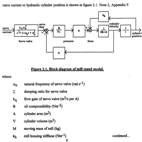
A block diagram of a simple mill stand model based on physical elements, relating servo
valve current to hydraulic cylinder position is shown in figure 2.1. Note 2, Appendix F.
cylinder velocity servo
flow servo
current cylinder
position force
Servo valve pressure
[image:17.628.74.536.302.764.2]Vs
Figure 2.1. Block diagram of mill stand model.
where:
G)n natural frequency of servo valve (rad.s’*)
£
damping ratio for servo valve
kq
flow gain of servo valve (m^/s per A)
B
oil compressibility (Nm"2)
A
cylinder area (m^)
V
cylinder volume (m^)
M
moving mass of mill (kg)
d d a m p in g term = 2 . p .V ( k |1.M ) ( p = d a m p in g factor - . 1 )
The servo valve is represented by a second order transfer function, with natural
frequency con, damping ratio C, and gain kq. The output o f the servo valve is oil flow to
the hydraulic cylinder. Flow into the cylinder will obviously be affected by any movement
o f the ram, altering the available volume and hence the pressure. The flow is integrated
to give the pressure change and thus, a change in the force acting on the ram. This force
is also dependent on the ram ’s current position. The actual cylinder is then represented
by a first order transfer function with the force acting on the ram as the input producing
a movement. This cylinder model contains a damping term, d, which is calculated from
the mill housing stiffness, the moving mass o f the mill and a damping factor, p, to
produce the required response.
2.1 The ACSL mill model
The ACSL (Advanced Continuous Simulation Language) [23] mill model is a computer
model o f a rolling mill designed for the simulation and testing o f gauge control systems.
This model was developed and used previously by Davy. The model is two dimensional
in the sense that it does not consider variations across the roll bite. A complete mill stand
model can be constructed from basic blocks, or modules, that include, mill stand with
hydraulic capsule, main motor drive with speed control and pay-off and take-up winders.
Each block being a complex non-linear ACSL model o f that particular component.
In order to understand the principles involved, a mill model was constructed by
connecting together the major modules. Once initialised, the model ran satisfactorily.
However, difficulties were experienced in maintaining tension between the roll bite and
2.1.1 E nhancem ents and simplifications
The existing model was found to be extremely complex and slow in execution and so not
suitable for any real time simulations that may be required later. The electrical drive
modules were particularly detailed and were used in three sections o f the overall mill
stand model: in the main drive and in both the pay-off and take-up winders. Thus, any
improvements made here would be amplified.
The main drive system was isolated as an ACSL model with two inputs (rolling torque
and reference speed) and one output (roll speed). A frequency response and a number of
step tests were carried out on the model in order to understand its operation. These
results would also act as a reference when testing any alterations. Throughout the tests
the armature voltage was monitored for saturation which would introduce a non linearity
into the system.
The step responses were found to be basically second order. For small steps, up to base
speed, a second order model was fitted, working with percentage overshoot and time to
cross final value. It was assumed that by alteration o f the gain at higher speeds and loads,
a similar response would be obtained, and that this was representative o f real drive
control systems. To remove any steady state error between the reference speed and the
actual speed an integral term was added to the proportional controller and a provision
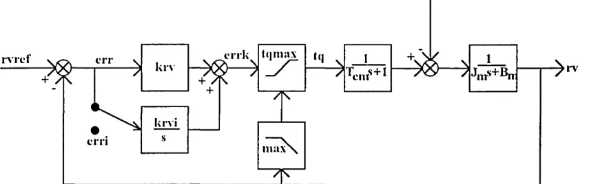
made to avoid integral wind-up. Figure 2.2 shows the block diagram for the simplified
drive model.
errk err IvIV
rv
krvi
erri max
[image:20.614.72.506.42.176.2]7T\
Figure 2.2, Simplified drive model
where:
rvref speed reference (rad.s"^)
rtq rolling torque (Nm)
rv mill speed (rad.s"l)
Jm moment ot inertia (kgm-)
Bm Damping coefficient (5% o f max. torque)
krv torque speed gain (Nm/rad.s- ^)
krvi integral gain (Nm.rad- ^)
tqmax maximum torque (Nm) (dependent on speed)
Tern time constant (s)
The system has two inputs, reference speed, rvref and rolling torque (load), rtq, and one
output, mill speed, rv. The difference between the actual speed and the reference
produces an error, err, for the proportional plus integral controller to give the control
signal, errk (the term erri is used in the prevention o f integral wind-up). The maximum
torque o f the motor, tqmax, is limited by the m otor’s speed, so the value o f tqmax is
altered as the motor speed changes once it is greater than the base speed o f the motor. A
lag term is introduced to provide a phase lag between a speed change and a torque
The response o f the modified drive model to a step in reference speed o f amplitude o f
.05 rad.s"!, from an initial speed o f 5 rad.s~l, (approximately the base speed o f the
m otor being modelled) is shown in figure 2.3. Figures 2.4 and 2.5 also show step
responses o f the modified drive model, in both cases the amplitude o f the step is much
greater, 5 rad.s'l. Figure 2.4 shows the step from 5 rad.s"! to 10 rad.s"^ and figure 2.5 a
similar step but from a much greater initial speed o f 30 rad.s’ l. These two responses
although unrealistic, (a ramp would be more appropriate for larger changes in speed),
clearly show the effect o f torque available for acceleration limiting the m otor’s speed
response.
The other area for improvement was the complete winder models. Although there are
two separate models, they are basically the same. The winders are used to pay out the
metal strip in to the mill for rolling and to coil the strip after its gauge has been reduced.
As above, the ACSL code was isolated (the take-up reel was used). On investigation this
model was found to be very oscillatory and almost impossible to set up as a stand alone
model. It was therefore decided to start again. The major problem in modelling this
system was where to introduce damping. It is not known where exactly the damping
comes from in the actual system. Two methods were investigated; damping as a result o f
frictional and other forces acting on the winder against the direction o f rotation, and
damping as a result o f the tension within the strip. Another major problem is that o f
inertia. Obviously, as a winder pays-off or takes-up strip its radius and therefore its
moment o f inertia alters.
A model was built which included a damping term based on the tension o f the strip,
figure 2.6.
90
*5
co
o
COo
o
Tt-o
rOOo
CM mto ~o c
o
o <D CO s-/ ©E
4) Vi C o Q Vi © U D v •a©E
4)> *n•o•a
c o S c« CO fS o ' u 5 WCO 00 o CO o d co o> T-" Of) •o c oo ©0) ©
E
© c/j eo Q C/3 © J. D © © T3oE
© ‘u •a T3© JC"5
E
X Tt c4 © ua
W(s/pDj) poods
CO
O
co
x>c
o
o<D
CO
©
E
ocn E O B C/i
V L.
B
V
<u
■a
oE
4)*U T3
•a
© c ’HS 35 r
in ri
(U uB W
FTREF FT
/K
rotational speed torque
A T Q
on force
[image:25.620.113.450.37.208.2]stress G.VV
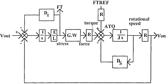
Figure 2.6, Simplified winder model block diagram.
where:
Vout speed out o f mill (m.s- ^)
FTREF Ref. tension force (N)
Von speed onto winder (m.s“l) (winder peripheral speed)
FT Front tension (N.m"-)
E Y oung’s modulus (Nm--)
L stand-winder distance (m)
Dt tension damping term (ms"^/Nm"2)
G gauge out of stand (m)
W width out o f stand (m)
R coil radius (m)
J moment o f inertia o f coil and motor (kgm2)
Ds speed damping term (Nm/rad.s- ^)
ATQ accelerating torque (Nm)
The aim o f the above model is to relate two linear speeds, the speed out o f (or in to) the
mill and the speed on to (or off) the winder. The difference between the two speeds
integrated with respect to time gives AL, which when converted to a strain and
multiplied by Young’s modulus gives the tension within the strip. This tension is then
easily converted to a torque acting on the winder. This torque is only valid in one
direction, ie the strip will not push the winder round, it will only act to oppose the
winder drive. Thus, figure 2.6 requires the addition on a non-linear block before the
summation to calculate ATQ. The mill operator will have set a desired tension in the
strip, FTREF, there will therefore be a resultant torque attempting to prevent the winder
from turning. Integration of the resulting acceleration leads to the rotational speed. The
major problem with this model is deciding where damping is introduced in to the system.
It was decided to introduce a damping term based on the tension in the strip as a result
of the speed difference between winder and mill stand. As the model stands, the
alteration in moment of inertia of each winder as strip passes through the mill is not
taken in to account.
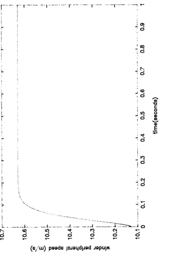
Figure 2.7 shows the response of the take-up winder peripheral speed to a step change in
strip exit speed from the roll gap. The response is highly damped, giving no overshoot
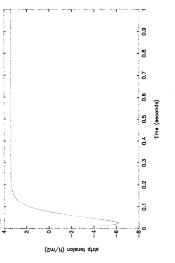
and has a rise time of approximately 75ms. Figure 2.8 shows the corresponding variation
in strip tension. The strip becomes “slack” while the winder speeds up to maintain the
required tension in strip. The strip becomes “slack” because the strip is leaving the roll
gap much quicker than it is being coiled. The tension in the strip is recovered as the
winder speed increases. It should be noted that the linear speed of the strip onto the
winder is slightly greater than the speed out of the mill, this difference is needed to
maintain the required tension. The damped response is highly desirable as any oscillation
could alter the exit gauge by drawing the metal out of the roll gap.
' 00 • ! ° t
N 1 o
©
E
J
1 o i j
j
n
■ <N 1 ot
\ i
'■'-' v " o
-I--- _4____
___I
--- ---- —i
— ---L
-o
to
to
-*
ro
<N
T—
o
o
o
o
o
o
*
— r —,
— T“*
(
s/
uj)
poods jDJoqduod jopuiM
[image:27.617.80.434.132.637.2]- i
O
o
00
! CO
1 o ^(0
■O
; c
j
o
j « s
! O coto
o
cm
o
~ i --- 1________ i_ ---r . — j________ i o
CM O CM CO 00
1 1 1 1
(Z U J /N ) U 018U 8) d p }8
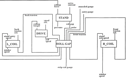
[image:28.613.63.414.122.650.2]2.1.2 Model structure
Although considerable simplifications have been made, the overall mill stand model
remains fairly complex. Figure 2.9 attempts to show all the interactions taking place in
the mill stand model by showing the individual modules and the interactions between
them. In general the data flows from top to bottom. At the centre o f the model is the
actual roll gap where the strip gauge is reduced, the actual distance between the work
rolls being determined by the servo valves in the stand model.
fro n t tension rtf . Stllllll
exit speed
DRIVE
L COIL ROLL C AP
STAND
R COIL
[image:29.614.72.492.220.480.2]w in d er speed
Figure 2.9. The structure of the complete mill stand model.
The stand module represents a mill stand with a bottom mounted capsule. The top rolls
and the top o f the mill housing are assumed to move together as one mass. As detailed
above, the servo valve dynamics are represented as a second order transfer function. The
model also takes in to account mill housing stretch and known non-linearities such as
hysteresis in the capsule and limiting o f the servo valve spool travel. L_COIL and
R_COIL represent the left and right hand winder models respectively. Figure 2.9 is
drawn for strip being rolled from left to right.
The roll gap module uses a FORTRAN subroutine to calculate rolling load, rolling
torque, deformed roll radius and forward slip [24]. The annealed gauge is used to
introduce a hardness variable into the model. The main output o f this module is the strip
exit gauge. As stated earlier, the major factor affecting winder speed is tension. The
tension within the strip also has an effect on the exit gauge. If tensions are high, the strip
is drawn plastically out o f the mill, thus giving a thinner gauge than would be expected
from the rolling load alone.
2.2 T he M A T L A B model
As mentioned above, the model required tailoring to a specific mill, so a data logging
exercise was carried out (actual details in section 3.2.1, below). Due to difficulties
experienced in identifying a model from the recorded data (see below), a model based on
the block diagram in figure 2.1, was developed within MATLAB [25]. M ATLAB stands
for matrix laboratory and is a powerful interactive software package for numerical
analysis. This simple model was later used heavily, in preference over the ACSL model,
being quicker and easier to use for developing identification algorithms (section 3.3.2)
and designing controllers (section 4.3). Once coded in MATLAB, it is possible to alter
the form o f the model eg from transfer function to state space form [26], A number o f
block diagram transformations were required as the original model was found to be ill-
conditioned. This problem arose from the difference in orders o f magnitude between
microns (10"^m) and the forces within the model (lO^N).
Figure 2.10 shows the step response on the MATLAB model. The M ATLAB code for
MATLAB model freqency response
n i i i i i—rrn —
6o
p
OSD
LJd
2
other parameters o f the model. The frequency response o f this model is given in figure
2.11, the frequency range o f interest is 0-30Hz.
2.3 Conclusions
The motor drive components o f the existing ACSL mill stand model have been
simplified. Unfortunately, the attempt at improving the winder models was not as
successful as had been hoped. During the course o f the remaining work the M ATLAB
model became the preferred model for simulation providing a reasonable representation
o f the real plant. This model is much simpler and as a result easier and quicker to use.
3.0 DATA ACQUISITION AND SYSTEM IDENTIFICATION
As previously stated, a number of problems had been experienced in building a
simulation model using physical insight alone. Further, the existing model, written in the
ACSL software had been constructed via a number of different projects and as a result,
did not represent any one particular mill. By carrying out a data acquisition and
identification exercise on a real mill, the simulation model could be tailored to a specific
mill and an attempt made to improve those aspects of the model known to be poor. In
addition, the data would be required in the initial testing of any control system designed.
Note 3, Appendix F.
3.1 System Identification Options
System identification is the process by which a mathematical model of a dynamic system
may be derived, from system input and output measurements. Application of the
procedure requires three elements [27,28];
•
the observed input / output data
•
a set of possible model structures
•
a selection criterion, (the identification method) based on the information
recovered from the data.
The identification process amounts to repeatedly selecting a model structure, fitting the
best model to the structure and then evaluating the model’s properties to see if they are
satisfactory.
3.1.1 Correlation Analysis
Correlation techniques are used in a wide variety o f applications and give a measure o f
the similarity between two signals. Correlation analysis produces a non parametric model
[29,30], to which a parametric model may be fitted [31,32].
Correlation analysis is used to determine an estimate o f the impulse response o f a linear
system w ho’s output is corrupted with noise. This technique requires that an external
signal be input to the system, as the input during normal operation does not generally
contain enough information. One o f the most common signals used for this purpose is a
Pseudo Random Binary Sequence (PRBS) [29,33,34,35], PRBS signals are simple to
generate, (see Appendices B2 and Cl for MATLAB and C [36] listings) and can easily
be injected into a system. The signal intensity is low, with energy spread over a wide
range o f frequencies. As a result the PRBS signal appears as noise on the normal input
signal and causes very little additional disturbance as long as its amplitude is carefully
selected. Also refer to appendix B3 for the correlation function MATLAB code.
3.1.2 Parametric Estimation
Probably the most commonly used models in system identification are parametric
models. Such structures are based on previous values o f the output, current and previous
values o f the input and usually current and previous values o f a disturbance signal
(noise). The general parametric model structure is:
A(z_,)y(t) = B(z'1)u(t-nk) +C (z*1)e(t)
F (z')
D ( r ‘)
where:
y(t) output data sequence
u(t) input data sequence continued...
e(t) white noise sequence
nk pure time delay o f nk samples between input and output
A (z 'l) polynomial in the delay operator z"l o f order na
A(z"l) = 1 + a jz ‘ 1 + a2Z‘^ + ... + anaz"na
B(z"l), C(z_l), D(z"l), F(z"l) are polynomials in the delay operator o f order nb,
nc, nd and nf respectively.
The simplest parametric model having the above form is the ARX (Auto Regressive with
exogenous input) [27,33] structure, where nc=nd=nf=0.
A (z'')y(t)= B (z'])u(t-nk) + e(t)
The main disadvantage o f this very simple structure is the simplicity o f the disturbance
term which is assumed to be a white noise sequence. A slightly more complex model, the
ARM AX (Auto Regressive Moving Average with exogenous input) structure
corresponds to nf=nd=0. Model structures o f the above form are often referred to as
“black box” models. For further discussion the reader is referred to [27,28,33].
The most useful class o f methods for parameter estimation is that o f Prediction Error
Methods. The same input is applied to both the system and the model, the resulting
outputs are compared giving rise to an error which is dependent on how poor the
estimate o f the model is. Thus, this error gives an indication o f how close the model is to
the actual system. This error is known as the prediction error or loss function, its
magnitude and not the sign o f the error is o f greatest use. Therefore, the square o f the
error is used and this forms the basis o f the majority o f identification procedures.
Before commencing parameter estimation a model structure must be selected. There are
by varying the model order and delay [31,32], For a single value o f delay, the loss
function first decreases then remains approximately constant or increases slightly as the
model order is increased. It is also possible to get an idea o f the time delay from the
estimated impulse response. Further details o f model order selection can also be found in
[37,38].
3.2 Data Acquisition
There were three main aims o f the data acquisition exercise:
• obtain plant data during normal rolling
• enable the ACSL simulation model to be tailored to a specific mill and
an attempt to answer a number o f remaining questions concerning the
adequacy and accuracy of the model.
• cany out PRBS tests on various loops o f the control system
By analysing the available signals during normal rolling it was expected that it would be
possible to determine if the signals contained enough information for on-line
identification without having to inject an external signal [39],
3.2.1 Plant Data
The available mill was a Sendzimir, or ‘2 ’ mill, and not o f the 4-high configuration
originally envisaged, figure 1.1 [24,40,41], A 4-high mill consists o f four horizontal rolls,
one above the other, the direction o f which may be reversed to pass the metal forwards
and backwards. The 4-high configuration is a common special case o f a simple 2-high
mill in an attempt to lower work roll diameter (which allows greater reductions), whilst
avoiding roll bending with the use o f the two larger back up rolls. The Sendzimir mill is
an extension to this idea. It uses a cluster of rolls o f increasing diameter to support very
thin work rolls, and is most often used for rolling exceptionally hard material. It was not
anticipated that this would cause any problems as the differences in mill construction
were not in the main drive, winder and gap control areas. Also, the mill was highly
instrumented and all the required signals were available. The data recorded were the
same for the majority o f the test records and the details o f these experiments can be
found in appendix D.
The data were recorded using a Bakker Electronics 2570 Signal Analyser. However,
before analysis, the data had to be transferred to an Hewlett Packard (HP) workstation.
This step proved extremely time consuming as the two machines have very different
operating systems. The majority o f the data analysis was carried out using the MATLAB
software.
Initial investigation o f the data showed that some o f the tests had been unsuccessful (in
terms o f the usefulness o f their results), however, other results were encouraging. The
delay and rise times o f the estimated impulse response, obtained by correlation analysis,
were as expected but, the amplitudes were low and the waveforms noisy. Thus,
misleading results were obtained and the estimated impulse response o f the system was
generally poor. These problems were thought to be due to noise. However, the use o f
time averaging and maximum PRBS amplitude, without saturating the servo valve,
yielded no improvements. The data sequences were normalised by the subtraction o f the
mean value from each sample to remove any offset and the division by the standard
deviation. This improves numerical conditioning as the input and output signals are then
o f the same order o f magnitude. After normalisation quantisation was seen to be a
problem as the data was only utilising six levels out o f the possible twelve o f the
Analogue to Digital Converter (ADC).
for these first identification tests. Due to their apparent failure a number o f Least
Squares algorithms [27,33,42,43] were developed as .m files [25] (.m files are simply
text (ASCII) files that contain MATLAB statements. They are particularly useful for
writing user defined functions for use within MATLAB. It is easiest to think o f .m files
as computer programs written within MATLAB). However, the simulated responses o f
the models remained poor. Indeed it was possible to fit a more successful model to the
estimated impulse response by hand, figures 3.1 and 3.2.
Figure 3.1 shows an attempt to fit a fifth order ARM AX model to the estimated impulse
response o f the position loop. It was assumed that there was a delay between the input
and output signals o f approximately 10ms and so the first section o f the curve was
ignored. However, it was later found, section 3.4, that a delay just shifts the complete
curve to the right so this assumption was incorrect. Figure 3.2 shows the same estimated
impulse response with a smooth curve fitted to the data by hand. The curve is basically
the sum o f a phase shifted exponentially decaying cosine and an exponential. The
equation is o f the form
Ae~^cos(Ct +<})) - De
The five parameters A,B,C,D and E were estimated from approximations made o f the
noisy waveform with the amplitude, A, and phase shift, (j), chosen to give the best fit.
A number o f tools were employed through MATLAB in an attempt to improve the
results. Filtering o f the data to remove any high frequency noise made little improvement
nor did effectively re-sampling the data at a lower frequency.
The signals during normal operation were found not to contain enough information
(sufficient frequencies within the range o f interest) for identification. Therefore, an on
line implementation o f the identification algorithms requires the injection o f an external
signal such as a PRBS.
fifth order arroax model {dBlay - 9mS) Position Loop
o
o
j
m
o
o
o
0
o
o
1
i
i
es
u
od
sa
j
ost
nd
uj^
^x
un
3
. 046#exp (-.00265*t) .#cos ( . 0209#t+pi/3) - . 0225#exp (-.00259#t)
3.2.2 Test Rig
A fairly simple experimental test rig with known responses was also available, figure 3.3.
The test rig consists o f a stand housing with bottom mounted hydraulic cylinder with
load and position loop AGC, full details can be found in appendix E. A number o f the
previous tests were repeated on this rig and the effects o f altering the parameters o f the
PRBS were examined. Similar problems to those experienced with the actual mill
occurred and the small changes (altering the period and reducing the clock frequency
slightly) made to the PRBS had little effect. The problems experienced throughout the
data acquisition exercise indicated problems with the data recorded as all the
identification methods produced poor results. The tests were carried out at a pressure
approximately equal to half the full working pressure (equivalent to a rolling load o f 600
tonnes). This value was chosen to give the same response whether the load was moved
up or allowed to fall.
3.3 Identification
Primarily as a result of the work detailed above, and after using the author’s own
parameter estimation routines (section 3.3.2), it became obvious that there was a major
problem with the set-up o f the PRBS tests.
3.3.1 Discussion
The bit interval o f the PRBS should be short compared to the shortest feature o f interest
(based on the expected response), and its period should be longer than the system
settling time [33], The bit interval should be less than half the smallest time constant,
preferably less than a quarter [30], The system was expected to have an approximate
■ f *■
■*—
+
Figure 3.3. T he D a w test rig.
Therefore, the set up would appear to be reasonable, the aim being to record sufficient
data points to obtain an approximate impulse response. However, it is required to have a
flat power spectrum up to the highest frequency of interest [35], assumed to be
Fh=30Hz. Assuming the power spectrum is required to be flat to within ldB before
falling away, this occurs at a frequency equivalent to .25FC [35].
.'.
4F
h=Fc
=> F£=120
Hz
.
With a much slower clock frequency it is necessary to sample data at a greater rate in
order to obtain enough data points to give a smooth response curve. If the system was
linear the clock frequency being too high would be less important as a linear system
would act a low pass filter and its output would look like the response to a PRBS with a
lower effective clock frequency. The system was however, highly non-linear and, being
plant data, the signals were contaminated with noise. Also, there were many other loops
affecting the position loop, it was possible that the signal had not been injected into the
inner most loop. As Fc was too high the system could not respond. The PRBS was seen
as general noise due to the non-linearities spoiling the required properties and the
parameter estimation algorithms could not cope as they are generally only used to fit
very simple noise models. Therefore, it had not been immediately obvious that there was
a problem.
3.3.2 Algorithm Development
o f round-off errors within the recursive estimator was overcome by using U-D
factorisation [44], appendix B5.
In order to cany out Correlation analysis successfully it was found that a number o f
restrictions must be placed on the data record. The sampling frequency must be an
integer multiple o f the clock frequency. If this is not the case the correlation curve is seen
to be noisy. Better results are obtained if the data record contains an integer number o f
PRBS periods.
3.4 Discussion of findings
Due to the restrictive settings available on the PRBS generator only two reasonably valid
clock frequencies were available, 100Hz and 300Hz. A number o f tests were carried out
on the test rig at these clock frequencies, varying the number o f bits in the PRBS and the
sample frequency. A much slower PRBS with a clock frequency o f 30Hz was also
investigated.
For these tests the original data logging equipment was unavailable and so a PC based
system was used. The board used was an RTI-850, having 8 channels and a 16 bit ADC.
This was used in conjunction with Snapshot storage scope software. The data were
stored in an ASCII format which made transfer to the HP system much simpler. (The
previous data were stored in DOS binary format and required conversion to H P binary
then to ASCII before analysis.) The sampling rate was not always exactly that requested
due to timing limitations within the ADC. Although there was a slight difference between
sample frequency and the PRBS clock frequency, the amount o f noise introduced to the
correlation analysis was seen to be minimal.
In the first instance, correlation techniques were used to look at the test results. Figure
3.4 shows the effect o f altering the clock frequency. As expected a clock frequency o f
30Hz is too slow, there is little correlation between the two signals as the response is
Eff
ec
t
of
PR
BS
cl
oc
k
fr
eq
ue
nc
y
o
o
o
o <n
T3 co
( J
0)(0
cv
o C\J I D01 GOOI
over within a few samples. A clock frequency o f 300Hz appears to be a little too fast and
the correlation curve does not settle. As the clock frequency increases the output
response amplitude decreases. The most useful result is achieved with a clock frequency
o f 100Hz. It was found that altering the length o f the PRBS had little effect and that
sampling at twice the clock frequency, ie 200Hz, was sufficient.
A number o f further tests varying the PRBS amplitude were also carried out with a clock
frequency o f 100Hz, figure 3.5. The smallest amplitude, equivalent to 12pm, is basically
lost in noise. For small steps much o f the response will be lost due to friction. The largest
amplitudes, 100pm and 200pm, show as expected, saturation o f the servo valves. Within
the range o f the test, the most appropriate amplitude o f 25pm give the best results.
The signals from the test using a 100Hz clock frequency and 200Hz sample frequency
were taken and used for identification. It was found that the system could be represented
by a very simple 5 ^ order ARX model, figure 3.6, containing 10 parameters. This model
only requires the simplest Least Squares algorithm as there is no noise model. M ore
complex models were investigated but no significant improvement in the simulated
responses were obtained. It is important to remember that the model structure dictates
the number o f parameters to be estimated and hence computation time. This structure is
the same as that obtained from the simple mill model developed in M ATLAB earlier,
section 2.2.
The frequency response o f the data and the model can be easily compared, figures 3.7
and 3.8. There is seen to be good correspondence over the frequency range o f interest,
0-30Hz. Cross validation [45] was used successfully in testing the models. This
technique involves using two different data sets, with the same sampling frequency. The
first is used to identify the system and the second is then used to validate the model.
Effect of PRBS amplitude
cu
in
o
o
CU
CVJ
o
o
o
o
o
u
o
t^
ei
aj
jo
o
-s
so
jo
•
o
a
v
4
0
41
AMPLITUDE PLOT
-L
LJ
J-X
1
—
I___
L
I
42
PHASE PLOT
43
As in all digital control applications it is important to have proper conditioning o f the
signals [46]. Due to problems o f aliasing it is necessary to eliminate all frequencies above
the Nyquist frequency before sampling (the Nyquist frequency is defined as being equal
to half the sampling frequency.). A number o f methods are available when initialising the
estimator, the simplest is to take the minimum number o f samples required to calculate
an estimate before actually starting the estimator. If employing this method it is good
practice to allow the system to settle before starting to record samples. If the estimator
has been used previously it could be initialised with the final settings from a previous run.
The data during normal rolling was seen to contain insufficient information and was thus
unsuitable for identification purposes. This is the reason for using a PRBS. Estimator
“blow up” or parameter divergence can occur if the input to the system is not sufficiently
and persistently excited. The parameter estimator is the critical element o f a self-tuner. If
the model is not being improved the results should be discarded. The management o f the
estimator [11,12,47] is often called jacketing. In an extreme case this may consist o f an
“o ff’ switch for an operator.
3.5 Conclusions
The AGC position loop can be successfully identified using recursive least squares but
this requires the injection o f a test signal. Such a signal is a PRBS with a clock frequency
o f 100Hz being sampled at 200Hz. If the sample frequency is not an integer multiple o f
the clock frequency the results from any correlation analysis will be noisy. The period o f
the PRBS was found to have less effect as long as it was greater than the system settling
time. The results imply that there is only a small band o f suitable clock frequencies.
However, this is heavily influenced by the restrictive settings o f the PRBS generator used
4.0 CONTROLLER DESIGN
Having successfully demonstrated that the position loop of the ACG system could be
identified the next stage was to decide on the control strategy and develop the self-tuning
controller. Note 4, Appendix F.
4.1 Background
As stated in section 1.2, there are a number of options when deciding on the form of an
adaptive controller. The majority of papers published are of a theoretical nature and
suggest a large number of applications. The adaptive systems that have been
implemented are at least as good as the original control scheme. For the most part,
applications have been to fairly slow systems, in for example, the chemical industry
[48.49] and ship steering [50], in such cases the sampling times are of the order of
minutes. The majority of papers do not give specific details but only note the techniques
used. No detailed examples of adaptive systems applied to gauge control in the rolling of
metals were found and the number of applications to any kind of “fast” plant is very
limited.
By far the most popular estimation techniques are those based on least squares. As stated
earlier a number of design methods can be catered for. Examples of pole-placement
[48.49], minimum variance [50,51,52] and the use of multivariable ideas [53,54,55] have
been published. Suggested general texts are [14,15,16].
4.2 Options
Intuitively, a “one-shot” self-tuning controller able to tune on request, applied to the
position or load control loop of the hydraulic cylinders would be the simplest scheme to
adopt initially. Such a system could be later extended to allow continuous tuning
(adaptive control) and be applied to other loops. The time constraint will require a very
simplified model in order to minimise the number of parameters requiring estimation. If
the computing time is found to be too great it should be possible to use a batch (off-line)
algorithm. Such algorithms process all the observations simultaneously and produce a
single estimate of the parameters. Such a system would work by recording a number of
measurements in real time and then calculate the controller parameters, for example
every second.
Minimum variance [16,56] could be used to minimise exit strip gauge variations.
However this requires the minimisation of a complicated cost function which would
require a large amount of computing time. Also, minimum variance does not work well
when the set point is being varied, which is the case when considering the reference to
the position loop which is altered constantly by other loops.
The other main option is that of pole-placement [15,16] which is simpler. A further
advantage is that the desired response can be specified in terms of a second order
transient response. Also, this method allows for combined regulation and servo control.
The disadvantage of this method is that excessive control signals may be produced as the
controller tries to drive the system too hard in an attempt to meet ambitious control
objectives.
4.3 Pole Placement Design
e(t)
u(t)
system
[image:55.616.86.464.19.242.2]controller
Figure 4.1 Pole Placement Self-Tuning System.
The system output y(t) is required to follow the reference r(t) rejecting random
disturbances, according to a specified design rule. The problem therefore is one o f
regulation and servo following. Consider the system [16], figure 4.1, defined by
Ay(t) = B u(t-l) + Ce(t)
= B z'u(t) + Ce(t)
this model assumes a delay o f one sample between system input and output. With controller
Fu(t) = Hr(t) - Gy(t)
where:
F = 1 + f j z~ ^ + ...+ fnfz"n* A = 1 + a j z - ^ + ... + anaz"na
G = g0 + g i z _l + ••• + gngz"ng B = bo + b i z " 1 + ... + b nt,z_nb
H = Iiq + hjz"^ + ... + hn|-jZ"nb C = 1 + c j z 'l + ... + cncz-nc
the closed loop equation is then
y(t)(AF + B G z'1) = BHz'VCt) + FCe(t)
The required closed loop poles are then specified by T = 1 + tjz"^ + ... + tntz"nt and the
controller parameters in F and G are calculated according to the polynomial identity
AF + B G z'1 = TC
The polynomial T specifies the desired poles. These poles may be expressed in terms o f
complex conjugate pairs, being roots o f T. For a unique solution the degrees nf and ng
should be selected as
nf = nb
ng = na-1 (na^O)
inserting in the system equation
y(t) = HB r(t-l) +_F_e(t)
TC T
note that the noise polynomial has been cancelled in the disturbance term. The
precompensator H is selected to achieve low frequency gain matching. In the simplest
form H is chosen so that C is cancelled from the pole set, ie:
H = C
1
Therefore, the closed loop equation is
y(t) = r(t-l) +_Fe(t)
T T
Z=1
4.3.1 Simulations
Having successfully identified a model from the test rig data the M ATLAB code for a
pole placement controller was developed, appendix B6. The desired response was
specified in terms o f a second order system, ie natural frequency and damping ratio.
Figure 4.2 shows the control signal u(t) and system output y(t) from the identified model
o f section 3.4, in response to a 4Hz square wave reference. Initially, the controller is
cn c
-I
L
o OJ > ffil ai >ro O J
a cn 3 cr tn tn c o c_ u ■1-1 E o +1 o o OJ o
J----I D oO