The effect on statistical inference of the degree of precision of recorded data

(1)

The effect on statistical inference of the degree of

precision of recorded data.

TRICKER, Anthony R.

Available from Sheffield Hallam University Research Archive (SHURA) at:

http://shura.shu.ac.uk/20453/

This document is the author deposited version. You are advised to consult the

publisher's version if you wish to cite from it.

Published version

TRICKER, Anthony R. (1988). The effect on statistical inference of the degree of

precision of recorded data. Doctoral, Sheffield Hallam University (United Kingdom)..

Copyright and re-use policy

(2)

* .i id, A A* » S <

1‘O'L'Vix:.i :h m c L ib r a r y

POND STREET * ~

(3)

ProQuest Number: 10701099

INFORMATION TO ALL USERS

The quality of this reproduction is dependent upon the quality of the copy submitted.

In the unlikely event that the author did not send a com plete manuscript and there are missing pages, these will be noted. Also, if material had to be removed,

a note will indicate the deletion.

uest

ProQuest 10701099

Published by ProQuest LLC(2017). Copyright of the Dissertation is held by the Author.

This work is protected against unauthorized copying under Title 17, United States C ode Microform Edition © ProQuest LLC.

ProQuest LLC.

789 East Eisenhower Parkway P.O. Box 1346

(4)

THE EFFECT ON STATISTICAL INFERENCE OF THE

DEGREE OF PRECISION OF RECORDED D A TA

by

ANTHONY TRICKER BSc MSc

A thesis submitted to the Council for National Academic Awards

in fulfilment of the requirements for the degree of Doctor of Philosophy

Sponsoring Establishment: Department of Applied Statistics and Operational Research

(5)

~• •• • ■ '

(6)

ACKNOWLEDGEMENTS

I would like to express my gratitude to D r GK Kanji and Dr D Preece, under

whose supervision and constant encouragement this work has been carried out.

I would also like to thank Dr G Morgan for his support through numerous

constructive and stimulating discussions on the subject. I am also grateful to

D r DN Shanbhag and D r A Allen for their assistance on specific points.

I wish to thank Maggie Bedingham for the excellent typing of this thesis.

Finally I would like to express my gratitude to my wife, Maude, and my children,

(7)

THE EFFECT ON STATISTICAL INFERENCE OF THE

DEGREE OF PRECISION OF ROUNDED D A TA

A R TRICKER

ABSTRACT

This thesis concerns the effect of rounding on statistical procedures, where rounding is taken to be the grouping of data at the midpoints of equally spaced intervals.

The characteristic function of the rounded distribution is obtained. This is used to derive general expressions for the moments of univariate and bivariate distributions that have been subject to rounding. The interactive effect of rounding and skewness on the moments is examined.

The performance of certain normal test statistics is examined for rounded data. A study is carried out to obtain precise values for the significance level and power of these statistical tests for rounded data, over many distributions. Guidance is given on what is an appropriate degree of precision for normal data. Special consideration is given to how much non-normality can be allowed without the effect of rounding seriously distorting the significance level and power of a test.

Standard methods of estimating the parameters of a distribution are compared with respect to loss in information caused by rounding. Normal, gamma and exponential distributions are examined. Computational methods are presented for computing the maximum likelihood estimates from rounded normal and gamma data.

(8)

CONTENTS

Page

CHAPTER 1

INTRO DUC TIO N . NO TATIO N AND REVIEW OF LITERATURE

1.1 Introduction 1.2

1.2 Rounding Process. Notation and Terminology 1.2

1.3 Literature Review 1.7

1.3.1 Relationship between the moments of the 1.7 rounded variable Xr and the underlying

continuous variable X

1.3.2 Point estimation 1.16

1.3.3 Regression 1.24

1.3.4 Tests of significance and confidence 1.30 intervals

1.3.5 Rules of rounding 1.33

CHAPTER 2

EFFECTS OF ROUNDING ON TH E MOMENTS OF A PROBABILITY DISTRIBUTION

2.2 Univariate Distributions 2.3

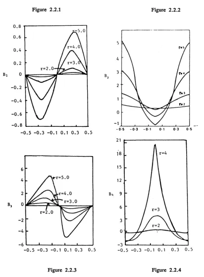
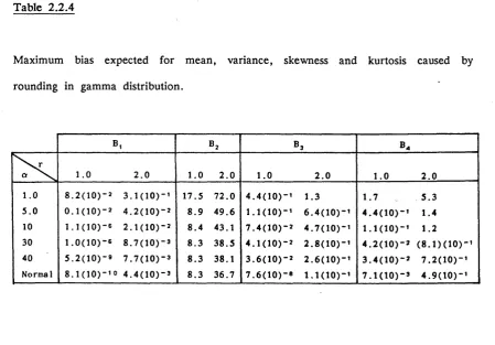
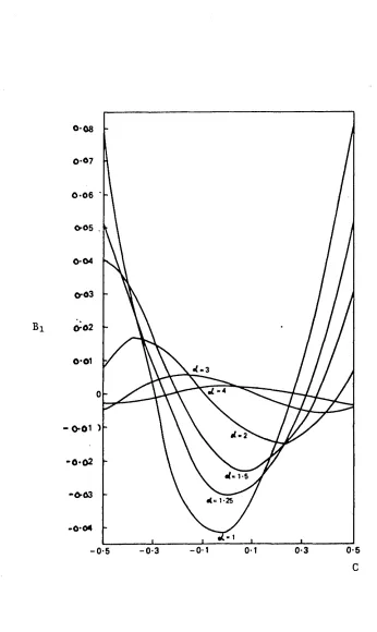
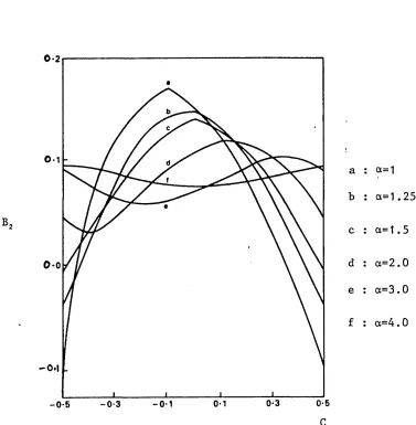
2.2.1 Characteristic function and moments of 2.4 rounded distribution

2.2.2 Moments of rounded normal and gamma 2.19 distributions

2.2.3 Relationship between the shape of a 2.36 distribution and the effect of rounding

on its moments

2.3 Bivariate Distributions 2.49

2.3.1 Characteristic function and moments of 2.50 rounded bivariate distribution

2.3.2 Bivariate normal 2.54

2.4 Conclusions 2.64

CHAPTER 3

TH E EFFECT OF ROUNDING ON TH E SIGNIFICANCE LEVEL OF CERTAIN NORMAL TEST STATISTICS

3.2 Description of the Investigation 3.5

3.3 Test Statistics 3.9

3.3.1 One sample t-test 3.10

3.3.2 Chi-squared test for variance 3.17

3.3.3 Two sample t-test 3.21

(9)

Page

3.3.5 Analysis of variance 3.36

3.4 Discussion and Conclusions 3.46

CHAPTER 4

TH E EFFECT OF ROUNDING ON THE POWER LEVEL OF CERTAIN NORMAL TEST STATISTICS

4.2 Description of Investigation 4.2

4.3.1 One sample t-test 4.5

4.3.3 Two sample t-test 4.15

4.3.4 F-test for equality of two variances 4.19

4.3.6 Compensation for rounding 4.29

4.4 Discussion and Conclusion 4.33

CHAPTER 5

TH E EFFECT OF ROUNDING ON TH E SIGNIFICANCE LEVEL AND POWER OF CERTAIN NORMAL TEST STATISTICS FOR NO N-NORM AL D ATA

5.2 Description of Investigation 5.3

5.3.1 One sample t-test 5.8

5.3.3 Two sample t-test 5.20

5.3.4 F-test for equality of two variances 5.26

5.4 Test Statistic : Exponential Data 5.36

5.5 Discussion and Conclusions 5.38

CHAPTER 6

ESTIM ATION OF ft AND a 2 FOR NORMAL ROUNDED D A TA

6.2 Maximum Likelihood Estimation 6.3

6.3 Other Methods of Estimation 6.4

6.4 Approximate EM Algorithm 6.11

(10)

Page

CHAPTER 7

ESTIM ATION OF PARAMETERS FOR ROUNDED D A TA FROM NO N-NO RM AL DISTRIBUTIONS

7.2 Gamma Distribution 7.3

7.2.1 Maximum likelihood estimation 7.4

7.2.2 Approximate maximum likelihood estimation 7.12

7.2.3 Sheppard's method 7.14

7.2.4 Naive methods 7.17

7.3 Exponential Distribution 7.19

7.3.1 Maximum likelihood estimation 7.20

7.3.2 Other methods of estimation 7.22

7.4 Discussion of Results 7.23

CHAPTER 8

CONCLUDING REMARKS 8.1-8.7

APPENDIX A

COMPUTER PROGRAMS AND OUTPUT FOR CHAPTER 2 A1

APPENDIX B

COMPUTER PROGRAMS AND OUTPUT FOR CHAPTERS B1-B16

3 AND 4

APPENDIX C

COMPUTER PROGRAMS AND OUTPUT FOR CHAPTER 5 C1-C22

(11)

CHAPTER 1

INTRO DUCTION. NO TATIO N AND REVIEW OF LITERATURE

1.1 Introduction

1.2 Rounding Process. Notation and Terminology

1.3 Literature Review

1.3.1 Relationship between the moments of the rounded variable Xr and the underlying

continuous variable X

1.3.2 Point Estimation

1.3.3 Regression

1.3.4 Tests of Significance and Confidence Intervals

(12)

1.1 Introduction

In statistics the rounding of data, ie the grouping of continuous data at the

midpoints of equi-spaced intervals, is common.

When data are collected, values are usually rounded to a common degree of

precision. This may result from limitations in the accuracy of available measuring

devices or cost restrictions necessitating the need for cheap and consequently

inaccurate methods of data collection. In other situations rounding may be

desirable to simplify subsequent statistical calculations.

As a consequence of rounding, each recorded value will have an associated error,

the size of which can have an important effect on the validity of statistical

techniques. It therefore becomes important to ensure that the advantages of

rounding are not outweighed by distortion in the information obtained.

This thesis investigates the effect on statistical techniques of the degree of precision

of the rounded data. There are four main parts in this thesis: a literature review

(Chapter 1), a discussion of the implications of rounding on the moments of a

distribution (Chapter 2), a study of the behaviour of test statistics for rounded data

(Chapters 3, 4 and 5) and a comparison of estimation procedures when the data

are rounded (Chapters 6 and 7).

1.2 The Rounding Process. Notation and Terminology

If the values of a continuous random variable X are rounded, the result is a new

discrete random variable Xr. If values of X are rounded into intervals of width

(13)

w, with midpoints Xr and the centre of the interval containing zero is cw, then

Xr has the following values.

... cw - 3w, cw - 2w, cw - w, cw, cw + w, cw + 2w, ... (1.2-1)

(1.2-1) will be known as the rounding lattice. Here c determines the position of

the rounding lattice relative to the origin (zero) and may be located anywhere

between - w/ 2 and w/2. The mathematical relationship between X and X r is such that if

cw + (n-£)w < X < cw + (n+£)w

(1.2-2)

then midpoints Xr = (c+n)w n = 0,±1,±2,...

The values of Xr will be termed the rounded data.

The following notation will be adopted throughout the thesis for the moments and

related measures.

The mth moment of the random variable X (or of the distribution of X) about the

origin and mean will be denoted by and respectively.

= E[Xm] , n n = E ^ X - ^ n

(14)

The following related measures will be used

m e a s u r e X _X

r

m e a n _M _M_r

v a r i a n c e _a 2 o- 2r

s k e w n e s s = t l

a3 «/0 l R "

M 3 ]

3

° R

k u r t o s i s _{0 2} _ V-A

° A 0 2R =

M 4 R 4 ° R

Under the 'usual' decimal rounding rule, which stipulates that data be truncated to

a certain number of decimal places (cf Eisenhart 1947) we have c = 0 . The

rounding lattice is then of the form

k j ( l O ) ^ 2 where k 1 = 0 , ± 1 , ± 2 , . . .

k 2 is a fix e d integer

However this may not always be so, as the following examples show.

0

-2 -

4

-6

-th is grouping implies

w = 2, c = £

2.5

5.5

8.5

11.5

th is grouping implies

w = 3, c = V 3

(For example: 0 - means, includes all values from zero to less than 2).

(15)

When data from a population distribution are rounded, the severity of rounding

does not depend solely on w but also on the standard deviation cr of the

population. The severity of rounding of a distribution can be regarded as the loss

of information due to the process of rounding, which is determined by the number

of points on the rounding lattice determining the distribution. If a distribution has

a small <r, it will need a smaller w to be represented by a given number of points

on the lattice, than does a distribution with a large cr. Hence the loss of

information caused by rounding is better measured by the ratio r = w/cr. This will

be called the degree of precision of the rounded data.

Estimation

Throughout the thesis the following terms will be applied to an estimator 0 of a

parameter 0.

(i) Unbiased estimator

The estimator 0 is said to be unbiased for 0 if E[0] = 0. The bias in

0 will simply be E[0] - 0.

(ii) Mean Square Error (MSE1

If 0 is an estimator of 0, then the MSE of 0 is:

(16)

(iii) Efficiency

If By, 62 are estimators of 6 based on the same sample size, then the

A A

efficiency of 0 1 relative to 6 2 is the ratio

. . MSE(0 2)

e ( B y , B 2) ---J -M S E ( 0 , )

Summary of notation used in the rounding process

w - width of the rounding interval

c - position of the rounding lattice relative to origin

r - the degree of precision of the rounded data

X - continuous random variable

Xr - a discrete random variable obtained when X is rounded into

intervals of width w, with lattice position c, and takes the value

of the interval midpoints

fjL - mean of X

/-ir - mean of Xr

cr2 - variance of X

c2r - variance of Xr

,//51 - measure of skewness of X

y/SjR - measure of skewness of Xr

/S2 - measure of kurtosis of X

/3 2R “ measure of kurtosis of X r

(17)

1.3 Literature Review

There is a large amount of literature on the grouping of data. There are many

different methods of grouping, of which rounding is one. In this literature review

the effect of rounding on statistical techniques will be reviewed. Previous work on

rounding can be broadly divided into the following areas.

1.3.1 Relationship between the moments of the rounded variable Xr and the

underlying continuous variable X

This section concerns the relationship between the moments of the unrounded and

rounded variables X and Xr respectively. Much of the past literature has

considered this relationship in terms of using Sheppard's corrections and the

justification on various types of distributions.

The early work concerning rounding concentrated on the estimation of population

moments from grouped data. Sheppard (1898) was the first to establish that for

data which had been classified into equally spaced groups, the class centre may be

used to calculate the various moments and the bias introduced by this procedure

can be connected by the use of Sheppard's corrections. Sheppard sought to find

formulae relating the moments of the grouped variables to those of the underlying

continuous data distribution. He considered the relation between the mth

population moment

.+ 0 0

(18)

of continuous random variable X with p.d.f. f(x) and the mth moment of the

grouped data:

* R i + W/ 2

f ( x ) dt XRi " W/2

where the values of X have been grouped into classes of width w and midpoints

XRi- We thus have the very familiar Sheppard's corrections:

/MR - A

» i w2

^2R — ^2 + 12

« i w2 i

^3R = ^3 4~ /*1 +00

JhnR = i= - o o

The general expression for these formulae is

B]

j- 0

where |^ j is the in te g ral part of

Sheppard based his corrections on the Euler-Maclaurin sum theorem, which

connects summation with integration. In his paper he implied that the conditions

(19)

(i) f(x) is continuous on a finite range (a,b)

(ii) f(x) is such that f(x) and the derivatives of f(x) vanish at the limits, ie

it has high order contact.

For several years after the publication of this paper the conditions under which the

corrections were valid were subject to argument. In particular, what degree of

high order contact should a distribution have before the corrections are valid?

Kendall (1938) attempted to clarify when the corrections are valid. He showed

that the conditions of the validity of Sheppard's corrections are in the main the

conditions under which the remainder term in the Euler-Maclaurin expansion used

to derive the corrections may be neglected to a satisfactory degree of

approximation. By establishing conditions under which the remainder term is small

enough to be neglected, Kendall gave the following statement concerning the

validity of Sheppard's corrections.

Let f(x) be a continuous distribution. The Sheppard's corrections (1.3-1) will be

accurate to order w^ ie to the order of the terms applied in the corrections, if

(a) the range of f(x), (a,b) is finite

(b) the order of terminal contact is k ie f(x) and its first k derivatives of

f(x) vanish at a and b

(c ) — s—— [ F ( x ) j is not large in the range ( a , b ) , wheredk+i dxK+1

F(x) = Xm

(d) 2 g ] < k.

W/2

(20)

Kendall pointed out that where the range is infinite no set of conditions as given

above can be stated. However, many such distributions taper off strongly to zero

at the ends of the range in such a way that the corrections will be valid. He

drew attention to two situations where the corrections may be inaccurate. These

are:

(i) the distribution of f(x) is markedly skewed

(ii) the degree of precision r (w/<r) is large.

Baten (1931) and Wold (1934) derived Sheppard’s corrections for the bivariate

situation. Hartley (1950) presented a simplified form of Sheppard's correction

formulae which are computationally more convenient. Also his corrections in some

cases allow for simultaneous correction for the rounding interval and shift of origin.

Expression (1.3-1) is complicated, particularly when inverted so as to express the

moments as linear functions of the rounded moments PmR- When we deal

with cumulants the relationship becomes much simpler. Under the same conditions

as for the validity of Sheppard's corrections we have

Ks - KSR - Bs s > 1 ( 1 . 3 - 2 )

where Kg and KgR are the sth cumulant of X and Xr respectively, and Bs is the

sth Bernoulli number.

The alternative result (1.3-2) was proved by Langdon and Ore (1930). Wold

(1934) provided a similar result for bivariate distributions.

(21)

Corrections to the moments where the distribution does not have terminal contact,

as in J and U shapped distributions, were first given by Pearson (1902). Pearson,

like Sheppard (1898), based his corrections on the Euler-Maclaurin theorem. Let

f(x) be a continuous distribution with finite range (a,b), where the values of x

have been grouped into classes of width w. By assuming 'that a = 0 and that the

derivatives of f(x) vanish at b, Pearson obtained the following corrections:

i i w4 wG

Mi “ MiR " 720 a 3 + 30240 &5

, W 2 W 4 w 6

M2 “ M2R “ 12 “ 120 a 2 + 30240 &4

where a,. = - [— f ( x ) l fo r s = 2 , 3 , . . . S Ldx8 " 1 J x = 0

If there is 'high contact at both ends', then as = 0, and we have the usual

Sheppard's corrections.

Using techniques similar to those of Pearson (1902), Pairman and Pearson (1918)

considered corrections to moments where there is no terminal contact at one or

both ends of the distribution. However, the corrections they developed for the

moments are often tedious to make. Sandon (1924) presented a simplified set of

formulae for where the distribution has an exponential curve. Following on the

work by Pairman and Pearson (1918), Pearse (1928) considered how the moments

should be corrected where the distribution has an infinite range. Martin (1934),

using a similar approach to that of Pearse, derived moment corrections for where

the lower range of a distribution may be unknown and as a result the width of the

(22)

Lewis (1935) suggested corrections that were more reliable than Sheppard's but not

so difficult to make as those given by Pairman, Pearson and Pearse. His approach

was to estimate the frequency curve in each interval in the rounding lattice by a

quadratic density function f(t) = a + bt + ct2. When the constants a, b and c

have been obtained for each interval, f(t) is used to determine the moments /xmR

of the rounded distribution. However his formulae for /*mR are in general long

and complex. Davies and Bruner (1943) developed a correction for the second

moment by a similar approach to that of Lewis.

The relationship between the moments of the unrounded and rounded distributions

X and Xr respectively, has mainly been obtained by the use of Sheppard's

corrections. Although these corrections are only approximate and can be unreliable

they have been regarded as the accepted method. Several authors have suggested

alternative methods to Sheppard's corrections, but none of these has come into

general use, the reaosn being that these alternative methods are generally difficult

to use and specific to certain distributions.

In communication engineering the parallel to rounding is the quantization of signals.

The theory of quantization has been developed by electrical engineers for signal

analysis. Some of the results of this theory can be adapted for use with rounded

data. However, this work has been mainly ignored in the statistical literature

concerned with rounding until Tricker (1984b) used quantization theory to derive a

relationship between the first two monents of the distribution of X and Xr. The

content of this paper forms part of the work contained in Chapter 2. A copy of

this paper can be found at the end of this thesis.

(23)

An important contribution to the theory of quantization is due to Widrow (1956,

1961), who derived the characteristic function of a quantized signal. This is

equivalent to the characteristic function of a random variable which has been

rounded according to a rounding lattice, with rounding interval of width w and

lattice position c. Using the characteristic function, Widrow obtained expressions

for the mean and variance of normal rounded data. However they are

approximate and restricted to a rounding lattice with c equal to zero. He also

considered the joint first moment of quantized signals for a bivariate normal

distribution, and gave an approximation to the bias in this moment caused by

quantization. The approximation is only suitable for c equal to zero and as shown

in Chapter 2 is incorrect.

Watts (1961) generalised the approach by Widrow (1956, 1961) to include

quantizers in which scaling (multiplying factors) and shifting (addition and

subtraction) are allowed. The probability density functions and characteristic

function of a quantized signal for univariate and bivariate distributions are derived.

Watts said little about the association between quantization and rounding. In

Chapter 2 it will be shown how the results of Watts can be adapted to consider

the effect of rounding on the moments of a distribution.

Although statistical literature concerned with rounding has made very little reference

to the work of quantization, this is not so for other subject areas. In chemistry,

Lowell (1980) extended the work of Widrow (1956, 1961) to find the first two

moments of normal rounded data for the more general case of non-zero mean.

His results could have been obtained more simply by using the work of Watts

(24)

Several authors have considered the relationship between the moments of X and

Xr for a normal population. To date, very little has appeared in the literature

concerning this relationship with respect to other populations. Holland (1975)

considered the effect of rounding on the moments of non-normal data. His

approach was as follows.

Let X be a continuous random variable with p.d.f. f(x). Values of X are rounded

to a rounding lattice with interval of width w and lattice position c. The result is

the rounded random variable Xr. Holland uses the p.d.f. of Xr given by

P [X R= c + nw)

to calculate E [Xr] and V [Xr].

c + ( n + £ ) w

f ( x ) d x , n = 0 , ± 1 , ± 2 , c + ( n - £ ) w

His approach does not provide any explicit expressions for the mean and variance

of Xr. He considered only distributions where the distribution of Xr has a closed

form or are tabulated in great detail. The two non-normal distributions considered

are the exponential and triangular. Although the possible effect of the lattice

position is ignored, Holland was the first to mention that the shape of the

distribution may be important in determining the effect of rounding on the

moments of a distribution. Elsewhere, Tricker (1984a) also derived the p.d.f. of a

rounded exponential data and investigated the distortion caused by rounding in the

mean and variance. Tricker considered the lattice effect, which he showed to be

important in determining the effect of rounding on the moments. The content of

this paper forms part of the work contained in Chapters 5 and 7. A copy of this

paper can be found at the end of this thesis.

(25)

Another paper by Tricker (1984b) uses the theory of quantization to obtain explicit

functions for the mean and variance of Xr. It examines the interactive effect of

rounding and skewness on the moments of a univariate distribution.

In Chapter 2 it will be shown how the theory of quantization can be applied to

the process of rounding. A more detailed examination of the effect of rounding

on the moments of a distribution than that given in Tricker (1984b) will be

presented.

Average Corrections

There is a distinct type of problem which also leads to Sheppard's corrections

(1.3-1) often referred to as 'average corrections'. If the rounding lattice is located

at random on the distribution, then Sheppard's corrections hold on average, no

matter what form the distribution takes. This result was first given by Abernethy

(1933). The parallel result for cumulants can be found in Cornish and Fisher

(1937). As pointed out by Kendall (1938), Sheppard's corrections regarded as

average corrections require the rounding lattice to be located at random. This

condition is not always met in practice. For example, many J and U-shaped

distributions naturally begin with an interval starting at zero. The rounding lattice

is then not located at random and Sheppard's corrections are not legitimate even

on average.

Sheppard's corrections are customarily applied to the moments about the mean of

the rounded distribution, namely by omitting the dashes in (1.3-1) and putting

P iR = = 0* ^ noted by Kendall (1938) this is legitimate for the same

(26)

for average corrections it is no longer valid to drop the dashes in order to obtain

corrections for moments about the mean of the rounded distribution.

Craig (1941) presented a set of expressions for the average correction to the

moments about the mean. If the location of the rounding lattice is random then,

for example, the average correction for the second moment is given by

<r2 = <rj - _R ₁₂+ a 2_m

where the variance of X and X r are respectively a 2 and <t 2r , and cr2m is the

variance of the means of the rounded distribution over all possible rounding lattice

positions. It is usually unrealistic to be able to obtain cr2m and in practice the

above correction has limited use.

1.3.2 Point Estimation

Maximum Likelihood Estimation

The method of obtaining a maximum likelihood estimate (M LE) from grouped data

has been extensively studied in the literature. We shall be interested in the

situation where the M L method can be applied to rounded data, ie where the

group intervals are equal and each interval is represented by its midpoint.

The M L procedure has been used by many researchers to estimate the mean and

variance of grouped normal data. Gjeddebaek (1949) presented a method of

obtaining the MLEs of /a and a 2 for a normal distribution, whether or not the

(27)

grouping is into equal intervals. However his precedure for obtaining the MLEs is

troublesome to use because of its iterative character. Gjeddebaek (1956) considered

the efficiency of the MLEs of p and a 2 from a sample of normal rounded data,

where the sample size is large. He defined the efficiency of these estimates as the

mean square error (MSE) of the MLE from unrounded data divided by the MSE

of the MLE from rounded data. He gave the asymptotic efficiencies of the MLEs

of p and <72 for various degrees of precision r. He showed that the position of the rounding lattice (c) has a negligible effect on the efficiencies of p. and o'2, if

the value of r is less than 2.0 and 1.6 respectively. Gjeddebaek (1957, 1959)

considered two types of estimator for the mean and variance of a rounded normal

distribution, these being the M L and naive estimators. The naive estimators are

the usual estimators of the mean and variance applied to the midpoints of the

rounding intervals. Gjeddebaek showed that, when Sheppard's corrections are

applied to the naive estimators, they are "practically as efficient" as the M L

estimators for r < 2.0 and n < 100.

Grundy (1952) presented a method of estimating the MLEs of p and cr2 for a

truncated normal distribution, when the data have been grouped. The MLEs are

obtained by using 'adjusted moments' and the effect of grouping on large sample

covariance matrix is discussed. When the group intervals are equal (rounding) the

iterative method for finding the MLEs is simpler than that given by Gjeddebaek

(1949). Swamy (1960) extended the work of Gjeddebaek (1949) by deriving the

MLEs of p and cr2 for rounded data from a single and doubly truncated normal

distribution. He obtained the MLEs by the same troublesome iterative method as

(28)

When parameters are estimated from rounded data, there is a probability that the

MLE will not exist. Even though this probability may tend to zero as the sample

size increases, Kulldorff (1961) referred to what are conditional M L estimators, with

the condition being existence. Kulldorff gave sufficient conditions for the existence,

uniqueness, consistency and asymptotic efficiency for M L estimators for grouped

data. However the set of sufficient conditions are complicated.

Kulldorff (1961) considered the estimation of the parameters of the normal and

exponential distributions. He found the MLEs of p and cr for rounded normal

data. He used an iterative process called the ’Scoring System' to obtain the roots

of the likelihood equations. This iterative procedure is less laborious and converges

more rapidly than the one used by Gjeddebaek (1949). When estimating p with a

known, Kulldorff showed that the optimum groups (optimum in the sense of

minimum asymptotic variance) are not very far from equidistant. However, when

estimating a with p. known the optimum groups are far from equidistant.

Kulldorff also derived the MLEs for both the scale and location parameters in the

exponential distribution, together with their asymptotic variances for rounded data.

He studied the MLE of the scale parameter. An approximation to the mean and

variance of the MLE of the scale parameter is derived by use of asymptotic

expansions. Using these approximations, he showed the extent to which the

asymptotic properties of the MLE are satisfactory. For rounded data the results

indicate that if the exponential distribution is of the form

x

F ( x |0 ) = 4 e 6 x > 0, 0 > 0

v

(29)

then the asymptotic mean and variance of the MLE of 8 can be safely used for

sample sizes in excess of 24, when r < 2.0.

Tallis and Young (1962) discussed the M L estimation of parameters for truncated

normal, log normal and bivariate normal distributions from rounded data. For

each distribution they gave only the M L equations. Algner and Goldberger (1970)

investigated the problem of estimating the scale parameter in the Pareto distribution

from grouped observations. They showed that, for rounded data, the MLE of the

scale parameter has an exact solution.

For rounded data, the MLE must usually be obtained iteratively. Since the use of

computers in statistics becomes widespread, iterative methods have been presented

for finding the MLEs. Generally the iterative techniques are for grouped data, of

which rounding is simply a special case.

Gjeddebaek (1949) used the Newton-Raphson iterative process in finding the MLEs

of p and cr from rounded normal data. Although the iterative procedure was not

very simple, he provided tables to assist with the computation. Kulldorff (1961)

described an iterative method for finding the MLEs of p and cr, when one of the

two parameters is known. He used the method of scoring, due to Fisher (1925).

This method is generally far superior to that used by Gjeddebaek (1949), in terms

of simplicity and rate of convergence. Tallis and Young (1962) also suggested the

method of scoring for finding the MLEs of p and a, since an estimate of the

variance-covariance matrix is obtained as part of the computational routine. Swan

(1969) used a Newton-Raphson procedure written in ALGOL to obtain MLEs of p

and a 2 from a normal sample which may be grouped in any way. At the same

(30)

Sidebottom (1976) gave a method and a FORTRAN program which can be derived

from Fisher's method of scoring for M L estimation of location and scale

parameters from grouped data. Wolynetz (1979a) described an algorithm and gave

a FORTRAN program which was derived from the expectation-maximisation (EM )

algorithm, for grouped and censored normal data. Wolynetz (1979b) gave an

algorithm for the normal linear model where the dependent variable is subject to

rounding. Schader and Schmid (1984) investigated the performance of the EM ,

Newton-Raphson, scoring and fixed-point methods for obtaining the MLEs of p

and a from grouped normal data. One of their main results is that the method

of scoring is best both in number of iterations and CPU time. Deken (1983) used

the EM algorithm to obtain the MLEs of grouped multivariate normal data. His

approach was to approximate the E-step in order to reduce the computer time for

the EM algorithm. However the formulae used are complicated.

Approximate Maximum Likelihood Estimation

Consider a random sample of n observations from a p.d.f. f(x 10), rounded into

intervals of width w, with midpoints yj (i= l,...,n ). If we let

■yi+w/ 2

P ( y i) = f ( x i 0 ) dx

J y i - w / 2

then the MLE of 0 is obtained by maximising

n

L ( 0 ) - n p ( y i ) ( 1 . 3 - 3 )

i= l

However, much work is often needed to obtain this, and it is reasonable to search

for an approximate method requiring less effort. Lindley (1950) established a

(31)

method for obtaining approximate MLEs for parameters of univariate distributions

under equal interval groups. His approach was as follows.

Consider a single group of width w with midpoint yj. By use of Taylor's theorem

we have

P (yi> = w f(y j) + ^ f n(y i) + 0(w 4) (1 .3 -4 )

where f(yj) and f"(yj) are the p.d.f. and second derivative respectively evaluated at

yp From (1.3-3) and (1.3-4) we have

L ( » ) - ^ [ w f ( y i ) [ l + f t + 0 (w 3 ) ]

and

lo g L ( 0 ) = ^ [ lo g w f ( y i ) + ^ 'f -C'y i) " + 0 <w3>]

If 6 0 is the MLE of 0 using the midpoints yj, then by applying the

Newton-Raphson method, using d Q as the first approximation, and adjusted

estimate is given by

6 =

e

0 +

5

where 5 = - ^-r₂₄ n

d 0 i = l

1 ^ 2[ lo s f ( y i) ]

(1 .3 -5 )

(32)

If the third derivative of f(x 10) exists the error in 5 is of order 0 (w 3), where if

the fourth derivative exists the error is of order 0 (w 4). Lindley showed that the

approximate MLEs are equivalent to Sheppard corrected moment estimators in the

case of rounded normal data. He also derived a formula for the loss in efficiency

caused by rounding.

Tallis (1967) presented a method for obtaining the approximate MLE for grouped

data. The method is a slight but convenient modification of the method of

Lindley. The modification replaces the various terms in Lindley's method by their

expectation and 5 (1.3-5) now becomes the average bias caused by grouping. He

also obtained approximate MLEs for parameters for multivariate distributions under

equal grouping and univariate distributions under unequal grouping. Tallis shows

that the approximate MLEs for rounded bivariate normal data agree with Sheppard

corrections given by Wold (1934). In Don (1981) this result of Tallis is

generalised to rounded multivariate normal data.

In the area of probit analysis Tocher (1949) obtained MLEs for grouped data. He

derived the equations for an iterative solution to the MLEs of the mean fi and

variance a 2 in the underlying normal distribution of grouped probit data. However

the steps in the iteration involve lengthy calculations and make the whole process

tedious. Using a similar approach to that of Lindley (1950) he obtained

approximate MLEs for \i and a 2 where the data is rounded. These approximate

estimates are found to be equivalent to the Sheppard corrected moment estimates.

(33)

Other Methods of Estimation

Although the method of M L has been the most common approach for estimating

the parameters of a distribution for rounded data, other methods of estimation have

been suggested.

A consistent estimator for rounded data was presented by McNeil (1966). It is

computationally simpler than the MLE and is consistent even when the M LE is

not. However, it is very difficult to apply for multivariate distributions. With

today's computing facilities the computational problems in obtaining the M LE have

become less important. As a result the McNeil approach has not become a

worthwhile alternative to that of the ML.

Others who have considered alternatives to the M L approach are Yoneda and

Uchiyama (1956). They advocated the use of ordered statistics to estimate the

mean and variance of coarsely rounded normal data. The method of minimum

chi-square was suggested by Hughes (1949) to estimate the variance of rounded

bivariate normal data.

Often rounding is ignored and standard estimation procedures are applied to the

midpoints of the rounding intervals. This naive method of estimation can lead to

misleading inferences. Tricker (1984a) showed this for exponential rounded data.

He used the interval midpoints to compute the M L estimator for unrounded data.

This naive estimator has bias which does not decrease to zero as the sample size

increases. He illustrated how the magnitude of the bias is dependent on the

degree of precision of the data and on position of the rounding lattice. For

(34)

the bias in this naive M L estimator.

In past literature, estimation with regard to rounded data has concentrated on the

normal distribution. In Chapter 7 the efficiency of various estimation procedures

will be investigated when applied to non-normal rounded data.

1.3.3 Regression

Consider the regression model

Y = 1 (50 + X ^ + E (1.3-6)

where Y is the (n xl) vector of observations of the dependent variable, X is the

(nxk) matrix of the values of k independent variables, 1. is the (n x l) vector of

ones, E is the (n xl) vector of errors assumed to be uncorrelated with zero mean

and variance cr2, and = (j3t ,...,/3jc)' is the (kxl) vector of regression

coefficients to be estimated.

Durbin (1954) considered the problem of error of measurement in the variables of

the simple regression model that passes through the origin, ie /30 = 0 and k = 1

in (1.3-6). The error of measurement can be caused by several factors, of which

one can be the process of rounding. Durbin devoted part of his paper to the

effect of rounding on the least squares estimate (LSE) of /3r He stated that,

under the traditional assumptions concerning errors of measurement, the LSE of /3,

will be unbiased for rounded data. However, as pointed out by Haitovsky (1973,

Ch 6), one of the assumptions concerning errors of measurement is that the errors

are uncorrelated with the correct values. He showed that, for rounded data, this

(35)

is not so and that Durbin's statement about the bias in LSE of /31 is in doubt.

Haitovsky (1973) considered the rounding in the simple regression model (k = 1 in

1.3-6). He investigated the bias in the LSEs of 0 Q and 01 for rounded data that

takes into account the correlation between the rounding error and the correct

value. He derived approximate formulae for the bias in the LSEs of 0 Q and 01

when Y and X are both subject to rounding. He showed that if the distributions

of the independent and dependent variable are symmetrical and unimodal then:

(i) the direction in the bias in the LSEs depends on whether the number

of categories into which the independent variable is grouped is larger or

smaller than the number of categories into which the dependent variable

is grouped

(ii) the bias and loss in efficiency in the LSEs is minimized when the

independent and dependent variables are grouped into the same number

of categories.

Swindel and Bower (1972) considered the regression model (1.3-6) where the

independent variables are subject to rounding. They showed rounding will cause

the LSEs of the regression coefficients to be biased, and derived bounds on this

bias. However these bounds are dependent on knowing the true value of the

regression coefficients and the rounding errors.

Beaton, Rubin and Barone (1976) investigated the effect of rounded data on the

regression model (1.3-6). They use computer simulation to recreate the unknown

(X,Y) by adding a uniform rounding error onto the rounded value (Xr.Xr)- This

(36)

each time. The main point of this method is that these recreated LSEs are useful

in showing the possible disturbances due to rounding. Beaton et al (1976)

illustrated their technique on the much analysed Longley (1967) data. They

showed how high correlation between the independent variables should be avoided,

in order to reduce the effect of rounding. A simple adjustment strategy for

improving the LSE of 0 is given when the data is rounded. They suggested that,

for small rounding intervals an improved LSE of 0 can be obtained by adding

w 2/1 2 to the diagonals of the sample covariance of (Xr.Yr).

Beaton et al (1976) assumed that the rounding error is independent of the rounded

value and uniformly distributed with mean zero and variance w 2/12. In fact the

rounding error is conditional on the value of the rounded observation and

knowledge of the rounded value can convey information about the rounding error.

Dempster and Rubin (1982) pointed out the failure of Beaton et al to use a

conditional distribution for the rounding error. They illustrate by using an artificial

example how the adjustment suggested in their paper to compensate for rounding

error can lead to increased bias in the LSESs. For model (1.3-6) Dempster and

Rubin considered three sample approaches to the problem of rounding in (X ,Y ) for

least squares regression, these being:

(i) ignore the effect of rounding on the data

(ii) add an adjustment of w 2/12 to the diagonals of the covariance

matrix (Beaton et al; adjustment)

(iii) subtract an adjustment of w 2/12 from the diagonals of the

covariance matrix (Sheppard's correction).

(37)

Approaches (i) and (ii) are shown to lead to considerable bias in the regression

coefficients, especially when the design matrix is ill-conditioned.

Likelihood analysis, which uses the conditional distribution of the unrounded values

given the rounded value, can produce a more reliable adjustment. When the

width of the rounding interval is small, this adjustment is shown to be (iii) above

in two situations

(a) (X,Y) is jointly normal

(b) normal residuals, large sample and the distribution of the independent

variables are 'regular' (meaning the distribution is relatively smooth).

An adjustment (iii) is suitable only for small rounding intervals. For 'moderate'

rounding the adjustment required will vary considerably depending on the

distributional form of the independent variables.

Cameron (1987) investigated the effect of rounding on parameter estimation in

simple regression, where the error has different distributional forms. He compared

two methods of estimating the parameters. In the first, the rounding is ignored

and the LS estimators are applied to the midpoints of the rounding intervals; this

method is referred to as the OLS method. The second is the M L method for

grouped data, which recognize the rounding in the data. A simulation experiment

demonstrated that, where the errors are normally distributed, the OLS method

yields virtually identical point estimators of the intercept and slope compared to

those obtained from the grouped M L method, when the degree of precision r is

less than one. While for the same range of r, the OLS method gives only slightly

(38)

deviates from the normal curve, the OLS method does not necessarily perform

well. As the skewness in the errors increases, so does the distortion in the

parameters when the OLS method is used.

The use of the M L estimators for regression models, for grouped data has lead to

some research into iterative procedures. Burridge (1981) determined for a class of

regression models (eg normal, logistic, extreme value), where the dependent

variable is grouped, a parameterization in which the log-likelihood is guaranteed to

be concave, thereby ensuring the existence of a global maximum. He

demonstrated by simulation that this reparameterization of the regression model

improved considerably the speed of convergence of iterative procedures based on

the Newton-Raphson method.

Burridge (1982) presented a more general set of results on concavity of

log-likelihoods, derived from grouped data. In general, concavity of the

log-likelihood alone does not imply that the MLE exists. In Burridge (1986), for

regression models considered in Burridge (1981), a necessary and sufficient

condition is given for the existence of MLEs, where data is grouped.

Approximate Maximum Likelihood Estimation in Regression Models

The method of obtaining MLEs of the parameters in a regression model, where the

likelihood recognizes the rounded data is often said to produce the "full maximum

likelihood" (FM L) estimates. As finding these usually calls for considerable

computational effort, alternative methods have been used.

(39)

Fryer and Pethybridge (1972) extended the approach of Lindley (1950) to obtain

approximate MLEs for the parameters in the simple regression model (k = 1 in

1.3-6), when (X,Y) has a bivariate normal. They considered having either or both

of the variables rounded. Their simulation results suggest that the approximate

MLEs and their corresponding variances are adequate substitutes for the FM L

estimates if the degree of precision r does not exceed 1.6.

Pethybridge (1973) extended the work of Fryer and Pethybridge (1972) to

polynomial regression. In Pethybridge (1975) the approximate MLEs in the simple

regression model for rounded data are considered from two aspects: firstly their

behaviour in small samples, secondly, if slight departures from normality of X have

any effect on their suitability in large samples. Simulation results suggest that the

approximate MLEs and their corresponding variances are suitable substitutes for the

FM L estimates if r does not exceed 0.8 when the sample size is 25, and if r does

not exceed 1.6 for sample sizes of at least 100. Also slight 'non-detectable'

departures from normality in X are shown not to affect the acceptance of the

approximate MLEs as a suitable approximation to the exact MLEs when the sample

size is large.

Indrayan and Rustagi (1979) considered the regression model (1.3-6) where the

independent variable Y is subject to rounding and the errors are normally

distributed. They derived approximate MLEs for the parameters in the regression

model. Simulation experiments showed how these approximate MLEs compare with

those based on unrounded data. However, the authors provided no indication of

the value of r that will give a suitable agreement between the approximate MLEs

(40)

1.3.4 Tests of Significance and Confidence Intervals

In the literature the effect of rounding on tests of significance and confidence

intervals has been generally unexplored. For example, how will the distribution of

a test statistic be altered by rounded data and which statistical tests are sensitive to

rounding? Answers to such questions as these have not been well covered in the

literature.

William Sealy Gosset, better known as "Student", was probably the first to discuss

the effect of rounding on statistical procedures. In his paper on "The probable

error of the mean", Student (1908) discussed the statistical effects of using "wide

groups" for data. Student's experimental results suggest that the distribution of the

one sample t statistic for rounded and unrounded data will be approximately the

same if the sample size is large.

A classic statistical procedure for rounded data is the use of Sheppard's corrections.

However, Fisher (1936, Ch 3, App D ) advised that

These adjustments should be used for purposes of estimation, but not usually

for tests of significance.

This was reiterated by Eisenhart (1947, p203), who pointed out that use of

Sheppard's correction can make the t value imaginary as the corrected estimate of

variance can be negative. Further reiteration came from Gjeddebaek (1968). He

showed that S 2p/n is a better estimate of the sampling variance of Xr, than the

corrected alternative (S2p -w 2/12)/n; where Xr and S 2r are the usual estimates of

the population mean and variance, applied to rounded data. His advice is that

(41)

S2r should be used without Sheppard's correction when XR and S 2R are

brought together in testing procedure or in a statment of confidence limits for

the population mean.

Krutchoff (1967) pointed out that rounding can cause the F statistic for equality of

two variances to have a non-zero probability of a zero in the demoninator. Thus

the mean of this statistic will not exist.

Eisenhart (1947) was the first to study in any detail how rounding affects a test

statistic. For samples drawn from a rounded normal population, he concluded:

If the sample size n is sufficiently large and the rounding interval width w is

sufficiently small to render the discontinuities in the rounded distribution

negligible then the distribution of the

(i) test statistic

X> - <n-l>S g/[«r* + £ ] .

will closely approximate a x 2 distribution with n-1 degrees of freedom

for rounded data

(ii) test statistic

= (Xr-fO

SR/y n

will closely approximate a t distribution with n-1 degrees of freedom for

rounded data.

(42)

given value of n, before (i) and (ii) may be considered correct. His criterion for

judging the suitability of a particular coarseness of rounding was based on the

probability of the sample variance, S 2r for the rounded data being zero. He

proposed that P[S2r = 0|n,w ] < 0.001 evaluated on the assumption that sampling

is from a normal population be adopted as a definition of values of n and w for

which (i) and (ii) can be safely used on rounded data. Eisenhart recommended

the following combinations of n and r (w/(r) for which the test statistic \ 2 an<2 *

can be used to make inferences about <r2 and /i respectively.

Degree of Precision r______________Sample size

r < 0.005 n > 2

r < 0.01 n > 3

r < 0.5 n > 5

r < 0.8 n > 6

r < 1.0 n > 7

Eisenhart also suggested that, if the values of (n,r) satisfy the recommendation

given above, then the F-test for equality of two variances may be applied to

rounded data.

The problem with Eisenhart's recommendations is that they are based on the

probability of the sample variance from rounded data being zero. This gives no

indication of the performance of the test statistic with respect to level of

significance or power under rounding. In Chapters 3 and 4 this issue is

investigated.

(43)

Preece (1982) examined text book examples of the paired t-test with respect to the

degree of precision of the recorded data. He illustrated how the paired t statistic

depends crucially both on the rounding interval and position of the rounding grid

relative to the origin. Using a similar approach to that of Preece, Riley, Bekele

and Shrewsbury (1983) investigated the effect of rounding on the analysis of

variance. The degree of precision of data sets taken from standard literature was

varied, to illustrate how rounding effects the main squares. Their analysis showed

that data could be rounded appreciably before loss of information became

signficiant.

The investigations by Preece and Riley et al consisted of looking at the effect of

rounding on specific examples. As a result no general conclusions could be

established about the performance of a test statistic for rounded data.

1.3.5 Rules of Rounding

Throughout the literature various rules have been suggested for the degree of

precision that should be used when recording data. The rules are mainly

concerned with data rounded from a normal distribution. There seems to be no

standard rule. The purpose of this section is to summarise the rounding rules that

have been adopted in the literature.

Although Student (1908) discussed the statistical effect of using poor precision in

recording data, it was Fisher (1922) who was probably the first to suggest a rule

for rounding data. In this paper, Fisher obtains results on the loss in efficiency

due to grouping when the parameters of a normal distribution are estimated from a