Trust and Reciprocity in 2-node and
3-node Networks
Alessandra Cassar, ac and Mary Rigdon, mr
University of San Francisco, University of Michigan
26 January 2008
Online at
https://mpra.ub.uni-muenchen.de/7005/
Trust and Reciprocity in 2-node and 3-node Networks
Alessandra Cassar
University of San Francisco
Mary Rigdon
University of Michigan
∗January 26, 2008
Abstract
In this paper we focus on the interaction between exogenous network structure and bargaining
behavior in a laboratory experiment. Our main question is how competition and cooperation
in-teract in bargaining environments based on networked versions of the investment game. We focus
on 3-node networked markets and vary the network structure to model competitionupstream—
multiple sellers paired with a monopsonistic buyer—and competitiondownstream—a monopolistic
seller paired with multiple buyers. We describe two kinds of models of trust for such networked
environments, absolute and relativized models, and use this structure to generate a general
hy-pothesis about these environments: that information crowds in cooperation on the competitive
side of the market. The experimental results support this hypothesis.
1
Introduction
It is well-known that bilateral bargaining under incomplete contracts is often cooperative and efficient
even in environments where the equilibrium path favors no exchange at all. A buyer and seller manage
to trade, often sharing the gains from exchange. But many environments have more structure to them
than is represented by bilateral exchange: a principal may invest simlutaneously in multiple agents,
and an agent may represent the interests of more than one principal. In each case, all of the connected
parties are actors in the transaction and the structure of the network they find themselves in may
have consequences for their choice behavior in the (thin) market in which they operate. The strategic
behavior of real agents is thus often embedded in social networks, and so there is a need to study that
behavior as it occurs as part of a complex system in which agents are linked to each other (Granovetter,
1985; Barabasi,2002;Raub and Wessie, 1990).
There is a large literature, both theoretical and experimental, that focuses on strategic behavior in
networks. The scope of issues is broad: the amount of cooperation and coordination achieved in various
networked markets (Cassar, 2007; Cassar and Wydick, 2008); borrowing behavior in informal credit
arrangements (Mobius and Szeidl, 2007); different patterns of contagion in financial crises (Cassar,
2001;Eisenberg,1995;Allen and Gale,2000); ultimatum bargaining outcomes (Corominas-Bosch,2004;
Fischbacher,et al.,2003); employment and inequality in labor markets (Calvo-Armengol and Jackson,
2004); institutional efficiency (Deck and Johnson, 2004); social capital (Karlan, et al., 2005); social
learning (Gale and Kariv,2003); provision of trust when contract enforcement is weak or nonexistent,
and transmission of information about profitable trade opportunities (Rauch and Casella,2001;Cassar,
et al.,2004).
In this paper we focus on the interaction between exogenous network structure and strategic
be-havior in a bargaining environment. Similar to some other research, our focus is on off-equilibrium
but efficient cooperation. Unlike previous research, however, we focus on situations in which there are
gains from the exchange between parties and in which equilibrium favors no exchange.
There are two ways that bargaining may be implemented on a network. The first,bargaining over a network, is familiar from the evolutionary game theory literature. Here individual interactions remain bilateral, but there is imposed structure on the population from which partners are drawn. Thus,
agents on a ring bargain with their neighbor to their left and to their right, and agents on a lattice
might bargain with the local Moore (8) neighbors or their von Neumann (4) neighbors. In each case,
the individual interactions remain bilateral, but the population forces the pairing to be non-random,
and this (in the context of an updating rule like the replicator dynamics) can drive the population
toward efficient outcomes (Skyrms,2004;Axelrod,et al.,2002;Blume,1995;Ellison,1993;Nowak and
May,1993;Skyrms,2004;Samuelson,et al.,1998).
The other way of implementing bargaining on a network, what we callnetworked bargaining, changes the topology of the bargaining environment itself to model structured interactions for more than two
agents. Here the interactions are no longer bilateral, and the network structure is part of the strategic
environment. We focus on this type of interaction between network and bargaining, and in particular
Our main question is how competition and cooperation interact in bargaining environments based
on networked versions of the investment game. The level of competition in a market is likely to be
a function of several things: the network structure the agents find themselves in, the information
available to the parties in the exchange, and the agents likelihood of meeting exchange parties again.
Thus, competition is a function, in part, of who the agents are (e.g., how thin the market is), their
roles (e.g., buyer or seller), and also what each agent knows about the behavior of the other parties
to the interaction. We focus on 3-node networked markets and vary the network structure to model
competitionupstream—multiple sellers paired with a monopsonistic buyer—and competition down-stream—a monopolistic seller paired with multiple buyers. We use this structure to generate a general hypothesis about these environments: that information crowds in cooperation on the long-side of the
market. Our experimental results generally support this hypothesis.
The next section characterizes two networked versions of the investment game. Section3describes
the difference between absolute and relativized trust and develops a model of trust in the standard
investment game using framework fromCox, Friedman, and Sadiraj(in press) and extends the model
then to the networked game. Section4discusses two kinds of information flow in the network, partial
and full information, and puts forward our main hypothesis about the relationship between information
flow in the network and rates of cooperation among the agents. Section5discusses the experimental
design and implementation and Section6 contains the results. The final section concludes.
2
2-node and 3-node Networked Investment Games
The standard bilateral investment game is the limiting case of networked bargaining: it is a 2-node
(dyadic) bargaining network, with one node occupied by Sender and the other by Receiver. Sender
(S) is paired with Receiver (R), and each are endowed withM. In the first stage,S sends an amount
X (0 ≤X ≤ M) to R. That investment grows by some factor r > 1. In the second stage, R can
return some amountY ofrX to S. The final payoff to S is M−X+Y and the final payoff to Ris
M+rX−Y.
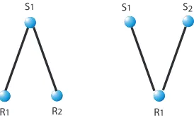
We use the 2-node case as a point of comparison, but focus on 3-node (triadic) networked investment
games. In the networks we consider, each of the nodes is a different player—either a Sender or a
Receiver—and the network is created through the interaction of the players. Moreover, we focus on
S1
R1 R2 R1
[image:5.612.237.374.85.170.2]S1 S2
Figure 1: Triadic Networks
is on the Receiver’s side (i.e., the buyer’s) of the market; in the other the induced competition is on
the Sender’s side (i.e., the seller’s).
The first triadic network structure adds an additional Receiver so that the Sender is paired with
two Receivers,AandB (see Figure1, left); we call this network structure [1s-2r]. S begins withM,
andRA and RB each begin with M. In the first stage, S chooses an amount XA of his endowment
(0≤XA≤M) to send toRAand an amountXB(0≤XB≤M) to send toRB, whereXA+XB≤M.
The investedXAandXBare then multiplied by a growth factor,r >1. In the second stage,RAchooses
some amountYA of rXA, and RB some amount YB of rXB, to return to Sender. In this structure
Sender is a monopolist and there is downstream competition between ReceiversAandB.
The other triad reverses the asymmetry between Senders and Receivers: two Sendersαandβ are
paired with one Receiver (see Figure1, right); we call this network structure [2s-1r]. SαandSβ each
begin withM, andR begins withM. In the first stage,Sαchooses an amountXα (0≤Xα≤M) to
send toR, and similarlySβ chooses an amountXβ(0≤Xβ≤M). The investedXαandXβ are then
multiplied by a growth factor,r >1. In the second stage,R then chooses some amountYαofrXαto
return toSαand some amountYβ ofrXβ toSβ.1 In this structure Receiver is a monopolist and there
is upstream competition between Sendersαandβ.
The subgame-perfect equilibrium in the dyadic investment game hasSopting out, investing nothing
and all players earn only their initial endowments ofM. Extending the standard backward induction
argument to the triads: independent of whether the market power is concentrated in the hands of
the Sender (downstream competition) or the Receiver (upstream competition), assuming that agents
are Bayesian maximizers, Receivers will keep any investment. Under the standard common
knowl-edge assumptions, Senders know this and (preferring more to less) invest nothing. Since the relevant
1Note that Rreturn choices are bounded by the investment made by a particular sender, not by the aggregate
inequalities between utilities are strict, the equilibrium is unique. Thus the equilibrium path in the
triads also favors no exchange between Senders and Receivers.
3
Modeling Trust: Absolute and Relativized Trust
What distribution or outcome an agent prefers might depend not only on what the options for
dis-tributing the goods are when she makes her choice, but on how she arrived at that set of options.
If preferences are understood purely classically, of course, this is problematic. But in the case of
bargaining environments, there is ample experimental evidence of exactly this kind of dynamics of
preferences. There are two relevant results. First, cooperative outcomes are chosen by second movers
in investment and trust games at different rates (across subjects) depending on different histories of
the game leading up to an information set (see, e.g.,Croson and Buchan,1999;Ortmann,et al.,2000;
Glaeser,et al.,2000;Fehr,et al.,2002;McCabe,et al.,2002;Engle-Warnick and Slonim,2005;Rigdon,
2007). With an interesting caveat, rates of return increase as a function of investment.2 Second, if
that history involves an opportunity cost for first movers (i.e., the difference between first movers’
outside option and the payoff received if the second mover chooses defection is strictly positive), so
that the cooperative move by a second mover can be deemed “reciprocal”, there is comparably more
cooperative play by second movers than if there is no such opportunity cost (McCabe,et al.,2003).
Thus there is empirical support for the hypothesis that a Receiver in these environments chooses
cooperatively only when Sender’s action carries a signal of trust. Therefore by giving a more
pre-cise characterization of when a Sender action carries a signal of trust, we can generate more prepre-cise
predictions for the conditions under which Receivers reciprocate, and test those predictions in the
laboratory.
Trust in bilateral bargaining games like the investment game is, in general, measured by how much
Sender invests. Given the empricial hypothesis that Receivers respond differentially to different levels
of trust, it is then straightforward that what counts as trusting behavior (according to Receivers) is
the investment level. But once we have non-trivial networked bargaining, there are multiplie measures
that might be at work. In [1s-2r] the question istrust in whom? Does trust in Receiver A just equal the amount sent to A,XA (anabsolute measure), or does it also depend on the amount sent to the other Receiver,XB (arelativized measure)? In [2s-1r] the question istrust from whom? Does trust
2The caveat is that there is a kink in returns for investment levels in the (6,8) interval in the standard baseline
from Senderαjust equal the amount sent fromα(absolute),Xα, or does it also depend on the amount
sent from the other Sender,Xβ (relativized)?
Our main concern is to examine whether and how changing the topology of investment games
by imposing network structure on them can crowd-in efficient, off-equilibrium path play. Our initial
hypothesis, to be refined below, is that it does. Our conjecture is crowding-in is due to two interacting
factors: (1) what counts as a signal of trust in these networked games is some relativized trust measure;
and (2) if the information conditions are right, that can get exploited to drive choice behavior toward
more efficient play. Thus, for our purposes, it is not important to look to any one particular model of
relativized trust. Rather, we can assume thatany reasonable model of relativized trust says that it is some increasing function of differences in amount sent, and then test the class of all such models all at
once. It is still useful to see some simple models of relativized trust, and so we provide some examples.
3.1
Trust in 2-node Networks
In the standard 2-node investment game, the distinction between absolute and relativized trust
col-lapses: the amount sent by Sender (X) is considered a signal of trust. Intuitively, this is because as the
investmentX gets larger, so does the pie of gains from exchange that Receiver has to divide between
them. So Receiver’s space of options gets bigger and better while Sender’s best-case options get bigger
and better but also herworst-case option is worse than had she not sent anything at all.
To turn this intuition into a more precise characterization, we need to describe how agents’
prefer-ences can be conditional on the opportunities they face. The idea of “dynamic preferprefer-ences”—that an
agent’s preferences over bundles might depend on how she arrives at the choice between bundles—is, of
course, not new (see e.g. Sen(1997)). What is new is to use such a characterization of when an action
carries a signal of trust to derive predictions for off-equilibrium cooperative behavior by Receivers
in bargaining environments. Our characterization of trust in 2-node investment games uses some of
the framework from a non-parametric model of preferences byCox, Friedman, and Sadiraj(in press).
But we depart from and extend the framework considerably to better suit our purposes, providing an
interesting set of hypotheses for network environments.3
3The main point of departure is that our concerns are different: we want a framework for characterizing a set of
Begin with ann-player extensive form game. The basic idea is that agents can have very different
preferences depending on what the set of feasible options is. Thus we conditon preferences on such
sets. For a given game, let Π be the total set of possible payoff distributions. We will generally assume
that this is a compact, convex subset ofℜ2
+. Since our interest is in 2-node and 3-node investment
games, three types of distributions will be particularly relevant (where wis Sender’s payoff and z is
Receiver’s payoff, and similarly forzA/B andwα/β):
• 2-node (baseline): π= (w, z)
• 3-node [1s-2r]: π= (w, zA, zB)
• 3-node [2s-1r]: π= (wα, wβ, z)
Anopportunity set F is a non-empty subset of Π. Opportunity sets are thus just feasible budget sets. Rather than preferencessimpliciter, we want to talk about an agent’spreferences given an oppor-tunity set. Given an opportunity setF,i’s preferences givenF is a well-defined ordering overF that is convex and continuous. What we care about is that playeri’s preferences givenF can be represented
by a smooth utility function ui(·|F) such that ∂u∂πi(·|iF) > 0. Two possibilities are noteworthy here.
First, it is possible thati (given F) cares about j’s payoff: ∂ui(·|F)
∂πj >0. Second, it is possible that
ui(π|F) 6= ui(π|F′) even when F ⊆ F′ . That is because the shape of i’s preferences may well be
affected by the set of opportunities she faces. It is convenient to identify what, given an opportunity
setF, a maximizing agent i’s best outcome is ifiis an own-payoff maximizer; here we abuse notation
(slightly, and to no harm) and writeπ∗(i|F). This is the maximum feasible payoff to iin opportunity
setF.
In the 2-node investment game, then, it is straightforward to say when one of Sender’s actions is
more trusting than another: just in case it determines a better budget space for Receiver and how
much better is not dwarfed by how much better it is for Sender. That is:
Definition 1.
1. Opportunity setGis at least as generous asF,GDF, iff:
a) π∗(R|G)≥π∗(R|F); and
b) π∗(R|G)−π∗(R|F)≥π∗(S|G)−π∗(S|F)
X carries at least as strong a signal of trust as X′ if the opportunity set determined byX is at least
as generous as the opportunity set generated byX′.
Thus, to say that one action carries a stronger signal of trust than another is to say that the first
generates an opportunity set Gthat is more generous than the opportunity set F generated by the
second. To say thatGis more generous than F is just to say that a maximizing Receiver can do no
worse inGthan inF and thathow much better Rcan do inGas compared toFisn’t trumped by how much better Sender can do inGas compared toF. This second clause, notice, would not be satisfied
if Sender faced no opportunity cost to investing.
Since opportunity sets are determined by Sender’s action, it is sometimes useful to write them as
a function of that action. In the investment game, Sender’s choice is an investment bundle. In the
2-node case, it is a value forX; in the [1s-2r] case, it is a pair (XA, XB); and in the [2s-1r] case, each
Sender makes an investment choice,Xαand Xβ, and each thereby determines an opportunity set for
the Receiver. Wherecis an investment choice by a Sender, let Ω(c) be the opportunity set this choice
determines.
Example. Consider two possible actions, or investment choices, by Sender in the 2-node investment
game with endowmentM = 10 for each player and a growth rater= 3 (standard parameter values
used in the investment game): X = 2 andX′= 8. Intuitively, the second action represents a stronger
signal of trust than the first. This is confirmed by the model since Ω(X′ = 8)✄Ω(X = 2). To
see this, let F = Ω(X = 2) and G = Ω(X′ = 8). Then note that, for any chosen value for X,
π∗(R|Ω(X)) = 3X+M. Thus, π∗(R|G) = 34> π∗(R|F) = 16. Hence a maximizing Receiver does
better in G than in F. Second, note that π∗(S|Ω(X)) = M −X+ 3X—that is, the highest profit
for Sender, given some initial choice for X, is to get all of the gains from exchange back. Now,
π∗(S|G)−π∗(S|F) = 26−14 = 12, which is smaller than π∗(R|G)−π∗(R|F) = 18. Hence the size
of the potential windfall to Receiver for being inG is greater than the potential windfall to Sender.
Therefore,G✄F.
3.2
Short-side Trust: [1s-2r]
We now turn to 3-node networks in which the distinction between absolute and relativized models does
not collapse. First, consider the case of [1s-2r]. Sender chooses an investment bundle (XA, XB) such
investments is viewed by both ReceiverAand how that same bundle is viewed by ReceiverB. Since a
single bundle could be quite trusting to one receiver and not to another, we have to measure trust-in-A
(trustA) and trust-in-B (trustB).
An absolute model of trust says that ReceiveriviewsXias a signal of trust, full-stop. Thus trusti
depends on comparingRi’s opportunities toS’s, but only those ofS’s that are “local” to interaction
withRi. If this is the case, thenX−i does not matter. Such a model would predict nono downstream competition. We instead develop a relativized model: trusti depends on comparingRi’s opportunities toS’s “global” opportunities. Thus, since S’s global opportunities depend in part on the link shared
withR−i, X−i matters to the level of trusti signalled by the investment bundle. Such a model will
predictdownstream competition between the two Receivers.
Since trust levels are tied to opportunity sets, there is no fact of the matter as to whether one
opportunity set is “more generous than another” simpliciter in a 3-node network. So we generalize Definition1, relativizing to a particular receiver. We do this in a way that links RA’s opportunities
andXB (and vice versa), thus making this a relativized model of trust.
Definition 2.
1. Opportunity setGis at least as generous to Receiverias F, GDiF, iff:
a) π∗(Ri|G)≥π∗(Ri|F); and
b) π∗(Ri|G)−π∗(Ri|F)≥π∗(S|G)−π∗(S|F)
2. Gis more generous thanF,G✄iF, iffGDiF andF 4iG
Let Gi be Ri’s opportunity set determined by investment bundle X = (XA, XB) and Fi be Ri’s
opportunity set determined byX′= (X′
A, XB′ ). X carries at least as strong a signal of trusti asX′ if the opportunity set determined byX is at least as generous as the opportunity set generated byX′.
So far, this looks like a mere notational variant of the earlier definition: we have swapped Ri for
R. But, as we will see below, this is not really true. That is because the term involving Sender in
Condition (b) depends on Receiver −i’s behavior when faced with opportunity sets G−i and F−i.
Thus while it is true that payoffs to the receivers are independent (neither a function of the other),
whether an opportunity set is more generous than another toRi depends on the behavior (and so on
The following observation characterizes how differentially a bundle has to favor a Receiver in [
1s-2r]—say, ReceiverA—for that bundle to constitute a signal of trustA.
Observation 1. Consider two (potential) investment choices by Sender, and letG= Ω(XA, XB) and
F = Ω(X′
A, XB′ ). Then G✄AF only if the difference in investments in A are at least (r−1)-fold greater than those inB.
Proof. By definition,GDAF only if:
Condition (b) π∗(A|G)−π∗(A|F)≥π∗(S|G)−π∗(S|F)
The structure of the investment game gives us the following identities forRA’s payoffs (whereris the
rate of growth):
π∗(A|G) =M+rXA
π∗(A|F) =M+rXA′
(1)
Similarly for Sender’s payoffs:
π∗(S|G) =M −XA−XB+rXA+rXB
π∗(S|F) =M −XA′ −XB′ +rXA′ +rXB′
(2)
The LHS of Conditon (b) can be simplified a bit:
M +rXA−M +rXA′ =r(XA−XA′) (3)
Similarly the RHS:
= (M −XA−XB+rXA+rXB)−(M−XA′ −XB′ +rXA′ +rXB′ ) (4)
can be simplified to:
(r−1)(XA−XA′) + (r−1)(XB−XB′ ) (5)
So the requirement imposed by Condition (b) is that:
r(XA−XA′ )≥(r−1)(XA−XA′ ) + (r−1)(XB−XB′ ) (6)
And that is equivalent to
Which finally yields:
XA−(r−1)XB≥XA′ −(r−1)XB′ (8)
Somewhat surprisingly, the comparative level of trustAbetween two investment bundlesX andX′
requires a corresponding difference in investment level to B across those bundles. Notice that this
states a necessary, and not a sufficient, condition on relative trust. Thus, the strength of signal of
trust inAcarried by a bundleX is in part a function ofXA−XB, which is what we care about.
3.3
Long-side Trust: [2s-1r]
Next, consider the case of [2s-1r]. Here an investment bundle (Xα, Xβ) in Receiver is determined by
the joint actions of Senderαand Senderβ. The question is how the bundle of investments is viewed
by Receiver. Since there are two independent parts of that bundle (one from Senderαand one from
Senderβ), part of that bundle could be quite trusting and the other part not trusting. So we have to
measure trust-from-α(trustα) and trust-from-β (trustβ).
An absolute model of trust says that Receiver viewsXi as a signal of trusti. Thus trusti depends
on comparingSi’s opportunities toR’s, but only those ofR’s that are “local” to interaction withSi.
If this is the case, then X−i does not matter. Such a model would predictno upstream competition. We again develop a relativized model: trusti depends on comparingSi’s opportunities toR’s “global”
opportunities. Thus, sinceR’s global opportunities depend in part on the link shared with S−i, X−i
matters to the level of trusti signalled by the investment bundle. Such a model will predictupstream competition between the two Senders.
It is sufficient to say when investment bundles signal trustα and trustβ. In the [1s-2r] network,
what is relevant is how different investment bundles are viewed by Receivers, each from their own
point of view. In [2s-1r], however, what is relevant is how a single investment bundle affects what the
Receiver thinks about the two independent Senders: given the generosity of the space of opportunities
Rfaces, we want to modelα’s contribution to that andβ’s contribution to that.
Given an investment bundleX = (Xα, Xβ) that determines an opportunity setG(note that this is
a set of triples, as in the [1s-2r] network) we will give a comparative assessment of whenG’s relative
generosity is due toSα as opposed to Sβ. There are different ways of modeling this; we focus on a
Notice that we can restrictGby eliminating one of its coordinates—say the coordinate for Sender
α’s profits; such a restriction is the α-free slice of G. Thus theα-free slice ofGis the set of possible distributions inGto Receiver and Sender β. This allows us to evaluate relative generosity of G, an
opportunity set that is a function in part ofα’s investment, while ignoringα’s potential profits inG.
Similarly, we can also take the β-free slice of G: the possible distributions inG involving Receiver and Sender α. Since G is a set of ordered triples, these slices are planes (sets of pairs) and are
like opportunity sets from the 2-node investment game, except that Receiver’s profits reflect that he
is linked with two Senders. But they are (2-person) opportunity sets, and so can be compared for
relative generosity. Receiver’s range of profits are the same in these two slices, and so his maximum
profit is the same. Thus if the slices differ in their generosity, it must be because one of the Sender’s
has a higher maximum profit in his slice than the other has in his; the former is less generous.
Definition 3. LetGbe the opportunity set determined by investment bundleX= (Xα, Xβ).
1. Restricted opportunity sets:
a) α-free slice of G: G\α={(wβ, z) : (v, wβ, z)∈Gfor somev}
b) β-free slice ofG: G\β={(wα, z) : (wα, v, z)∈Gfor somev}
2. Senderiis at least as generous inGas Sender j is iffG\iDG\j
The level of trusti signalled by investment bundleX is at least as great as trustj iff Senderiis at least
as generous inGas Senderj is.
Observation 2. Senderi is at least as generous inGasj is iffXi−Xj ≥0
Proof. Suppose Senderiis at least as generous inGas j is. ThenG\iDG\j. But this is so iff
(a) π∗(R|G\i)≥π∗(R|G\j); and
(b) π∗(R|G\i)−π∗(R|G\j)≥π∗(j|G\i)−π∗(i|G\j)
But
π∗(R|G\i) =π∗(R|G\j) (9)
soG\iDG\j iff (b) holds. That is, iff
0≥π∗(j|G\i)−π∗(i|G\j) (10)
4
Information
We now have characterizations for relativized trust both for networks with downstream competition
([1s-2r]) and for networks with upstream competition ([2s-1r]). Given the broad empirical
general-ization that return behavior in investment games increases with signals of trust by senders, we can test
the effects of network structure on off-equilibrium but efficient behavior. But competition is a function
of more than just network structure; it is also a function of how information about the bargaining
en-vironment flows throughout that network. We look at two kinds of information flow, full and partial.4
Our main empirical hypothesis is about the relationship between the kind of information flow and the
amount of cooperation achieved among the players:
Competition for Cooperation Hypothesis (CCH) Information crowds-in cooperation on the
long-side of the market
Before turning to our experimental design and results, we will describe the CCH hypothesis in detail
in this section by describing information flows in the network and how the level of information could
be expected to impact the rates of cooperation.
Say that a network allows full information flow if: (i) every agent in the network knows every move made by every other agent at points higher in the game tree; and (ii) after the terminal nodes
are reached, there is full-disclosure about all moves. This implies that in a [1s-2r] network with full
information flow Receivers each know how much is invested in the other before deciding on a return
and both learn how the other responds through full disclosure of all moves. That is:
• RA knows the value ofXB before choosingYA
• RA learnsYB through full-disclosure
• RB knows the value ofXA before choosingYB
• RB learnsYAthrough full-disclosure
Similarly, in a [2s-1r] network with full information flow, full-disclosure implies that Senders each learn
about what the other invests following own investment choice and also learn how Receiver responds to
the other Sender’s investment:
• Sα learns the value ofXβ andYβ
• Sβ learns the value ofXα andYα
4In the standard 2-node investment game there is no room for a difference between full and partial information flow
Say that a network allows forpartial information flow if each agentonly knowsabout (i.e., has full information about) the interactions in which that agent is a trader. Note that it follows immediately
that agents on the short-side of the market know about all the interactions in that market. Moreover,
in a [1s-2r] network with partial information Receivers donot know the amount Sender invests in the other and doesnot learn how the other Receiver responds:
• RA does not knowXB
• RA does not learnYB
• RB does not knowXA
• RB does not learnYA
Similarly, in the [2s-1r] network with partial information, is one in which Senders do not learn the
amount the other invests or how the Receiver responds to that:
• Sα does not knowXβ or Yβ
• Sβ does not knowXαor Yα
Thus CCH implies that in [1s-2r], with full information flow, there is competition on the long-side of
the market between ReceiversAandB for Sender’s investment. That is because each Receiver knows
the level of trustA and trustB. So, given the broad empricial generalization about return behavior
in investment games, we would expect more cooperative return behavior by each. But in the same
network with only partial information flow, the signal of relativized trust is masked: neither Receiver
A nor ReceiverB has enough information to determine trustA and trustB.5 Thus, given the broad
empirical generalization about return behavior in investment games, we would expect less cooperative
return behavior by each.
Similarly, CCH implies that in [2s-1r], with full information flow, there is competition on the
long-side of the market between Sendersαandβ for Receiver’s attention. That is because, at the end
of each stage, each Sender knows the level of trustα and trustβ. Each also knows Receiver’s reaction
to those levels. So, if Receiver responds differentially to differences between trustα and trustβ (and
given the broad empirical generalization about return behavior in investment games, this is to be
expected), then we would expect an arms race in transfers between the Senders. But in the same
network with only partial information flow, Receiver’s differential responses to Senderαand Senderβ
cannot be traced to differences in trustα and trustβ. Thus, Receiver cannot reveal his response-type
to the long-side of the market and we would therefore expect less cooperative behavior on that side of
5Note that knowing onlyX
the market.
Note that both of these implications of the CCH depend on exploiting relativized trust measures
in the networks. We now turn to our experimental design and procedures; the results are discussed in
Section6.
5
Experimental Design and Implementation
The baseline condition is the standard 2-node investment game. We then cross type of triadic network
{[1s-2r],[2s-1r]}with type of information flow{Full Info,Partial Info}to obtain our 1 + (2×2)
conditions. All treatments reported here use repeated interactions with random-matching.6
The sessions were run at the Learning and Experimental Economics Projects of Santa Cruz
(UC-Santa Cruz) and the Robert B. Zajonc’s Laboratory (Institute for Social Research, University of
Michigan). The sessions were run May 2005 through July 2006. The only difference in the instructions
for the treatment conditions was the description of either the network structure or the information
available (see AppendicesAandBfor the [1s-2r] treatment).7
We use standard parameter values for initial endowments,M = $10, and for the growth rate,r= 3.
The experimental protocol for all treatments was single-blind. Subjects in each session were randomly
assigned roles as either Sender or Receiver.
Subjects were required to complete a quiz regarding the interaction and completed calculations of
payoffs prior to beginning, which the experimenter checked for accuracy. Subjects played a version of
the game for 40 rounds with a known end-point, being randomly re-matched with a new counterpart(s)
at the start of each round. Subjects who had previously participated in similar experiments were
excluded from recruitment. Each session had 12 subjects and took less than 1 hour to complete.
Three sessions of each treatment were conducted.
6
Results
Our experimental data support the Competition for Cooperation Hypothesis under both network
structures: information crowds-in cooperation on the long-side of the markets. The flow of information
6The complete design for this project on networked bargaining has 3 matching treatments × 2 3-node network
structures×2 information conditions; in addition to the 2-node baseline.
7Computer interface screen shots for the [1s-2r] info treatment are available at
in the environment is crucial for the competitive structure to be exploited for off-equilibrium path
cooperation.
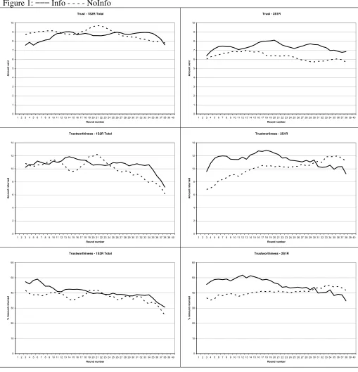
Figures 1 and 2 provide a visual display of the five-period moving averages of the results we
report below. Figure 1 displays the differences in trust and trustworthiness over time within networks
across information treatments; the dashed line corresponds to thepartial infocase and the full line
corresponds to theinfocase. Figure 2 displays the differences in trust and trustworthiness over time
within information treatment across networks; the dashed line corresponds to the [2s-1r] network and
the full line corresponds to the [1s-2r] case. Tables 1–3 contain the results of random-effects Tobit
regressions that provide direct tests of the theoretical predictions to be discussed in detail below. Tables
4–7 report detailed descriptive statistics on trust, trustworthiness, profit, and efficiency. Significant
differences across the information treatment are reported with subscripts and superscripts to the right
of the averages, where the subscripts report results using a non-parametric Mann-Whitney two-sided
test and subscripts report results using a more conservative panel estimation. In the majority of cases,
a result reporting a significant difference with the Mann-Whitney test is confirmed by the respective
panel estimation (although the panel often has a larger p-value). The discussion below is based on the
less conservative non-parametric results.
6.1
Dyads
The results in the 2-node treatment serves both as baseline and as a replication of earlier investment
game experiments.
Return behavior by Receivers replicate the general empirical finding that higher generosity is
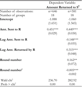
re-ciprocated by higher amounts returned in dyadic exchange arrangements. In Table 1, we report the
results from several random-effects Tobit regressions, where the dependent variable is the amount
returned by Receiver.8 The first regression has the amount sent by Sender as the only independent
variable and we find that the Receiver returns approximately 45% of an extra dollar received. This
result is robust once we add variables in the specification to capture the Receiver’s homegrown altruism
(amount returned by the same Receiver the previous period to a different Sender), an attempt by the
Receiver to induce more generosity if the period before the Sender had sent a smaller amount (the
amount received the period before from a different Sender), and time trends (round number and its
square allowing for a nonlinear time trend). The results show that these additional regressors are all
highly significant. Tables 5–7 report that Senders on average send $6.45 out of their $10 endowment,
and Receivers return about $9 (or 39.43%).
6.2
1S-2R
Given CCH, we would expect to observe downstream competition in [1s-2r] with full information
flow. That is because we would expect to find (i) evidence of relativized trust; and (ii) evidence
that that relativized trust is exploited to crowd-in higher returns. It is a relativized measure of trust
that Receiver behavior depends on, and it depends on it by being crowed-in toward off-equilibrium
cooperative behavior. And, if CCH is false, then we would expect either no differential evidence of
relativized trust or no differential evidence of crowding-in across information conditions.
First we examine the extent to which Receivers’ choice behavior depends on trustA and trustB;
that is, for example, whetherYA depends onXA−XB. This, of course, is exactly what is predicted
by a model of relativized trust: since trustA depends onXA−XB, and given the general result that
returns increase as level of trust increases, we would expectYA to increase as XA−XB increases.
Similarly for ReceiverB: YB should increase asXB−XAincreases. But this dependence is predicted,
given CCH, only under full information flow; under partial information flow, no such dependence is
expected since neither Receiver knowsXA−XB and so neither knows trustA/B.
In Table 2, we report the results from several random-effects Tobit regressions. The first two
regressions estimate the effects separately by information condition, where the dependent variable is
the amount returned by Receiveri.9 The two independent variables are amount sent toiand amount
sent to the other Receiver. Under partial info, the amount returned depends only on the amount
sent to Receiveri and not on the amount sent to Receiver−i (p = 0.000 and 0.599, respectively).
Approximately 47% of each unit received is returned to the Sender. Underfull info, it is also the
case that the coefficient on the amount sent to Receiveri is significant (p = 0.000); approximately
44% of each unit received is returned to Sender. Additionally, the coefficient on the amount sent to
Receiver−i is negative and significant (p = 0.067), indicating that Receiver i discounts the level of
generosity of the Sender if she observes increasing generosity toward Receiver−i. The result confirms
the prediction that Receivers use a relativized version of trust to determine the level of reciprocity
when the information is available to do so.
This result is robust. The third and fourth model specifications add a series of independent variables
to control for the effects of amounts sent to the Receiver by another Sender in the previous period,
a Receiver’s homegrown altruism, and time trends. There is strong evidence that all three have
significant effects in both information conditions: Receivers adjust to the amount previously sent by
returning more this period if they received a smaller amount the previous period, the Receivers exhibit
homegrown altruism by returning more this period if they had returned more the previous period, and
the time trend shows a non-linearity effect. Once controlling for these variables, underfull info, the
negative reaction to the amount sent by Sender to Receiver−i is still negative and weakly significant
(p= 0.10).
The final regression in Table 2 has as the dependent variable the difference in amounts returned
between Receivers A and B to the same Sender,YA−YB. The independent variables are the difference
in the amounts sent, a dummy for the information treatment, an interaction term between information,
the difference in the amounts sent, lags on the differences, and time trends. The results show that
the difference between the amounts sent,XA−XB, is an highly significant factor: about 42% more
is returned to the Sender for each unit sent to the Receiver in excess of what sent to Receiver−i
(p=.000). Moreover, the interaction term of information treatment with the difference in amounts
sent is highly significant, indicating that – when Receivers have information about what was sent to
the other at the time they make their return decision – they strictly compare to determine how much
to return (p= 0.027). This is clear evidence that Receivers utilize a notion of relativized trust.
By itself, the fact that Receiver behavior depends on a relativized measure of trust does not support
CCH. For that we need to see, in addition, that return behavior is more cooperative when information
about the bargaining environment is full. Then we will have evidence that (i) return behavior depends
on comparative information about trustA/B, and (ii) that the behavior on the long-side of the market
is crowded-in. So, accordingly, we examine the extent to which information crowds-in cooperation by
the Receivers. Here we see that, in fact, it does.
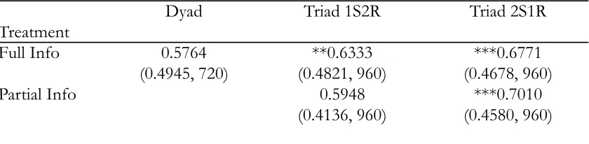
We can distinguishstrong andweak reciprocity: a response (return amount) by a Receiver signals weak reciprocity if the amount returned is not less than the amount invested; it signals strong
reci-procity if it is greater. We focus on the case of strong recireci-procity since it provides the strongest test
for CCH. Table 3 reports relative frequencies of (strong) reciprocity – i.e., the relative frequency of
returnsYi such thatYi> Xi – in the 2-node network and [1s-2r] under both information conditions.
For the dyad, it is approximately 57% and is not significantly different from [1s-2r] under partial info
suggesting higher rates of (strong) reciprocity by Receivers A and B over their counterparts in the
2-node network (p= 0.0180).
6.3
2S-1R
Given CCH, we would expect to observe upstream competition in [2s-1r] with full information flow.
That is because we would expect to find (i) evidence of relativized trust; and (ii) evidence that
that relativized trust is exploited to crowd-in higher transfers. It is a relativized measure of trust
that Senders’ behavior depends on, and it depends on it by being crowed-in toward off-equilibrium
cooperative behavior. And, if CCH is false, then we would expect either no differential evidence of
relativized trust or no differential evidence of crowding-in across information conditions.
First, we look to see whether Receiver behavior depends on relative investments. That is, we see
whether Yα (Yβ) depends on both Xα and Xβ instead of just Xα (Xβ). We find evidence for this
hypothesis.
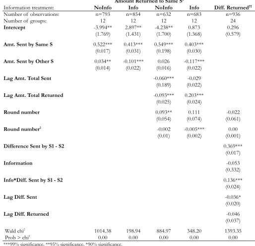
In Table 4, we report the results from several random-effects Tobit regressions. The first two
regressions estimate the effects separately by information condition, where the dependent variable is
the amount returned by the Receiver to Senderi; the two independent variables are amount sent by
Senderi and the amount sent by Sender−i.10 Our results show that in both information conditions,
as the amount sent by Senderi increases the amount returned to Senderiby the Receiver increases:
52% inpartial infoand 41% infull info of the gains from exchange are returned to the relevant
Sender. This is consistent with the body of evidence from investment game experiments.
The more important result is that, underfull info, Receivers continuously compare across Senders
and send approximately10% less to Senderi if Xi < X−i (p= 0.022). Under partial info, on the other hand, whennoinformation is available to Senderiregarding Receiver’s return to Sender−i, the Receiver rewardsislightly more – about 3% – the more she gets from the other Sender (p= 0.014).
These results suggest of an intention by the Receiver to indicate to the stingier Sender that he has
been punished and the more generous Sender has been rewarded.
The third and fourth model specifications in Table 4 add a series of independent variables to control
for the effects of total amount sent to the Receiver in the previous period, a Receiver’s homegrown
altruism, and time trends. Underpartial info, the Receiver returns about 55% of the gains from
exchange and underfull info returns a smaller percentage, approximately 40%. The positive and
10The censoring is between 0 and the amountXsent by Sender
significant coefficients found for the lag amount returned confirm the homegrown preferences toward
altruism already uncovered in the other networks. Interestingly, once controlling for these variables,
underfull info, the contemporaneous negative reaction to the amount sent by the other Sender is
still highly significant, with the Receiver penalizing Senderi by returning 10% less for each additional
dollar sent by Sender−i above what Senderi sent (p= 0.000).
The final regression we report in Table 4 has as the dependent variable the difference in amounts
returned by the Receiver to Sender αand Senderβ (Yα−Yβ). The difference between the amounts
sent by the two Senders has a significant effect (p= 0.075). Additionally, the interaction effect of the
information condition with the difference in the amount sent is highly significant (p= 0.000).
Under full infothe Receiver discriminates based on Senders relative investment. Senders learn
about this over time, triggering an arms race on high transfers. In 65% of the triads,Xα=Xβ. That
is, Senderα and Sender β make the same investment choice, even though they make those choices simultaneously when they do not have access to the investment choice of each other. In these cases, the
average amount sent is nearly the entire endowment, $9.23. When everyone invests almost all of the
endowment, there is little room to discriminate between them. However, inpartial info, only 46%
of the triads have equal investment levels and in these cases the average amount sent is much lower,
$6.20. This increase in competition occurs when the Senders receive information about what the other
Sender sent and what the Receiver returned to the other. This information about today’s interaction
leaves its mark on tomorrow’s behavior. The average amount sent is significantly higher—about 17%
higher—underfull info; otherwise the rate is the same as in the dyad (see Figure 1 and Table 5). As
a result, trustworthiness is higher underfull infoin both absolute amount and in terms of proportion
returned (see Tables 6A and 6B); the rates are not significantly different from the dyad underpartial
info.
These results confirm the CCH for information crowding-in cooperation on the long-side of the
market. Each Sender knows the level of trustα and trustβ, and each also knows Receiver’s reaction
to those levels. Consistent with the large body of investment game results, we see that Receiver
reciprocates a trusting Sender in this network. Further, Receiver responds differentially to differences
between trustα and trustβ. Seeing this, the Senders compete for the attention of the Receiver: we
have the predicted arms race in transfers. But in the same network with only partial information flow,
Receiver’s differential responses to Sender αand Sender β cannot be traced to differences in trustα
ensuing arms race, and we see less cooperative behavior on that side of the market.
6.4
Efficiency and Profits
In this last section on experimental results, we briefly discuss the impact of the observed behavior
on two important market features, efficiency (i.e., degree of realized surplus) and profits (i.e., final
distribution of that surplus). See Tables 6 and 7. In the baseline 2-node network, overall efficiency
is only 82.2%; on average, Senders earn $11.60 and Receivers earn $21.30 (including the initial $10
endowment).11 The [1s-2r] network is the most efficient at a rate of almost 94% and is independent of
flow of information as the rates of trust are high in both information conditions; interestingly, Senders
end up faring significantly better under full info than partial info, whereas Receivers, due to
the competition, fare significantly worse underfull infothan under partial info.12 The [2s-1r]
network does not generate efficiency gains over the baseline with an overall efficiency of approximately
82%; however, full info is significantly more efficient than partial info due to higher rates of
trust.13 In terms of profits, the Senders and Receivers fare better than under the baseline network.
7
Conclusions
We utilize networked versions of the investment game to explore how competition and cooperation
interact in more realistic bargaining environments, focusing on 3-node networked markets. The level
of competition in these markets is a function of the particular network structure and the level of
information available to the parties in the exchange.
Once we consider networked bargaining, we have to also consider whether standard behavioral
measures of trust in these environments are adequate. Does amount sent still carry that signal, or
do we need to know who sent it, or to whom they sent it? We described two plausible models of
trust, absolute and relativized. We have given a simple picture of a relativized model, and used it to
generate our main empirical hypothesis – that information crowds-in cooperation on the long-side of
the market.
Our findings suggest two related conclusions which support the Competition for Cooperation
Hy-pothesis. First, we find evidence that in networked bargaining, both in models of upstream and
11Efficiency is the ratio of the profits of the agents to the potential surplus available plus the endowment of the
Receiver(s). For the baseline: x40+y ×100
12For the [1s-2r]: x+yA+yB
50 ×100
13For the [2s-1r]: xα+xβ+y
downstream competition, it is relativized and not merely absolute trust measures that are operative.
Second, we find that when information flows fully in an environment, the network and relativized
trust measure are exploited to crowd-in cooperation on the long-side (competitive) of the market. In
our 3-node networks with downstream competition, this manifests itself in increasing returns. In our
3-node network with upstream competition, we instead see that Receivers – under full information
only – treat different Senders differently, and that this triggers an arms race on investments on the
Number of observations:
n=646
n=581
Number of groups
18
18
Intercept
-1.088
-1.060
(1.651)
(1.565)
Amt. Sent to R
0.451***
0.449***
(0.029)
(0.030)
Lag Amt. Sent to R
-0.148***
(0.035)
Lag Amt. Returned by R
0.315***
(0.048)
Round number
0.162**
(0.072)
Round number
2-0.005***
-0.002
Wald chi
2236.70
282.92
Prob > chi
20.00
0.00
***99% significance, **95% significance, *90% significance. †
Censored lower limit= 0; upper limit = Amount Sent by S1
[image:24.612.172.447.104.394.2]Amount Returned to S
†Diff. Returned†† Information treatment: NoInfo Info NoInfo Info
Number of observations: n=829 n=774 n=710 n=630 n=489
Number of groups: 24 24 24 24 24
Intercept -1.915** -0.315 -1.223 -0.24 0.0597
(0.858) (0.713) (0.996) (0.903) (0.786)
Amt. Sent to R Self 0.469*** 0.442*** 0.450*** 0.492***
(0.020) (0.022) (0.021) (0.025)
Amt. Sent to R Other 0.011 -0.043* -0.026 -0.042*
(0.020) (0.024) (0.021) (0.026)
Lag Amt. Sent to R Self -0.102*** -0.106***
(0.029) (0.032)
Lag Amt. Sent to R Other 0.004 0.006
(0.020) (0.025)
Lag Amt. Returned by R Self 0.224*** 0.208***
(0.045) (0.048)
Round number 0.077** 0.050 -0.075
(0.037) (0.048) (0.062)
Round number2
-0.003*** -0.003*** 0.002 (0.001) -0.001 (0.002)
Difference Sent to R1 - R2 0.421***
(0.024)
Information 0.252
(0.854)
Info*Diff. Sent to R1 - R2 0.083**
(0.038)
Lag Diff. Returned 0.130***
(0.047)
Lag Diff. Sent -0.057**
(0.028)
Wald chi2 985.33 726.84 1118.11 809.95 631.99
Prob > chi2
0.00 0.00 0.00 0.00 0
***99% significance, **95% significance, *90% significance.
†
Censored lower limit= 0; upper limit = Amount Sent by S to R Self
††
[image:25.612.84.563.110.617.2]Censored Regression. Lower limit=0 - Amount Sent to R2; upper limit = Amount Sent to R1
Table 2: Triads1S2R - Random-effects Tobit Regressions
Table 3. Relative Frequencies of Strong Reciprocity: Y > X
Dyad
Triad 1S2R
Triad 2S1R
Treatment
Full Info
0.5764
**0.6333
***0.6771
(0.4945, 720)
(0.4821, 960)
(0.4678, 960)
Partial Info
0.5948
***0.7010
(0.4136, 960)
(0.4580, 960)
Notes: Standard deviations and number of observations are reported in parentheses
Superscripts
***report Mann-Whitney results.
***
Information treatment:
NoInfo
Info
NoInfo
Info
Diff. Returned
††Number of observations:
n=793
n=854
n=632
n=683
n=936
Number of groups:
12
12
12
12
24
Intercept
-3.994**
2.897**
-4.238**
0.873
0.296
(1.769)
(1.431)
(1.700)
(1.368)
(0.579)
Amt. Sent by Same S
0.522***
0.413***
0.549***
0.403***
(0.017)
(0.031)
(0.198)
(0.030)
Amt. Sent by Other S
0.034**
-0.101***
0.026
-0.117***
(0.014)
(0.022)
(0.016)
(0.022)
Lag Amt. Total Sent
-0.060***
-0.029
(0.189)
(0.022)
Lag Amt. Total Returned
-0.093***
0.203***
(0.025)
(0.024)
Round number
0.093**
0.111
-0.022
(0.054)
(0.074)
(0.061)
Round number
2-0.002
-0.005***
0.00
(0.01)
(0.002)
(0.001)
Difference Sent by S1 - S2
0.369***
(0.017)
Information
-0.053
(0.332)
Info*Diff. Sent by S1 - S2
0.136***
(0.024)
Lag Diff. Sent
-0.036*
(0.020)
Lag Diff. Returned
-0.046
(0.037)
Wald chi
21014.38
198.94
884.97
348.20
1393.35
Prob > chi
20.00
0.00
0.00
0.00
0.00
***99% significance, **95% significance, *90% significance.
†
Censored lower limit= 0; upper limit = Amount Sent by Same S
††
[image:27.612.83.597.124.619.2]Censored Regression. Lower limit=0 - Amount Sent by S2; upper limit = Amount Sent by S1
Table 4: Triads 2S1R - Random-effects Tobit Regressions
Dependent Variable:
Table 5. Trust
Dyad
Treatment Amount Sent Tot. from S Avg. to Each R Tot. from S!&S" Avg. from Each S
Full Info 6.45 **
*** 8.43 *** *** 4.22 *** *** 14.55*** + *** 7.28*** +
(3.44, 720) (2.96, 480) (3.04, 960) (5.08, 480) (3.46, 960)
Partial Info ***
*** 8.72 *** *** 4.36 *** *** 12.46*** + 6.23 *** +
(2.46, 480) (2.76, 960) (6.20, 480) (3.82, 960)
Overall 6.45 ***
*** 8.58 *** *** 4.29 *** *** 13.51 *** 6.75
(3.44, 720) (2.72, 960) (2.90, 1920) (5.76, 960) (3.68, 1920)
Notes: Standard deviations and number of observations are reported in parentheses Superscripts ***
report Mann-Whitney results. Subscripts *** report Panel results.
The **,*** at the left of the mean indicate signicant differences across network treatment with respect to the corresponding value for the dyad; at the right of the mean they indicate signicant differences within network across information treatment.
Triad 2S1R Triad 1S2R
***
p#0.01; **
p#0.05; *
p!0.10; +
[image:28.612.86.577.305.486.2]p!0.15
Table 6A. Trustworthiness - Absolute Amount Returned by Receiver
Treatment Returned Returned Tot. to S Tot. to S Avg. per R Avg. per R Tot. from R Tot. from R Avg. to each S Avg. to each S
(zeros incl.) (zeros incl.) (zeros incl.) (zeros incl.) (zeros incl.)
Full Info 8.98 8.06 *
*** 11.19*** ** *** 10.38 + *** 6.43*** + *** 5.19 *** *** 21.85 *** ***
19.68*** *** 11.06***
* ***
9.84*** (7.50, 646) (7.61, 720) (5.24, 318) (5.80, 480) (4.82, 774) (5.02, 960) (12.72, 379) (12.69, 480) (7.18, 854) (7.61, 960)
Partial Info ***
9.82*** * *** 9.76 ** *** 5.65*** ** *** 4.88 *** *** 20.46 *** ***
16.09*** *** 9.74***
8.05*** (4.87, 362) (5.43, 480) (4.67, 829) (4.75, 960) (13.35, 349) (13.81, 480) (7.34, 793) (7.62, 960)
Overall 8.98 8.06 *
***10.46 *** ***10.07 ** ***6.03 ** ***5.03 *** ***21.18 ***
***17.88 ***10.42 *
***8.94 (7.50, 646) (7.61, 720) (5.09, 680) (5.62, 960) (4.75, 1603) (4.89, 1920) (13.04, 728) (13.38, 960) (7.29, 1647) (7.67, 1920)
Table 6B. Trustworthiness - Percentage Amount Returned by Receiver (of Amount Received from Sender) Dyad
Treatment % Returned % Tot. to S % Tot. to S % Avg. per R % Tot. from R % Tot. from R % Avg. to each S
(zeros incl.) (zeros incl.)
Full Info 39.43 40.46***
*** 40.51**** 39.55** ***44.69 ***45.52** ***44.74+ (27.35, 646) (17.08, 318) (17.45, 456) (23.22, 774) (23.36, 379) (24.72, 475) (25.45, 854) Partial Info **35.47***
*** 36.86**** **35.38** ***42.68 39.40** **40.29+ (15.65, 362) (17.48, 467) (21.79, 829) (22.87, 349) (23.67, 444) (23.98, 793)
Overall 39.43 37.81 38.67 37.39 ***
43.73 ***
42.56 ***
42.6 (27.35, 646) (16.51, 680) (17.56, 923) (22.58, 1603) (23.13, 728) (24.40, 919) (24.85, 1647)
Notes: Standard deviations and number of observations are reported in parentheses Superscripts *** report Mann-Whitney results. Subscripts
*** report Panel results.
The **,*** at the left of the mean indicate signicant differences across network treatment with respect to the corresponding value for the dyad; at the right of the mean they indicate signicant differences within network across information treatment.
***
p!0.01; **
p!0.05; *
p!0.10; +
p!0.15
Dyad
Triad 1S2R Triad 2S1R
[image:28.612.83.549.566.651.2]Triad 1S2R Triad 2S1R
Table 7. Profit
Treatment S R R net S Avg. R Avg. R net Avg. S R R net by S
Full Info 11.61 21.29 11.29 ***11.94**
+ ******17.46*** ******7.46*** +***12.56* ******33.98*** *11.99*** (6.06, 720) (8.09, 720) (8.09, 720) (4.41, 480) (6.00, 960) (6.00, 960) (6.13, 960) (14.16, 480) (8.29, 960)
Partial Info 11.05**
+ ******18.19*** ******8.19*** **11.81* ******31.30*** *10.65*** (4.59, 480) (5.77, 960) (5.77, 960) (5.51, 960) (12.79, 480) (7.89, 960)
Overall 11.61 21.29 11.29 *11.49
******17.83 ******7.83 ***12.19 ******32.64 11.32 (6.06, 720) (8.09, 720) (8.09, 720) (4.52, 960) (5.90, 1920) (5.90, 1920) (5.84, 1920) (13.55, 960) (8.12, 1920)
Notes: Standard deviations and number of observations are reported in parentheses Superscripts ***
report Mann-Whitney results. Subscripts *** report Panel results.
The **,*** at the left of the mean indicate signicant differences across network treatment with respect to the corresponding value for the dyad; at the right of the mean they indicate signicant differences within network across information treatment.
Triad 2S1R
***
p!0.01; **
p!0.05; *
p!0.10; +
p!0.15
Table 8. Efficiency - Realized Percentage of Theoretical Maximum Gains
Dyad
Triad 1S2R
Triad 2S1R
Treatment
Full Info
82.24%
******
93.73%
84.43%
***+
(17.22, 720)
(11.85, 480)
(14.52, 480)
Partial Info
******
94.87%
***78.47%
*** +(9.83, 480)
(17.71, 480)
Overall
82.24%
******
94.3%
*81.45%
(17.22, 720)
(10.90, 960)
(16.45, 960)
Notes: Standard deviations and number of observations are reported in parentheses Superscripts *** report Mann-Whitney results. Subscripts *** report Panel results.
The * at the left of the mean indicate signicant differences across network treatment with respect to the corresponding value for the dyad; at the right of the mean they indicate signicant differences within network across information treatment.
***
Figure 1:
!!!
Info - - - - NoInfo
Trust - 1S2R Total
0 1 2 3 4 5 6 7 8 9 10
1 23 45 67 8910 11 12 13 14 15 16 17 18 19 20 21 22 23 24 25 26 27 28 29 30 31 32 33 34 35 36 37 38 39 40 Round number A m o u n t sen t
Trust - 2S1R
0 1 2 3 4 5 6 7 8 9 10
12 34 56 78 910 11 12 13 14 15 16 17 18 19 20 21 22 23 24 25 26 27 28 29 30 31 32 33 34 35 36 37 38 39 40 Round number A m o u n t sen t
Trustworthiness - 1S2R Total
0 2 4 6 8 10 12 14
1 23 45 67 8910 11 12 13 14 15 16 17 18 19 20 21 22 23 24 25 26 27 28 29 30 31 32 33 34 35 36 37 38 39 40 Round number A m o u n t r et u r n ed
Trustwortiness - 2S1R
0 2 4 6 8 10 12 14
12 34 56 78 910 11 12 13 14 15 16 17 18 19 20 21 22 23 24 25 26 27 28 29 30 31 32 33 34 35 36 37 38 39 40 Round number A m o u n t r et u r n ed
Trustworthiness - 1S2R Total
0 10 20 30 40 50 60
1 23 45 67 8910 11 12 13 14 15 16 17 18 19 20 21 22 23 24 25 26 27 28 29 30 31 32 33 34 35 36 37 38 39 40 Round number % A m o u n t r et u rn ed
Trustworthiness - 2S1R
0 10 20 30 40 50 60
Figure 2:
!!!
!
1S1R
!
!!
!
!!
!
1S2R Tot
---
1S2R Each
!"!"!"!"
2S1R Each
Trust - Treatment Info
0 1 2 3 4 5 6 7 8 9 10
1 23 4 56 78 910 11 12 13 14 15 16 17 18 19 20 21 22 23 24 25 26 27 28 29 30 31 32 33 34 35 36 37 38 39 40 Round number A m o u n t sen t
Trust - Treatment NoInfo
0 1 2 3 4 5 6 7 8 9 10
1 23 4 56 78 910 11 12 13 14 15 16 17 18 19 20 21 22 23 24 25 26 27 28 29 30 31 32 33 34 35 36 37 38 39 40 Round number A m o u n t sen t
Trustworthiness - Treatment Info
0 2 4 6 8 10 12 14
1 23 4 56 78 910 11 12 13 14 15 16 17 18 19 20 21 22 23 24 25 26 27 28 29 30 31 32 33 34 35 36 37 38 39 40 Round number A m o u n t r et u r n ed
Trustworthiness - Treatment NoInfo
0 2 4 6 8 10 12 14
1 23 4 56 78 910 11 12 13 14 15 16 17 18 19 20 21 22 23 24 25 26 27 28 29 30 31 32 33 34 35 36 37 38 39 40 Round number A m o u n t r et u r n ed
Trustworthiness - Treatment Info
0 10 20 30 40 50 60
1 23 4 56 78 910 11 12 13 14 15 16 17 18 19 20 21 22 23 24 25 26 27 28 29 30 31 32 33 34 35 36 37 38 39 40 Round number % A m o u n t R et u r n ed
Trustwortiness - Treatment NoInfo
0 5 10 15 20 25 30 35 40 45 50