Imaging internal structure with electromagnetic induction tomography

IMTC 2006 – Instrumentation and Measurement Technology Conference

Sorrento, Italy 24-27 April 2006

Imaging Internal Structure with Electromagnetic Induction Tomography

X. Ma , A.J. Peyton , M. Soleimani and W.R.B. Lionheart

School of Electrical and Electronic Engineering, the University of Manchester, Manchester M60 1QD, UK, Phone: +44-161-3064808, Fax: +44-161-3064789, Email: [email protected]

2

School of Materials, the University of Manchester, Manchester, Manchester M60 1QD, UK

3

School of Mathematics, the University of Manchester, Manchester, Manchester M60 1QD, UK

Abstract – A particularly difficult case in electromagnetic induction tomography (EMT) is to image internal structure at the centre of the object space when the material at the outer regions is conductive. This is because the outer material acts as an electromagnetic screen, which partially excludes the magnetic field from the interior space and hence reduces the sensitivity at the centre.

In this paper, we propose a methodology to image the conductivity distribution of an annular object when internal conductive objects are present. Finite element simulations were carried out to investigate how sensor coil outputs change with factors such as the size of internal object with regards to the external one. Linear and non-linear image reconstruction methods are applied to the tomographic data that are collected from a newly developed EMT system and image results are given in the paper.

Keywords: magnetic induction, tomography, electromagnetic (EM), image reconstruction

I. INTRODUCTION

Electromagnetic induction tomography (EMT) images the spatial distribution of electrical conductivity and/or magnetic permeability inside a region of interest by obtaining a set of measurements using inductive coils that are distributed around the periphery. This form of tomography is non-intrusive and non-invasive such that the sensor coils are located external to the process or target. The systems operate by typically applying a set of interrogating field patterns to the region from different locations and directions. A number of measurements are taken by an array of sensors for each pattern. The measured data is then manipulated using mathematical inversion techniques to create an image of the internal object distribution. Areas of application for this technique include metal production, especially molten metal processes, and non-destructive testing [1-3]. Image resolution is poor compared to many other forms of tomography because of the limited number of excitation and detection coils and the nature of low frequency EM fields. However, for some of these applications it is sufficient simply to identify highly conductive regions within the object space such as whether a flow of molten is steel is biased towards one side of a delivery nozzle or is evenly distributed over the cross-section. In other cases, more information is required about the object distribution. A challenge in EMT is to image internal structure within complex object distributions.

A particularly difficult case is to discern internal structure at the centre of the object space when the material at the outer regions is conductive. This is because the outer material acts

as an electromagnetic screen, which partially excludes the magnetic field from the interior space and hence reduces the sensitivity at the centre. A practical example of this situation is distinguishing between an annular flow of liquid metal and one where the nozzle is completely filled. Other possible applications include non-destructive testing during the production of pipes to detect internal defects.

This paper considers a simple test case of an annular object with internal conductive objects.

II. METHODOLOGIES

A. Forward modelling

The forward problem in EMT is a classical eddy current problem. This problem can be formulated in terms of the

magnetic vector potential A for the sinusoidal waveform

excitation cases using complex phasor notation

s µ

1 _{A) iȦı A J}

( ’ u

u

’ (1)

where is electrical conductivity, µ is magnetic

permeability and Js is the applied current density in an excitation coil.

ı

The penetration of magnetic field below a test object

surface is described by the penetration depth G, which is

defined as į 1 ʌfµı, where f is the excitation frequency.

For non-magnetic, electrically conductive metals, the

permeability µ virtually equals to the permeability of free space, µ0, i.e., 4ʌ x 10-7 H/m. In fact, at an operating

frequency of 5 kHz, the penetration depth for copper (V | 58 MS/m) is about 0.93 mm which means that for a copper tube, for instance 2 mm thick, the field strength at the inside surface is roughly 16% of the field strength at the outside surface. Therefore, the field strength decreases significantly on the surface of an internal object when placed coaxially in the tube.

possibility of imaging annular objects, the 8-coil sensor array

was electromagnetically simulated with commercially

available software (Ansoft Cooperation’s Maxwell 3D EM field simulator). This software offered a piecewise solution to field problems by splitting the problem into a series of small tetrahedral elements over which the field values are approximated. The geometry being simulated includes an external tube of 140 mm diameter and 50 µm thick with circular rods placed inside the tube to represent internal structure. The objects were assigned the material property of copper.

Coil 8 Coil 6

Coil 2 Coil 4

Coil 1 Coil 5

Coil 3 Coil 7

X-Axis

Y-Ax

is

80 mm 80 mm

Fig. 1 Schematic diagram of sensor array used in the study

Simulations were carried out to assess how the coil outputs change with the diameter of the internal rod for a fixed size of the external tube with an excitation frequency of 5 kHz. Fig. 2 shows the changes in mutual impedance (imaginary part) with the radius of the internal rod measured on the coil 5

when coil 1 is excited. The background value is 0.0319 mȍ

when only the tube is present inside the object space. The quantization noise level of the system being simulated is 0.0024 mȍfor this opposite coil pair. This indicates that such a copper rod with a radius larger than 7.5 mm is resolved and therefore can be imaged when present inside a thin copper tube (140 mm diameter and 50 µm thick).

The relationship between them can be fitted numerically with a polynomial expression

2 5 4_{r 1.62 10 r}

10 9 . 3 0315 . 0

Z u u (2)

Therefore, the above quadratic expression can be used to approximately describe how the imaginary mutual coupling (Z) changes with the radius r of the internal rod.

B. Sensitivity analysis

If the total current in the excitation coil is , the

sensitivity of the induced voltage to the conductivity is [4-5]

0

I

0 k D

j i 2

k ij

I dv A . A

Ȧ ı

V :

³

w

w

(3)

where :D_k is the volume of the perturbation,A andA are

the solution of the forward solver when excitation coil ( ) is excited by

i j

i

0

I and sensing coil ( ) is excited withj unit

current.

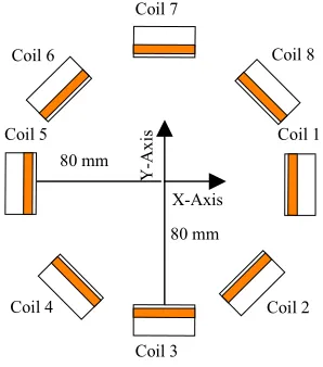
The sensitivity map changes with the background conductivity. Fig. 3 (upper) shows sensitivity plot of opposite

coils when a homogenous background (a cylinder of V = 0.4

S/m with 140 mm in diameter and 140 mm in length) is present. Fig. 3 (lower) is the sensitivity map between opposite coils when a tube with conductivity of 3 times bigger than the background is present, where the outer and inner radii of the ring object are 65 mm and 50 mm respectively. With a conductive background close to the surface, higher eddy currents are induced, which means that

those areas have higher sensitivity. In homogenous

background, the pixel intensity at the centre in the sensitivity

map is around 0.8 × 10-12 compared to 2.4 × 10-12 at the

surface; whereas in a background with a conductive tube present the pixel intensity at the centre is around 0.8 × 10-12 compared to 8 × 10-12 at the surface of the tube.

Obviously, the two sensitivity maps show that a much higher sensitivity contrast is produced in the object space when the background is conductive tube. As a result, a background with a conductive tube present raises a more ill-posed problem than a homogeneous background, making it difficult to image the internal structure.

Fig. 2 Changes in mutual coupling (imaginary part) of coil pairs with the size of internal rod when coil 1 is excited under the excitation

Fig. 3 Sensitivity in conductivity of opposite coils changes with different background, (upper) homogeneous background, and (lower) with a ring shape conductive object as a background. All dimensions

in X and Y directions are in m

C. Image reconstruction

In image reconstruction, both linear and non-linear algorithms were considered. The linear method is based on Tikhonov regularization, which uses a universal regularization technique for solving the ill-posed inverse problem in the following manner:

z J ) I µ J J (

x T 1 T (4)

where x is the image pixel vector, z is the measurement

vector, J is the sensitivity matrix (Jacobian matrix), Iis an identity matrix andP is the regularization parameter. In this single-step algorithm, sensitivity matrixJ was obtained with a direct measurement method [6].

The inverse problem in 3D eddy current imaging is both ill-posed and non-linear. As an iterative reconstruction algorithm, the regularised Gauss-Newton method starts with

an initial conductivity distribution . The forward problem

is solved using edge finite element method and the predicted voltages compared with the calculated voltages from the

forward model. The conductivity is then updated. The process is repeated until the predicted voltages from the finite element method agree with the calculated voltages from the finite element model to the required measurement precision [7]. The update formula at step n+1 is,

0 ı

)

ı

R R

Į

))

ı

( F z ( J ( ) R R

Į

J J (

ı

ı_{n1 n} T_{n n} 2 T 1 _nT _n 2 T _n (5)

where Jn is the sensitivity matrix updated with the

conductivityın, the forward solution F(ın ) is the predicted

voltages from the FE model with conductivityın. The matrix Į2

RTR is a regularization matrix, where R is a discrete

approximate to the Laplace operator. The parameter Į is a

regularisation parameter, which penalises extreme changes in conductivity removing the instability in the reconstruction, at the cost of producing artificially smooth images.

III. IMAGING RESULTS

A. EMT system

PC host computer Conditioning electronics unit Analogue/digital

connections via cables Excitation/detection signal connections

8-coil sensor array 45º

1

2 3 4 5

6 7

8

Fig. 4 Block diagram of the EMT system

Fig. 4 shows a block diagram of the main parts of the EMT system, which consists of a sensor array, a conditioning electronics unit and a PC host computer running with on-line data acquisition software. The system is controlled by a multifunction data acquisition board (ADLINK DAQ2205), which is housed inside the PC. The excitation coil is supplied from an a.c. current source with a peak current of 0.5 A. The conditioning electronics allows the driving/switching of the current source to each excitation coil in sequence, controls the gain selection for the induced voltage amplification, demodulates the induced voltage from the detection coils deriving both in-phase (real) and quadrature (imaginary) components.

Each coil is excited at an operation frequency of 5 kHz in turn as controlled by software and the induced voltages are then measured at the remaining coils. The imaginary parts of the induced voltage have been used for the conductivity image reconstruction, as they produce larger voltages, hence improve signal to noise ratio (SNR).

B. Imaging results

thick. The images of the tube with a copper rod of 35 mm, 19 mm and 9 mm in diameter inside are illustrated in figures 5(b), (c) and (d) respectively by using the linear algorithm in

equation (4). The regularization parameter P was chosen

5×10-5. Apparently, the presence of a smaller rod inside the tube will generate a smaller signal, which is superimposed to the much stronger signal generated by the tube, making it difficult to image the internal rod.

(a) (b)

(c) (d)

Fig. 5 Image reconstruction of copper tube with copper rod, (a) tube alone, (b) with a rod of 35 mm dia., (c) with a rod of 19 mm dia. and (d) with a rod of 9 mm dia. All dimensions in X and Y directions are in

mm

Fig. 6 shows some examples of annulus object with rods with conductivity close to that of steel in a case study of molten steel flow profiles during continuous casting. The first row in Fig. 6 represents the test arrangements, when one, two and three titanium rods and one aluminum plus three titanium rods are present inside an aluminum tube respectively. The

(a) (b)

(c) (d)

Fig. 6 Image reconstruction of aluminum tube with titanium rods, (a) one rod, (b) two rods, (c) three rods and (d) three titanium rods and one aluminum rod. All dimensions in X and Y directions are in mm

second row of the figure shows the reconstructed images and clearly the structure inside the tube cannot be distinguished. However, when the tube data is subtracted from these cases, as seen from the bottom of the figure, the internal rods are now clearly visible in each case. Even the more conductive aluminum rod can be resolved as in Fig. 6(d).

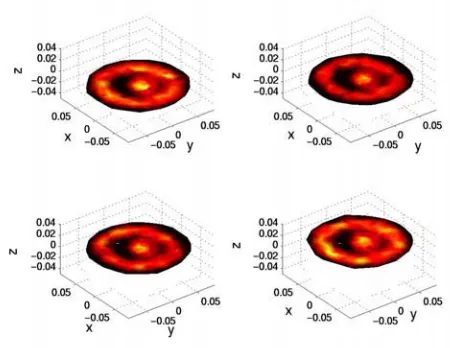
Fig. 7 Reconstruction of copper tube with a copper rod at different Z levels when the rod is placed in the centre. All dimensions in X and Y

directions are in m

tube shape than the single-step Tikhonov regularization. In

this study we choose the regularization parameter usingad

hoc methods and the regularization parameter Į in equation

(5) was chosen 10-5.

IV. CONCLUSIONS

This study has shown the potential of EMT for imaging coaxial annular objects. In particular, annulus object imaging is affected by a number of factors such as the relative size of the internal object, the compositions of external/internal objects, relative positions and excitation frequency being used. Example images have been presented, which show that under favorable conditions it is possible to image internal structure using just an 8-coil array, operating at a single excitation frequency. Further work is needed to advance the image reconstruction algorithms and exploit multiple frequency measurement techniques.

Fig. 8 shows the reconstructions at different Z levels when the internal rod is placed off the centre, e.g., a position at (5 mm, -5 mm). This position has a higher sensitivity than the centre and consequentially the quality of images shown in Fig. 8 is better than that in Fig. 7.

ACKNOWLEDGEMENT

The authors would like to thank UK Engineering and Physical Sciences Research Council (EPSRC) for their financial support of the project.

REFERENCES

[1] M. H. Pham, Y. Hua, and N. Gray, “Imaging the solidification of molten metal by eddy currents – Part 1”, Inverse Problems, vol. 16, pp. 469-482, 2000.

[2] M. H. Pham, Y. Hua, and N. Gray, “Imaging the solidification of molten metal by eddy currents – Part 1”, Inverse Problems, vol. 16, pp. 483-494, 2000.

Fig. 8 Reconstruction of copper tube with a copper rod at different Z levels when the rod is placed at (5 mm, -5 mm). All dimensions in X

and Y directions are in mm [3] X. Ma, A. J. Peyton, R. Binns and S. R. Higson, “Electromagnetic techniques for imaging the cross-section distribution of molten steel flow in the continuous casting nozzle”, IEEE Sensors Journal, vol. 5, no. 2, April 2005, pp. 224- 232.

The linear algorithm was run on a PC computer (AMD Athlon XP 1900+, 1.6 GHz CPU, 512 MB RAM) and required around 2 ms for an image production. As a single-step algorithm, Tikhonov regularization can be run in real-time.

[4] D. N. Dyck, D. A. Lowther and E M Freeman, “A method of computing the sensitivity of the electromagnetic quantities to changes in the material and sources”, IEEE Trans on Magn, vol. 3, no 5, Sep, 1994.

The edge FEM forward solver and the image reconstruction algorithm have been written in Matlab and run on a PC computer that has a 1.7 GHz Intel Pentium M processor and 512 MB RAM. The computational time for each nonlinear interaction of the inverse problem is around 26 minutes, which mainly covers the forward solver, Jacobian

matrix calculation and conductivity inversion.

Consequentially, this nonlinear method is used only for off-line data processing.

[5] H. Scharfetter, P. Riu, M. Populo and J. Rosell, “Sensitivity maps for low-contrast-perturbations within conducting background in magnetic induction tomography (MIT)”, Physiol Meas, 23: pp 195-202, 2002.

[6] X. Ma, A. J. Peyton, S. R. Higson, A. Lyons and S. J. Dickinson, “Hardware and software design for an electromagnetic induction tomography (EMT) system for high contrast metal process applications”, Meas. Sci. Technol., vol. 17, pp. 111-118, 2006. [7] M. Soleimani and W.R.B. Lionheart, A. J. Peyton and X. Ma, “A 3D