Munich Personal RePEc Archive
Can planners control competitive
generators?
Contreras, Javier and Krawczyk, Jacek and Zuccollo, James
Universidad de Castilla–La Mancha, Spain, Victoria University of
Wellington, New Zealand, Victoria University of Wellington, New
Zealand; supported by VUW FCA FRG-05 (24644).
30 August 2008
Can planners control competitive generators?
Javier Contreras, Jacek B. Krawczyk and James Zuccollo
Abstract
Consider an electricity market populated by competitive agents using thermal generating units.
Generation often emits pollution which a planner may wish to constrain through regulation. Furthermore,
generators’ ability to transmit energy may be naturally restricted by the grid’s facilities. The existence
of both pollution standards and transmission constraints can impose several restrictions upon the joint
strategy space of the agents. We propose a dynamic, game-theoretic model capable of analysing coupled
constraints equilibria (also known as generalised Nash equilibria). Our equilibria arise as solutions to
the planner’s problem of avoiding both network congestion and excessive pollution.The planner can
use the coupled constraints’ Lagrange multipliers to compute the charges the players would pay if the
constraints were violated. Once the players allow for the charges in their objective functions they will
feel compelled to obey the constraints in equilibrium. However, acoupled constraints equilibrium needs
to exist and be unique for this modification of the players’ objective functions ..[there was a “to” here,
incorrect?].. induce the required behaviour. We extend the three-nodedc model with transmission line constraints described in [10] and [2] to utilise a two-period load duration curve, and impose multi-period pollution constraints. We discuss the economic and environmental implications of the game’s solutions as we vary the planner’s preferences.
Universidad de Castilla–La Mancha, Spain; supported by the Spanish Ministry of Science and Technology through CICYT
grant ENE2006-02664
Victoria University of Wellington, New Zealand
Keywords: Coupled constraints games; generalised Nash equilibrium; deregulated electric in-dustry; electricity transmission, pollution constraints.
MSC: 91B32, 91B52, 91B76
I. INTRODUCTION
The aim of this paper is to examine the impact of pollution standards on electricity generators already subjected to grid facility restrictions.1
We consider an electricity market populated by competitive agents using thermal generating units. Such generation emits pollutants, on which a regulator (or planner) might wish to impose constraints. Transmission capacity for sending energy may naturally be restricted by the grid facilities. Both pollution standards and transmission capacity can be defined as constraints upon the joint strategy space of the agents.
We notice that the setup of the problem in this paper is similar to [25] and also to that discussed in [3]. Here, however, we utilise a two-period load duration curve and allow for the imposition of the environmental constraints on the two-period joint emissions. The analysis in [25] and [3] was confined to one period, while [25] did allow for no pollution constraints. We also make explicit in this paper the relationship between a solution to the problem and theweights, which the regulator may use to distribute the responsibility for the joint constraints’ satisfaction among the generators and/or periods.
We follow [21], [15], [2], [12] and [3], and use acoupled constraints equilibrium as a solution concept for the problem discussed. Under this solution concept the regulator can compute (for sufficiently concave games) the generators’ outputs that are both unilaterally non-improvable
1This paper draws from a conference paper [4] and from an earlier research report presented, under the same title, at the
School of Economics and Finance Workshop on “Optima and Equilibria in Problems of Energy Generation and Transmission”,
(Nash), and which satisfy the constraints imposed on the joint strategy space.2
If the regulator can impose penalties on the generators for violation of the joint constraints then the game becomes “decoupled” once the players incorporate the penalties in their payoff functions. If so, the players can compute and implement the coupled constraints equilibrium to avoid fines associated with both congestion and excessive pollution. These penalties that prevent excessive generation are computed by the regulator using the coupled constraints’ Lagrange mul-tipliers. However, for this modification of the players’ payoffs to induce the required behaviour, a coupled constraints equilibrium needs to exist and be unique (for a given distribution of the responsibilities for the joint constraints satisfaction, among the generators and periods.) A three-node bilateral market example, with a dc model of the transmission line constraints (described in [2]), possesses these properties and will be used in this paper to discuss and explain the behaviour of agents subjected to coupled constraints.
The analysis conducted in this paper should be particularly useful to regional governments interested in assessing the impact of environmental regulation on electricity generation. The case study considered shows significant market distortion and re-allocation of surplus as a result of the imposition of the various constraints. We also show that, by altering the degrees of responsibility for the joint constraints satisfactio namong the generators and periods, the planner may induce or “control” the generators to produce electricity at levels that correspond to a “socially acceptable” equilibrium.
For the results we use NIRA, which is a piece of software designed to min-maximise the Nikaido-Isoda function and thus compute a coupled constraints equilibrium (see [16]). We also notice that a coupled constraints equilibrium could be obtained3 as a solution to a
quasi-2Some authors call a coupled constraints equilibrium a
generalised Nash equilibriumand propose numerical solutions methods
based on variational inequality and/or linear complementarity formulations. Some, like [25], considered a generalised Nash
equilibrium problem (GNEP) in the context of a spatial oligopolistic electricity model and proposed a variational inequality
approach to determine a solution to the problem. Others, like [6] studied GNEPs via a variational inequality (VI) or a
quasi-variational inequality (QVI) reformulation and, more recently, [19] proposed some GNEP formulations of multi-leader-follower
games. Also, see footnote 4.
3
variational inequality4 (see [11], [19]) or gradient pseudo-norm minimisation (see [21], [7],
[8]).
What follows is a brief outline of what this paper contains. In section II a model of a bilateral electricity market game is presented. Section III briefly explains the idea of a coupled constraints equilibrium and the algorithm that will be used to find it. Sections IV, V and VI present the parameters of the case study and the results of our analysis. In section VII an economic interpretation is given to the results. The concluding remarks summarise our findings.
II. THE MODEL
A. A game with constraints
An electricity market is a system for effecting the purchase and sale of electricity, where the interaction between supply and demand sets the market price. Transactions are typically cleared and settled by the market operator or by a special-purpose independent entity charged exclusively with that function. If the offers by the generators and the demand bids are matched bilaterally then the market is known as bilateral. We focus on this type of electricity market in this paper. Transmission systems connect generators and consumer loads in an electricity network and they are operated to allow for continuity of supply. Transmission networks can experience bottlenecks; in addition, the authorities usually establish pollution limits on the generators’ emissions. These constraints limit the production of the generators and, consequently, their profits. In the following subsections we explain how the generators optimise their production and how the network and environmental constraints affect their profits in a coupled constraints game.
B. Generator’s problem
We assume no arbitrage (existence of marketers that can buy and sell power from producers and consumers) and a linear dc representation of the network.5
4
Some comparisons between NIRA and a method suitable for quasi-variational problems, which consists of a sequence of
solutions of linear complementarity problems, are provided in [17]. While both methods deliver the same solution, NIRA performs
less efficiently on the chosen (linear) example. As was observed in [24], NIRA is general being suitable for non-smooth games
and can be outperformed when games are “smooth”.
Each generator is maximising the sum of payoffs over a horizon T divided into periods of length∆t. The period length corresponds to the time within which the demand for electricity is considered constant according to the load duration curve6.
Each companyf = 1, . . . , F owns several generating unitsg = 1, . . . , Gdistributed throughout the network composed of nodes i, j = 1, . . . , N. The cost of running unit g that belongs to company f, placed at node i for period ∆t and whose power in this period is Pt
f gi MW, is
C(Pt
f gi)∆t. The maximum capacity of generator is Pf gi. Consumers buyqt
i MWh of energy at nodeiin periodt. At each node, linear demand functions are assumed to be of the form pt
i(σ t i) =a
t i− at i bt i σt
i where σti is the hourly demand in period t defined as σt
i =qit/∆t measured in MW (we will later refer to σit as demand for power). Price
pt
i(σit) is expressed in $/MWh and ati and bti are the price and power intercepts for (inverse) demand law at node i, respectively.
Energy st
f j MWh is sold by company f to consumers at node j in period t. Market clearing is such that the condition
fstf j = qjt holds. Also, an energy balance per period is imposed on each company:
i,gP t f gi∆t=
js t
f j. Given that (and remembering that demand is constant within∆t), each company f chooses generationPt
f gi and salesstf i to maximise profit ($), which is equal to revenue minus generation costs:
max j,t at j− at j bt j σt f j+
k=f
σt kj
st f j −
i,g,t
C(Pt f gi)∆
t (1)
subject to:
0≤Pt
f gi ≤Pf gi, ∀ nodes i, generators g, periods t
jstf j =
i,gPf git ∆t, for each firm f,∀ periods t
fs t
f j =qjt, for each node j,∀ periods t
⎫ ⎪ ⎪ ⎪ ⎬ ⎪ ⎪ ⎪ ⎭ (2)
We are interested in a non-cooperative solution to the game at hand. This means that we are looking for a distribution of generation and corresponding payoffs such that no player can improve his own payoff by a unilateral action. Bearing in mind that the solution is required to satisfy constraints, it will need to be understood as a “generalised” Nash-Cournot equilibrium as
6
The load duration curve is a curve of loads, plotted in a descending order of magnitude, against the time intervals for a
specified period. Load duration curves are profiles of system demand that can be drawn for specified periods of time (e.g., daily,
it is called in [19], or a coupled constraints equilibrium as we call it. We explain this concept in section III.
Notice that problem (1), (2) is time-decomposable because the generators cannot accumulate power across the periods. However, a generator problem would not enjoy this feature if an inter-temporal constraint were imposed.
C. Transmission constraints
The generating units and the nodes are connected by transmission lines, forming a network. The lines provide a path to transmit the power produced by the generators to the nodes for consumption. The power flowing through the lines is subject to thermal line limits. These limits are set in both directions of the flow in a line, which is why the absolute value is used in equation (3) below. To represent the topology of the network in this game it is necessary to select a node as the reference node. This is called the “slack” node or “swing” node (see [5] for details). The following equation expresses the flow going through the lines in period t as a linear function of the power injected at the nodes; this is called the dc approximation of the power flow:
Pti→j ≡
Bd·AT ·B−
1
·Pt, with |Pti→j| ≤Pi→j,7 (3)
where the variables and parameters are as follows:
Pti→j is a column vector whose number of rows is equal to the number of lines of the network. Each element represents the flow through the line i−j in period t, measured in MW.
Bd is the diagonal branch susceptance matrix, whose number of rows and columns is equal to the number of lines in the network. The diagonal terms of Bd are the susceptances of the lines (susceptance is the inverse of reactance). The reactances are expressed in per-unit
relative to the impedance base8 value.
7
Note that, throughout this paper, we use the notation|Pti→j|to denote a vector (or matrix) with each element being the
absolute value of the corresponding element ofPti→j. It is not intended to represent the norm of a vector.
8The
per-unit value of any quantity is defined as the ratio of the quantity to its base value, expressed as a decimal. See [22]
A is the node-branch incidence matrix; its dimensions are the number of nodes minus one (slack node) by the number of lines. The values of A are equal to+1 if the linei−j starts at node i, and −1 if it ends at node j.9
B is the diagonal node-to-node susceptance matrix; its dimensions are equal to the number of nodes minus one (slack node). The diagonal terms bii are equal to the sum of the susceptances of the lines that are connected to node i, and the terms bij are equal to the negative of the susceptances of the lines that connect node i and node j.
Pt is a column vector whose dimension is equal to the number of nodes minus one (the slack node). Its components are of the form (Pt
f gi−qti/∆t), representing the power in MW injected (generation minus demand) in each of the nodes in period t, except for the slack node.
Pi→j is a column vector whose number of rows is equal to the number of lines of the network. Each of its elements represents the thermal limit (maximum active power that can flow through a line) of a line in MW.
D. Pollution constraints
The thermal generation of electricity releases several contaminants into the atmosphere. The overall goal of reducing the emission of pollutants has to be expressed as a constraint for the overall production of all generating units. There are three main types of emissions: CO2, SO2
and NOx. The general expression of the pollution constraint for emissions of typeℓ is (see [20]):
h,t
∆t
αhℓ+βhℓPh+γhℓPh2
≤Kℓ, ℓ= 1, . . . L (4)
whereL can denote the number of noxious substances, for which restrictions are to be enforced or it may refer to the number of locations at which substance limits need to be observed.∆tis the duration in hours of periodt of the load duration curve andPh is the power output of generating unit h. The unit will be the g-th generator of firm f located at node i. However, for pollution generation and its constraint, the location of h relative to monitorℓ is relevant. Coefficientsαhℓ,
βhℓ, and γhℓ correspond to emissions discharged by unit h measured as pollution at location ℓ
9
(“type” ℓ). AmountKℓ is the maximum allowed pollution of type ℓ during all periods, usually measured in lb or Ton.
In (4), we have chosen to restrict the maximum allowed pollution of typeℓ duringall periods rather than per period, mainly to reflect the popular policy of many governments to delimit the allowable pollution in annual i.e., all-period terms. This introduces a dynamic aspect to the game: given a binding value of Kℓ the firms will consider tradeoffs between generating power in one period against generating it in another period so that the constraint is satisfied and their payoffs are maximised.
Each term of the left hand side of expression (4) can be interpreted as a steady-state solution to the partial differential equation describing the dispersion of pollution from a point source (see [1] for the integrated Gaussian puff diffusion model). In this paper, the coefficients of (4) have been calibrated following [20]).
The above constraint reflects the regulator’s concern for substanceℓconcentration at a selected (representative) location. More constraints of type (4) could be added to the problem formulation for more locations, at which the regulator would want to enforce compliance. If needed, the constraints can be defined as limits per periods and/or per generator, should such limits be known and adequate monitoring facilities exist.
III. CONSTRAINED EQUILIBRIA
A. Coupled constraints equilibria
A coupled constraints equilibrium (CCE) is an extension of a standard Nash equilibrium in which players’ strategy sets are allowed to depend upon other players’ strategies. Coupled constraints equilibria are also known as generalised Nash equilibria (compare footnote 2). The competition between electricity generating firms subject to constraints described above in section II is an example of such a problem. Analytical solutions to CCE problems are not normally possible so section III-B describes a numerical method for solving some such problems.
In our problem there are two such sets of coupled constraints: the line constraints and the environmental constraints. In both cases a limit is placed on a measurable variable — the flow of electricity through a particular line or the ambient pollution levels — and the actions of the players are constrained to jointly satisfy these limits.
In these games the constraints are assumed to be such that the resulting collective action set
X is a closed convex subset of IRm. If Xf is player-f’s action set, X ⊆ X1 × · · · ×XF is the collective action set (where X = X1× · · · ×XF represents the special case in which the constraints are uncoupled).
Consider the solution to this game represented by the collective action x∗ where players’ payoff functions, φf, are continuous in all players’ actions and concave in their own action10. The Nash equilibrium can be written as
φf(x∗) = max x∈X
φf(yf|x∗) (5)
where yf|x∗ denotes a collection of actions where thefth agent “tries” yf while the remaining agents continue to play the collective action x∗. Note that x∗ is a column vector with elements
xg, g = 1,2, . . . , f −1, f + 1, . . . , F. At x∗ no player can improve his own payoff through a unilateral change in his strategy so x∗ is a Nash equilibrium point. If X is a closed and strictly convex set defined through coupled constraints (like (4)) then x∗ is a CCE.
B. NIRA
Games with coupled constraints rarely allow for an analytical solution and so numerical methods must be employed. Here we use a method based on the Nikaido-Isoda function and a relaxation algorithm (hence the name: NIRA).
1) The Nikaido-Isoda function: This function is a cornerstone of the NIRA technique for solving games for their CCE. It transforms the complex process of solving a (constrained) game into a far simpler (constrained) optimisation problem.
In the remainder of this section (i.e., section III), we are indexing a player’s action, payoff, weight,etc. by the sole indexf. If the players’ responsibilities are distributed non-equally among periods t, then all these variables should be indexed by f and t. We will do so in sections IV
10In our study, the payoff functionφ
and V where the game solutions are computed and interpreted. Here, however, for clarity of notation and interpretations of the Nikaido-Isoda function we use the single index.
Definition III.1. Letφf be the payoff function for playerf, X a collective strategy set as before
and rf >0 be a given weighting11 of player f. The Nikaido-Isoda functionΨ : X×X → IR
is defined as
Ψ(x,y) =
F
f=1
rf[φf(yf|x)−φf(x)] (6)
Result III.1. See [23].
Ψ(x,x)≡0 x∈X. (7)
Each summand from the Nikaido-Isoda function can be thought of as the improvement in payoff a player will receive by changing his action fromxf toyf while all other players continue to play according to x. Therefore, the function represents the sum of these improvements in payoff. Note that themaximum value this function can take, for a givenx, is always nonnegative, owing to Result III.1 above. The function is everywhere non-positive when either x or y is a Nash equilibrium point, since in an equilibrium situation no player can make any improvement to their payoff. Consequently, each summand in this case can be at most zero at the Nash equilibrium point [15].
We observe that the “sum of improvements” inΨdepends on the weighting vectorr= (rf)f∈F. Consequently, a manifold of equilibria indexed by r is expected to exist. However, for a given
r and diagonal strict concavity of
f∈F rfφf(xf), uniqueness of equilibriumx∗ is guaranteed, see [21] and [9]. Also, notice that according to the convergence theorem ([23], [15]), if its assumptions are fulfilled, then NIRA converges to the unique equilibrium, for the value ofr that was used in the definition of Ψ.
When the Nikaido-Isoda function cannot be made (significantly) positive for a given y, we have (approximately) reached the Nash equilibrium point. This observation is used to construct
11
The weights can be viewed as a political instrument the regulator might use to distribute the responsibility for the joint
constraints’ satisfaction, among the generators and periods. If the players’ responsibilities are distributed in periodstnon-equally,
then the weights, actions, payoffsetc. becomert f, x
t f, φ
t
a termination condition for the relaxation algorithm, which is used to min-maximiseΨ. An ε is chosen such that, when
max
y∈IR mΨ(x
s
,y)< ε, (8)
(where xs is the s-th iteration approximation of x∗) the Nash equilibrium would be achieved to
a sufficient degree of precision [15].
The Nikaido-Isoda function is used to construct the optimum response function. This function is similar to the best response function in standard non-cooperative game theory. It defines each player’s optimal action to maximise his payoff given what the other players have chosen. The vector Z(x) gives the ‘best move’ of each player when faced with the collective action x. It is at this point that the coupled constraints are introduced into the optimisation problem. The maximisation of the Nikaido-Isoda function in equation (9) is performed subject to the constraints on the players’ actions.
Definition III.2. The optimum response function at point x is
Z(x)∈arg max
y∈X
Ψ(x,y). (9)
2) The relaxation algorithm: The relaxation algorithm iterates the functionΨto find the Nash equilibrium of a game. It starts with an initial estimate of the Nash equilibrium and iterates from that point towards Z(x) until no more improvement is possible. At such a point every player is playing their optimum response to every other player’s action and the Nash equilibrium is reached. The relaxation algorithm, when Z(x) is single-valued, is
xs+1 = (1−αs)xs+αsZ(xs) 0< αs ≤1 (10)
s = 0,1,2, . . .
From the initial estimate, an iterate steps+1is constructed by a weighted average of the players’ improvement point Z(xs) and the current action pointxs. Given special concavity assumptions (see [23], [15]), this averaging ensures convergence to the Nash equilibrium by the algorithm.
C. Existence and uniqueness of equilibrium points
NIRA algorithm converges to a single equilibrium point it would be nice if that equilibrium could be shown to be unique. The conditions for existence and uniqueness for games with coupled constraints are more intricate than those for games with uncoupled constraints. It is known that every concave n-person game with uncoupled constraints has an equilibrium point [21]. The equivalent definition for a game with coupled constraints relies upon the notion of a weakly convex-concave function12
D. Enforcement through taxation
Once a CCE, x∗, has been computed it is possible to create an unconstrained game which
has x∗ as its solution by a simple modification to the players’ payoff functions. For example, a
regulator may compute thatx∗ is the CCE of a game involving the desired constraints on agents’
behaviour. He may then wish to induce the players to arrive at this point through a scheme of taxation that modifies their payoff functions. This can be achieved by the use of penalty functions that punish players for breaching the coupled constraints.
Penalty functions are weighted by the Lagrange multipliers obtained from the constrained game. For each constraint, players are taxed according to the function
Tℓ,f(λ, rf,x) =
λℓ
rf
max(0, Qℓ(x)−Qℓ) (11)
whereλℓ is the Lagrange multiplier associated with the ℓth constraintQℓ(x)may be the amount of pollution as described by the left hand side of (4), or of the transmitted power as in (3), while
Qℓ, ℓ = 1,2, . . . L denote the corresponding limits (L is the total number of constraints); x is the vector of players’ actions, rf is player f’s weight that defines their responsibility for the constraints’ satisfaction.
If the weights r were identical [1,1, . . .1] (see [3]) then the penalty term for constraint ℓ is the same for each player f
Tℓ,f(λ,1,x) =λℓmax(0, Qℓ(x)−Qℓ).
Hence, if the weight for player f is for example rf > 1 and the weights for the other players were 1,1, . . .1, then the responsibility of player f for the constraints’ satisfaction is lessened.
12
A weakly convex-concave function is a bivariate function that exhibits weak convexity in its first argument and weak
Obviously, if the players’ responsibilities are distributed in periods t non-equally, then the weights, as well as the other variables, need the other index t.
The players’ payoff functions, so modified, will be
φf(x) =Rf(x)−Cf(x)−
ℓ
Tℓf(λ,r,x) (12)
where Rf and Cf are firm f’s revenue and cost functions respectively. Notice that under this taxation scheme the penalties remain “nominal” (i.e., zero) if all constraints are satisfied.
The Nash equilibrium of the new unconstrained game with payoff functions φ is implicitly defined by the equation
φ(x∗∗) = max
yf∈IR
+φ(yf|x
∗∗
) ∀f, (13)
(compare with equation (5)). For the setup of the problem considered in this paper x∗ = x∗∗.
That is, the CCE is equal to the unconstrained equilibrium with penalty functions for breaches of the constraints, weighted by the Lagrange multipliers (see [15], [12] and [13] for a more detailed discussion).
IV. CASE STUDY
A. Without coupled constraints
The example is taken from [2] (originally, from [10]). Numerical data for the general formu-lation of the problem is as follows. The period of study is split into two sub-periods, weekdays and weekends, for which the demands for electricity are different. The periods account for
5·24h=120 h and2·24h=48 h per week, or in annual terms to 5/7 and 2/7 of the365·24 = 8,760h of an entire yeari.e., 6,257 h and 2,503 h , respectively. These periods correspond to the two parts, into which the load duration curve is divided. We assume that every hour within each period is identical in terms of demand for energy, sales, power generations, etc.
There are three nodes, i= 1, 2, 3, each of which has customers. Generation occurs only at nodes 1 and 2 and each pair of nodes is connected by a single transmission line. The demand functions (per hour) are: in period 1, p1
i(σ
1
i) = 40−0.08σ
1
i, for nodes i = 1, 2 and p
1 3(σ
1 3) =
32−0.0516σ1
3 $/MWh for node 3; in period 2, p 2
i(σ
2
i) = 30−0.06σ
2
i, for nodes i= 1, 2 and
p2 3(σ
2
3) = 24−0.0387σ 2
node 3. Firm’s 1 generator is placed at i= 1 and firm’s 2 ati= 2. Since each firm has only one generator we drop the i and g subscripts for brevity (e.g., Pt
f gi becomes Pft). Both generators have unlimited capacity and constant marginal costs MC1 = dC(P
1 1) dP1
1
= dC(P
2 1) dP2
1
= 15 for firm
1 andMC2 = dC(P 1 2) dP1
2
= dC(P
2 2) dP2
2
= 20for firm 2. The marginal costs are measured in $/MWh. The three lines have equal impedances of 0.2 p.u. The slack node is node 3.
Bearing in mind the general formulation of the generation game defined by the payoffs (1) and constraints (including coupled) (2)–(4) and the numerical values for the problem parameters as above, both firms solve the following optimisation problems:
Firm 1:
max
[40−0.08σ1 1]s
1
11+ [40−0.08σ 1 2]s
1
12+ [32−0.0516σ 1 3]s
1
13−15P 1
1 ·6,257+
[30−0.06σ2 1]s
2
11+ [30−0.06σ 2 2]s
2
12+ [24−0.0387σ 2 3]s
2
13−15P 2
1 ·2,503
(14)
Firm 2:
max
[40−0.08σ1 1]s
1
21+ [40−0.08σ 1 2]s
1
22+ [32−0.0516σ 1 3]s
1
23−20P 1
2 ·6,257+
[30−0.06σ2 1]s
2
21+ [30−0.06σ 2 2]s
2
22+ [24−0.0387σ 2 3]s
2
23−20P 2
2 ·2,503
(15)
P1 1∆
1
=s1 11+s
1 12+s
1
13, (16a) P2
1∆ 1
=s2 11+s
2 12+s
2
13, (16b) P1
2∆ 2
=s1 21+s
1 22+s
1
23, (16c) P2
2∆ 2
=s2 21+s
2 22+s
2
23, (16d) q1
1 =s 1 11+s
1
21, (16e) q2
1 =s 2 11+s
2
21, (16f) q1
2 =s 1 12+s
1
22, (16g) q2
2 =s 2 12+s
2
22, (16h) q1
3 =s 1 13+s
1
23, (16i) q2
3 =s 2 13+s
2
all s1 11, s
2 11, s
1 12, s
2 12, s
1 13, s
2 13, s
1 21, s
2 21, s
1 22, s
2 22, s
1 23, s
2 23,
P11→2, P 2 1→2, P
1 1→3, P
2 1→3, P
1 2→3, P
2
2→3, nonnegative,
where the decision variables of the generators (firms) are: s1 11, s
2 11, s
1 12, s
2 12, s
1
13 and s 2
13 for the
first generator, and s1 21, s
2 21, s
1 22, s
2 22, s
1
23 and s 2
23 for the second generator. As in section II-B, σt
i =qit/∆t.
The remaining variables are dependent on the decision variables. If the problem involves constraints then part of the solution will constitute the Lagrange multipliers that a regional regulator will be able to use to enforce the equilibrium (see section III-D).
B. Transmission line constraints
A constraint on transmission line capacity per period of the load duration curve is imposed as described in equation (3).13 The equations of the constraints in this example are
Bd·AT ·B−
1
·
⎛
⎝
P1 1 −q
1 1/∆
1
P1 2 −q
1 2/∆
1 ⎞ ⎠ ≤ ⎛ ⎜ ⎜ ⎜ ⎝
P11→2
P11→3
P12→3
⎞ ⎟ ⎟ ⎟ ⎠ . (18)
Bd·AT ·B−
1
·
⎛
⎝
P2 1 −q
2 1/∆
2
P2 2 −q
2 2/∆
2 ⎞ ⎠ ≤ ⎛ ⎜ ⎜ ⎜ ⎝
P21→2
P21→3
P22→3
⎞ ⎟ ⎟ ⎟ ⎠ . (19)
The values of the transmission line constraints are as follows:
Bd=
⎛
⎜ ⎜ ⎜ ⎝
5 0 0
0 5 0
0 0 5 ⎞
⎟ ⎟ ⎟ ⎠
, A=
⎛
⎝
1 1 0
−1 0 1 ⎞
⎠, B = ⎛
⎝
10 −5
−5 10 ⎞
⎠. (20)
Note that the first row of matrix A (whose dimension is: 2 nodes times 3 lines) expresses that node 1 is the starting node of lines 1–2 and 1–3, and the second row means that node 2 is the
13
For example, the first row ofP1
i→jis
P1
1→2= 0.66s 1 12/∆
1
+ 0.33s1 13/∆
1
−0.66s1 21/∆
1
−0.33s1 23/∆
1
. (17)
This indicates that the flow along the line from node1to node2in period 1 depends not only upon the quantity that is sold
ending node of line 1–2 and the starting node of line 2–3. Node 3 is the slack node for which there are no calculations, since it is the reference node.
The diagonal terms of B are computed as follows: b11is the sum of the two line susceptances
connected to node 1, likewise for the other diagonal term corresponding to node 2. The off-diagonal terms are the susceptances of the lines 1–2 and 2–1 (which is the same line), respectively. Substituting the matrices in (20) into equations (18) and (19), and choosing line limits
(25,200,200)′, gives this numerical expression for the line constraints in periods 1 and 2:
⎛ ⎜ ⎜ ⎜ ⎝
0.33 −0.33
0.66 0.33
0.33 0.66 ⎞ ⎟ ⎟ ⎟ ⎠ · ⎛ ⎝ P1 1 −q
1 1/∆
1
P1 2 −q
1 2/∆
1 ⎞ ⎠ ≤ ⎛ ⎜ ⎜ ⎜ ⎝ 25 200 200 ⎞ ⎟ ⎟ ⎟ ⎠ . (21) ⎛ ⎜ ⎜ ⎜ ⎝
0.33 −0.33
0.66 0.33
0.33 0.66 ⎞ ⎟ ⎟ ⎟ ⎠ · ⎛ ⎝ P2 1 −q
2 1/∆
2
P2 2 −q
2 2/∆
2 ⎞ ⎠ ≤ ⎛ ⎜ ⎜ ⎜ ⎝ 25 200 200 ⎞ ⎟ ⎟ ⎟ ⎠ . (22)
Pt1→3 andP
t
2→3 are set arbitrarily large such that they never bind. Because of this, our problem
can be considered to have only one coupled constraint on Pt
1→2. Lagrange multipliers are only
reported for this active constraint in the results below.
C. Environmental constraints
In this case study, an emission constraint is added to the problem formulation. As a result, the problem is set as in (14)–(16), where both firms have the same optimization functions as before, but, in this case, a new environmental constraint is added to the constraint set (16), so that:
6,257·[(20−0.4·P1
1 + 0.004·(P 1 1)
2
) + (22−0.3·P1
2 + 0.005·(P 1 2)
2
)]+
2,503·[(20−0.4·P2
1 + 0.004·(P 2 1)
2
) + (22−0.3·P2
2 + 0.005·(P 2 2)
2
)]≤2,190,000,
(23) where the maximum allowed emission is 2,190,000 lb. Note14. that (23) is applied to periods 1
and 2 simultaneously. Consequently, this constraint has a time coupling effect.
14We turn the reader’s attention to the fact that the function in expression (23) is quadratic so, the second superindex means
The annual emission limit assumes a constant hourly value of 250 lb/h that, multiplied by 8,760 hours, results in 2,190,000 lb per year.
D. What kind of stylised situation reflects the model
Our first generator is economically efficient and has good filters. The other generator is “outdated” and does not have good filters. The transmission line between the generators is due for an upgrade while the other lines are recently rebuilt and have a high transmission capacity. As judged by the nodal demand laws, the first two nodes represent localities with a mixture of industrial and domestic customers. The third node corresponds to a township or a conglomerate of rural customers whose demand for electricity is lower than in the first two localities.
As said earlier, the demand functions change depending on the period. It is assumed that the demand in weekdays (first period) is higher than the demand on weekends (second period).
The local regulator is concerned about pollution levels at some critical location (like a National Park) where a monitor is installed. The monitor is capable of detecting if the total annual pollution exceeds 2,190,000 lb, see condition (23). Presumably, the coefficients of the pollution function in this equation have been calibrated to reflect the emissions’ transportation process from each generator to the “critical” location.
The local environmental lobby group has managed to legislate that the limit of K = 2,190
klbsper year, measured at the “critical” location, has to be obeyed. The local regulator considers an introduction of a pollution charge to be paid by both generators should a violation of this constraint be detected.
The local regulator is interested to know what the generators’ reactions could be should the pollution charge become a reality. In particular, the regulator would like to know what energy prices can be expected after the introduction, whether the energy supply might be affected and in what way the region’s welfare may be influenced. The results presented below provide some answers to these questions.
V. SHARING THE CONSTRAINTS’ BURDEN IN SOLIDARITY
Here we show the equilibrium results for when all weights15 rt
f ≡ 1 i.e., the constraints’ burden is shared in solidarity. We anticipate that, at realising what impact the constraints on
the local economy might have, the regulator will try and test some measures to improve “social acceptability” of the equilibrium. Those measures will be described and analysed in section VI.
A. The results
As said earlier, the generation game (14), (15), (16) (with constraints (21),(22) and (23), if appropriate) satisfies the hypotheses of the convergence theorem (see [23], [15]) of the NIRA method. Consequently, we have used NIRA (described in section III-B) to obtain the game’s solutions16 reported fully in [4]. Here we completely present the base case results only, to show
all details of the solutions obtainable through NIRA, presumably important for the planner. We analyse the results for all cases using graphs and diagrams in section V-B.
1) Base case (i.e., no constraints):
The results of the application of NIRA to the game defined by (14)–(16) are shown in tables I and II. These tables have three or two rows of results: all first row’s numbers concern the first period, the second row’s refer to the second period. The third row (if appropriate) provides the sums for both periods.
We can read the energy demanded per node for the first period is: 1,173.18 GWh, 1,173.18 GWh, and 1,172.18 GWh and for the second period, 347.64 GWh, 347.64 GWh, and 291.05 GWh. As expected, the “weekend” demand is lower than the weekdays’; also, the third node (“rural”) consumes less energy than the other nodes.
Prices at the nodes, according to the linear demand functions, are: 25, 25, and 22.3 $/MWh for the first period and 21.66, 21.66 and 19.5 $MWh for the second period.
The flows’ absolute values per hour through the lines are: 73.96 MW, 130.65 MW, and 56.7 MW for lines 1–2, 1–3 and 2–3, in the first period and 94.31 MW, 105.29 MW, and 10.98 MW for lines 1–2, 1–3 and 2–3 in the second period.
Profits for the first period for firms 1 and 2 are 22.16 M$ and 4.57 M$, respectively; for the second period, they are 5.02 M$ and 232 k$, respectively. As expected, the first generator produces substantially more than the second. Total pollution is 4,627 klb. As no constraints are active the Lagrange multipliers for the line and environmental constraints are: λ1
L1 = λ 2
L1 =
16
We remind the reader that a solution (equilibrium) is a combination of the decision variables’ values such that the constraints
λE = 0(notice that we do not indexλE with time because this Lagrange multiplier corresponds to the intertemporary constraint (23)).
TABLE I
SALES,GENERATION AND TOTAL EMISSIONS IN THE BASE CASE
Sales by Firm 1
(1000MWh)
Sales by Firm 2
(1000MWh)
Generation by
Firms (1000MWh)
Emissions by
Firms (1000lb)
st
11 st12 st13 st21 st22 st23 P1t∆t P2t∆t E1t E2t
782.12 782.12 889.24 391.06 391.06 282.94 2453.5 1065.1 2992 724.6
278.11 278.11 291.05 69.53 69.53 0 847.3 139.1 858.4 52
1060.24 1060.24 1180.3 460.6 460.6 282.94 3300.8 1204.2 3850.4 776.6
TABLE II
ECONOMICS OF GENERATION IN THE BASE CASE PER HOUR PER PERIOD
Demand (MW) Prices ($/MWh) Profits ($/h)
σt
1 σ
t
2 σ
t
3 p
t
1 p
t
2 p
t
3 Π1 Π2
187.5 187.5 187.34 25 25 22.33 3542.2 730.51
138.89 138.89 116.28 21.66 21.66 19.5 2004.8 92.7
Flows for lines (MW) Lagrange multipliers Emission levels (lb/h)
1 – 2 1−3 2−3 λt
T λE Firm1 Firm2 Total
73.96 130.65 56.69 - - 478.18 115.81 593.99
94.31 105.29 10.98 - - 342.93 20.76 363.7
2) Generation under a transmission constraint:
For this example, a limit of 25 MW in the transmission capacity of the line that connects nodes 1 and 2 is imposed. As a result, the problem is set as in section V-A1 above with the addition of the constraints described in equations (18) and (19).
This generation game is a game with coupled constraints, among two non identical players (player 1 produces electricity more cheaply than player 2) where the constraints (21), (22) are binding.
3) Generation under an environmental constraint:
if the environmental constraint (23) was introduced (and the transmission line upgraded so that the line constraint became non-binding).
4) Generation under transmission and environmental constraints:
In this case study, both the 25 MW thermal limit of line 1–2 (equations (18) and (19)) and the emission constraints (equation (23)) are added to the basic problem formulation.
B. The discussion
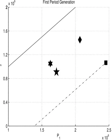
We have noticed that the imposition of constraints favours the second generator in that its share of production increases. This is shown in figure 1. The symbols in the figure correspond to the above four cases as follows:
1) square – no constraints (section V-A1);
2) diamond– transmission line constraint (section V-A2); 3) pentagram – environmental constraint (section V-A3); 4) hexagram – the two constraints jointly (section V-A4).
1 1.5 2 2.5
x 106 0
0.4 0.8 1.2 1.6
22x 10
6 First Period Generation
P1
P
2
4 6 8
x 105 0
200,000 400,000 600,000 800,000
Second Period Generation
P1
P
[image:21.612.87.283.392.637.2]2
All lines in figure 1 are angled at 45o. The solid ones go through the origin. If the generators were identical, the constraints would affect each them in the same way and the generation points would be on this line. Obviously, the generators in the case study are not identical. However, we notice that imposition of a constraint blurs the difference. This is visible from the diminishing distances of the generation points from the 45o line, after a constraint imposition.
The dash-dotted lines pass through the unconstrained generation point (square). They are drawn to help assess the distance of each generation point from the 45o line.
The overall result is that the constrained generation games increase the market share of firm 2 (the less efficient one). This can be qualified as market distortion. In particular, when a transmission constraint is the only restriction, the distortion concerns the generators rather than consumers; this is evident from the numerical results (see [4], omitted here) and shown in figure 6 in section VII-A. In case of the imposition of an environmental constraint (sole or joint with a transmission constraint) the prices rise substantially and the consumers’ surplus17 is diminished.
We will comment on this issue later also in section VII-A.
We conjecture that the market distortion due to constraints is unavoidable. If a line constraint is imposed on the flow through link 1–2, then (17) (in footnote 13) has to be satisfied. It is evident from (17) that, for this to happen, the sales by firm 2 at nodes one and two have to increase and those of firm 1 have to decrease. This explains the generation changes (in figure 1 from square to diamond) when a line constraint is imposed.
We can also observe the generation changes due to the imposition of an environmental constraint. In figure 1, the outputs “move” from square to pentagram. Generation by firm 1 diminishes substantially while that by firm 2 can increase (in period 2) or decrease a little (in period 1). In each period firm 2’s market share is greater than in the unconstrained case.
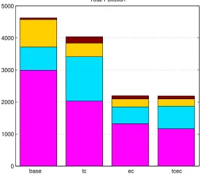
We observe in figure 2 that imposing a constraint changes the proportions, in which the firms contribute to the total pollution. In this figure, each bar represents the total pollution correspond-ing to the base game, transmission-constraint game (tc), environmental-constraint game (ec) and transmission-&-environmental-constraint game (tcec), respectively. The two bottom fields symbolise the first period’s pollution by firm 1 (bottom) and 2; the two top fields represent the
17Consumer surplus isCS=N i=1
q∗
i
2(ai−p
∗
i)whereqi∗andp∗i are the equilibrium quantity and price at nodeiandaiis
second period’s pollution by firm 2 (top) and 1.
0 1000 2000 3000 4000 5000
Total Pollution
[image:23.612.160.449.122.383.2]base tc ec tcec
Fig. 2. Total pollution in 1000lb.
The contributions are functions of the generation, see figure 3.
Given that firm 1 is more environmentally friendly (i.e., it emits less per unit of generation) it could be expected that, as the environmental constraint tightens, firm 1’s market share would increase. However, this is not what we observe in figure 1. As the environmental constraint is tightened, with or without a binding line constraint, the market share of the environmentally inefficient firm 2 increases. We conjecture that the source of this apparent anomaly are changes in the effective marginal costs TMCf under the imposition of constraints. In words, the firm’s
effective marginal cost isMCf whereMCf is firm’sf marginal cost dC(Pf) dPf
plus the marginal cost of the pollution constraints’ violation, which depends on the weightrt
0 50 100 150 200 250 300 350 400 0
50 100 150 200 250 300 350 400 450 500
Power [MW] emissions [lb]
0 50 100 150 200 250 300 350 400 0
50 100 150 200 250 300 350 400 450 500
Power [MW] emissions [lb]
[image:24.612.190.429.75.322.2]firm 1 firm 2
Fig. 3. Firms’ emissions as functions of hourly generations.
imposition we have18
MC1
MC2 <
TMC1
TMC2 <1 . (24)
In broad terms, there is less difference between the firms when a constraint is binding hence the outputs’ ratio “must” move closer to the 45o line in figure 1.
Not surprisingly, if generation diminishes because of a constraint, the pollution diminishes too. Because of that, when contributions of firm 1 diminish, the relative contributions of firm 2 increase.
Overall, the result of the constraints’ imposition is market distortion (see figure 1), more pollution coming form the less efficient firm (see figure 2) and higher energy prices (omitted here, available in [4]; also notice surplus displayed in figure 6 in section VII-A). There are also significant imbalances between the weekdays and weekends pollution contributions.
The above analysis motivates the regulator to design and solve other generation games in which the weights rt
f (explained in section III-B, footnote 11) will modify players’ efficient marginal costs so that the resulting equilibria will be “socially” more acceptable.
VI. HOW TO“IMPROVE” RESULTS?
A. Varying the responsibility for the constraints’ fulfilment
The games’ solutions will be obtained in this section forvarious weightsrt
f >0, f = 1,2;t=
1,2 (i.e., not all rt
f = 1). The non identical weights will be used to help modify the players’ efficient marginal costs in an attempt to achieve equilibria, socially more attractive than in section V.
Accepting any set of weights rt
f, includingrtf ≡1, requires a political decision that is about the levels of responsibility for the common constraints’ satisfaction. In particular, if all weights are set to 1, then the burden of the constraints’ satisfaction is shared equally.
We have seen in section V that rt
f ≡ 1 leads to equilibria that display several undesirable social characteristics. It is therefore conceivable that the regulator might be given a mandate (by the local parliament) to seek “better” equilibria, associated with an unequal treatment of the generators.
We will examine in this section whether it is possible for the regulator to diminish firm 2’s market share gains and mitigate the emissions’ asymmetry between the weekends and weekdays generations. We will also watch whether these solutions will result in lower prices for the consumers and, hence, higher consumer surplus than in section V.
B. The results
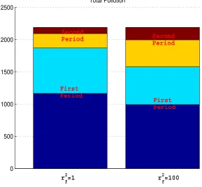
1) Generation under transmission and environmental constraints with preferences for pollution
in the second period:
We will examine whether the regulator can compute an equilibrium where there would be more production on weekends. We will set the weightsr2
1=100 andr 2
2=100 and keepr 1
f = 1, f = 1,2. The results obtained are visualized in figure 4.
In this figure, as in figure 2, the bars represent the total pollution levels corresponding to the transmission-&-environmental-constraint game with r2
f = 1 (first bar) and r
2
f = 100 (second bar). The two bottom fields together symbolise the first period’s pollution by firm 1 (bottom) and 2; the two top fields together represent the second period’s pollution by firm 2 (top) and 1. As expected, the pollution in the second period has increased. The pollution in period one has clearly diminished so has the contribution of firm 2 (“inefficient”). However, this equilibrium is achieved with higher prices (available in [4], omitted here) than before thus the consumers surplus is bound to diminish.
0 500 1000 1500 2000 2500
Total Pollution
r f 2
=1 r
f 2
=100
Second
Period Second
Period
First Period
[image:26.612.161.450.328.596.2]First Period
Fig. 4. Total pollution in 1000lb as a function of the weightsrt.
>1 attached to payoffs in the second period. This means that, because of r2
1=100 and r 2 2=100,
the firms perceive the marginal cost of violating the environmental constraint in period 2 as
λ2
E
100(βf + 2γfP
2
f), rather than as λ
1
E(βf + 2γfPf1) in the first period.
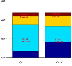
2) Generation under transmission and environmental constraints with preference for the first
firm:
We will examine whether the regulator can compute an equilibrium where there would be more production assigned to player 1 than it was in section V. We will set the weights r1
1 =r 2 1=100
for player 1 and keep r1 2 =r
2
2=1 for player 2.
1000 1500 2000 2500
Total Pollution
r 1 t
=100 r
1 t
=1
Second Period
Second Period
First Period
[image:27.612.158.450.273.542.2]First Period
Fig. 5. Total pollution in 1000lb as a function of the weightsrt.
VII. WHAT CAN THE REGULATOR LEARN FROM THE ABOVE RESULTS
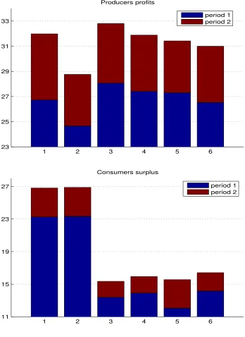
A. Implications for producer profits and consumer surplus
Figure 6 shows the plots of producer profits and consumer surplus (top and bottom respec-tively) as the constraints vary.
There are six bars in each of the panels of figure 6 for the cases as follows:
1) the base case,
2) generation subject to transmission constraints, 3) generation subject to emission constraints, 4) generation subject to both constraints,
5) generation subject to both constraints with preferences for pollution in the second period, 6) generation subject to both constraints with preference for the first firm.
We observe that the effect of a transmission constraint is negligible in terms of consumers surplus because prices and overall demands remain fairly stable. However, it diminishes producers profits as indicated by the second bar in the top panel of figure 6.
The introduction of an emission constraint introduces higher prices. This causes consumers surplus to substantially decrease and producers profits to increase. If both constraints are imposed simultaneously the emission limit effect surpasses that of the line limit by far so, this case is almost equivalent to the emission-limit-alone case.
1 2 3 4 5 6 23
25 27 29 31 33
Producers profits
period 1 period 2
1 2 3 4 5 6
11 15 19 23 27
Consumers surplus
[image:29.612.135.483.124.602.2]period 1 period 2
B. Results of varying the sharing rules
The results obtained for the case study indicate that the regulator can impact the producer profits and consumer surplus by imposing different levels of the responsibility for the joint con-straints’ satisfaction. In other words, varying the rules for how the burden of the environmental and transmission standards’ fulfilment is shared among the producers can generate a number of equilibria of uneven social desirability. The implication of this is that a (more) desired equilibrium can be chosen.
VIII. CONCLUDING REMARKS
We have proposed a methodology for the analysis of the impact of various constraints on electricity generation. In particular, this analysis should be useful for a regional government that is interested in an assessment of electricity supply changes due to an introduction of environmental constraints. For the case study considered in the paper, we notice the possibility of some market distortion when constraints become active.
We observe that introduction of an environmental constraint, which many businesses fear, may actually increase the business profits and make the consumers worse off economically.
We believe that thanks to our analysis, the regional government’s choices will be informed by the tradeoffs between constraint satisfaction, economic activity and electricity supply.
REFERENCES
[1] K.-C. Chu, M. Jamshidi, and R. Levitan,An approach to on-line power dispatch with ambient air pollution constraints,
IEEE Transactions on Automatic Control22(1977), no. 3, 385–396.
[2] J. Contreras, M. Klusch, and J. B. Krawczyk, Numerical solutions to Nash-Cournot equilibria in coupled constraint
electricity markets, IEEE Transactions on Power Systems19(2004), no. 1, 195–206.
[3] J. Contreras, J Krawczyk, and J. Zuccollo,Electricity market games with constraints on transmission capacity and emissions,
30th Conference of the International Association for Energy Economics, February 2007, Wellington, New Zealand.
[4] ,The invisible polluter: Can regulators save consumer surplus?, 13th International Symposium of the International
Society of Dynamic Games, June 30 - July 3 2008, Wrocław, Poland.
[5] A.G. Exp´osito and A. Abur,An´alisis y operaci´on de sistemas de energ´ıa el´ectrica, McGraw-Hill-Interamericana de Espa˜na,
2002.
[6] P. T. Harker, Generalized Nash games and quasivariational inequalities, European Journal of Operational Research 4
(1991), 81–94.
[8] A. Haurie and J. B. Krawczyk,Optimal charges on river effluent from lumped and distributed sources, Environmental
Modelling and Assessment2(1997), 177–199.
[9] ,An Introduction to Dynamic Games. Internet textbook, URL:
http://ecolu-info.unige.ch/˜ haurie/fame/textbook.pdf, 2002.
[10] B.F. Hobbs,Linear complementarity models of Nash-Cournot competition in bilateral and poolco power markets, IEEE
Transactions on Power Systems16(2001), no. 2, 194–202.
[11] B.F. Hobbs and J.-S. Pang, Nash-Cournot equilibria in electric power markets with piecewise linear demand functions
and joint constraints, Operations Research 55(2007), no. 1, 113–127.
[12] J.B. Krawczyk,Coupled constraint Nash equilibria in environmental games, Resource and Energy Economics27 (2005),
157–181.
[13] ,Numerical solutions to coupled-constraint (or generalised) Nash equilibrium problems, Computational
Manage-ment Science (Online Date: November 09, 2006), http://dx.doi.org/10.1007/s10287–006–0033–9.
[14] J.B. Krawczyk, J. Contreras, and J. Zuccollo,Thermal electricity generator’s competition with coupled constraints, Invited
paper presented at the International Conference on Modeling, Computation and Optimization (Indian Statistical Institute,
ed.), 9-10 January 2008, Delhi Centre, New Delhi, India.
[15] J.B. Krawczyk and S. Uryasev,Relaxation algorithms to find Nash equilibria with economic applications, Environmental
Modelling and Assessment5(2000), 63–73.
[16] J.B. Krawczyk and J. Zuccollo, NIRA-3:A MATLAB package for finding Nash equilibria in infinite games, Working
Paper, School of Economics and Finance, VUW, 2006.
[17] L. Mathiesen,A Cournot model with coupled constraints, The Norwegian School of Economics and Business
Administra-tion, Bergen, July 2007.
[18] E.A. Nurminski, Progress in nondifferentiable optimization, ch. Subgradient Method for Minimizing Weakly Convex
Functions and ǫ-Subgradient Methods of Convex Optimisation, pp. 97–123, International Institute for Applied Systems
Analysis, Laxenburg, Austria, 1982.
[19] J.-S. Pang and M. Fukushima,Quasi-variational inequalities, generalized Nash equilibria and multi-leader-follower games,
Computational Management Science1(2005), 21–56.
[20] R. Ramanathan,Emission constrained economic dispatch, IEEE Transactions on Power Systems9(1994), no. 4, 1994–2000.
[21] J.B. Rosen,Existence and uniqueness of equilibrium points for concave n-person games, Econometrica33(1965), no. 3,
520–534.
[22] W.D. Stevenson,Elements of power system analysis, McGraw-Hill New York, 1982.
[23] S. Uryasev and R.Y. Rubinstein,On relaxation algorithms in computation of noncooperative equilibria, IEEE Transactions
on Automatic Control39(1994), no. 6, 1263–1267.
[24] C. von Heusingen and A. Kanzow,Optimization reformulations of the generalized Nash equilibrium problem using
Nikaido-Isoda-type functions, Preprint 269, University of W¨urzburg, Institute of Mathematics, 2006.
[25] J.-Y Wei and Y. Y. Smeers,Spatial oligopolistic electricity models with Cournot generators and regulated transmission