Munich Personal RePEc Archive
Productivity Differences in an
Interdependent World
Fadinger, Harald
ECARES, Unversité Libre de Bruxelles, Universitat Pompeu Fabra
March 2008
Productivity Differences in an Interdependent World
Harald Fadinger
∗ECARES & Universitat Pompeu Fabra
January 2008
Abstract
This paper studies cross country differences in productivity from an open economy perspective by using
a Helpman-Krugman-Heckscher-Ohlin model. This allows to combine tools from development accounting
and the trade literature. When simultaneously fitting data on income, factor prices and the factor content
of trade, I find that rich countries have far higher productivities of human capital than poor ones, while
differences in physical capital productivity are not sytematically related to income per worker. I estimate an
aggregate elasticity of substitution between human and physical capital that is significantly below one, clearly
rejecting a world that consists of a collection of Cobb-Douglas economies and also one where Heckscher-Ohlin
trade is important.
Keywords: Heckscher-Ohlin, Productivity Differences, Development Accounting, Open Economy Growth.
JEL classification codes: F11, F43, O11, O41, O47.
∗An earlier version of this paper was circulated under the title ”Development Accounting in a Heckscher-Ohlin-World”. I thank
my advisor Jaume Ventura for encouraging me to work on this topic and for many insightful discussions. I am especially indebted
to Antonio Ciccone and Gino Gancia for many helpful discussions and I would also like to thank Fernando Broner, Paula Bustos,
Chiara Forlati, Alberto Mart´ın, Michael Reiter, Thijs van Rens, Maurizio Zanardi as well as participants in seminars at Universitat
Pompeu Fabra, ECARES, Universitat de Barcelona and in the Minerva-DEGIT XI conference, the 2006 annual conference of
the European Trade Study Group, the 2007 RES annual conference and the 2007 SED annual meeting for their comments and
suggestions. Financial support by the Austrian Academy of Science under a DOC scholarship is gratefully acknowledged. The
author is also member of ECORE, the recently created association between CORE and ECARES. Correspondence: ECARES,
1
Introduction
Finding answers to the question why some countries are so much richer than others is one of the fundamental
challenges in economics. While according to the consensus view cross country differences in factor endowments
and differences in productivity are more or less equally important causes for the cross country variation in income
per worker (Caselli (2005)), there is little evidence whether individual economies are actually well described by
an aggregate Cobb-Douglas production function and whether differences in productivity across countries are really factor neutral as usually assumed in the quantitative growth literature.
Moreover, even though trade is empirically very important 1 and may also potentially affect the shape of
countries’ aggregate production possibility frontiers (Ventura (2005)) most research in growth and development
still uses closed economy models when estimating cross country differences in productivity. This may not only
be too restrictive for theoretical reasons but - since these models have by their very nature nothing to say about
trade - it also leaves one of the best sources of cross country information - bilateral trade data - completely
unexploited.
A second, independent line of investigation in international trade deals with the prediction of the
Heckscher-Ohlin-Vanek (HOV) Theorem, that states that capital abundant countries should export capital (through trade
in goods), while labor abundant countries should export labor. This research, which uses trade data to evaluate the validity of this theory, finds that cross country differences in productivity greatly help to explain factor flows
embodied in trade.
The goal of this paper is to merge these two approaches by using a world equilibrium model - the
Helpman-Krugman-Heckscher-Ohlin (1985) model - to estimate factor augmenting productivities, thereby providing a
unified framework and exploiting the information contained both in income and in trade data. This model has
been the workhorse of trade economists for more than two decades.2 It combines inter-industry Heckscher-Ohlin
trade with intra-industry trade due to increasing returns and love for variety. I augment the model for differences
in the efficiencies with which factors are used across countries to introduce a potential role for productivity in
generating cross country variation in income per worker.
The model encompasses two very popular views of the world as particular cases. The first one is the neoclassical one sector model with factor deepening that is the standard framework in the quantitative growth
literature, while the second one is the Heckscher-Ohlin model with conditional factor price equalization, the
canonical model for estimating productivities in the trade literature (Trefler (1993,1995)). Cases of intermediate
integration are described by a world that separates into multiple cones of diversification, with different sets of
countries specializing in the production of different sets of goods.
I simultaneously fit data on income, endowments, factor prices and the factor content of trade. This provides
me with over-identifying restrictions that enable me to calibrate productivities and at the same time allow me
1
In the early 1990ies trade already amounted to 38 per cent of world income and by the turn of the millennium it had reached
52 per cent of world output (Trade is measured as exports+imports, data are from the Penn World Tables 6.1.).
2
While the original formulation of the model is due to Helpman (1981), Helpman and Krugman (1985) dedicate an entire book
to evaluate the fit of the model and to estimate the values of underlying parameters. More specifically, I test
the factor deepening case against cases with multiple cones of diversification and ones where conditional factor
price equalization occurs and I estimate the elasticity of substitution between human and physical capital.
My main findings are that the factor deepening model with factor specific productivities and weak
comple-mentarity between human and physical capital vastly outperforms the other versions of the model considered
in this paper. In particular, the elasticity of substitution between human and physical capital is estimated to
be significantly lower than one, so that the Cobb-Douglas model is clearly rejected. Rich countries have far
higher productivities of human capital than poor ones, while there is no clear relation between physical capital productivity and income per worker. Moreover, my results imply that the model best supported by the HOV
Theorem has no Heckscher-Ohlin motiv for the exchange of goods and all trade is due to increasing returns and
love for variety.
In terms of intellectual ancestors, this paper integrates two lines of investigation. The first one is the literature
on development accounting, which uses income and endowment data to measure productivity differences. Some
of the classical contributions are due to King and Levine (1994), Klenow and Rodriguez-Clare (1997), Prescott
(1998) and Hall and Jones (1999). See Caselli (2005) for a survey. A stable result of these studies is that total
factor productivity is strongly positively correlated with income per worker and accounts for at least half of
the cross country variation of this variable. Caselli (2005) adds factor specific technology differences to this
approach and discovers that rich countries have higher productivities of human capital than poor ones, whereas poor countries have higher productivities of physical capital than rich nations.
The second strand of research, that uses trade data to measure productivity differences, is the literature that
tests the prediction of the Heckscher-Ohlin-Vanek (HOV) equations. They state that countries’ trade structure
is such that they are net exporters of the services of those factors, in which they are more abundant than the
world average. A seminal contribution by Trefler (1993) shows how the HOV equations can be used to solve
for the unknown factor specific productivities of each country that equalize measured and predicted factor flows
under the assumption that differences in factor prices across countries are caused exclusively by variation in
factor productivities. He finds that rich countries have both higher productivities of labor and physical capital
than poor countries.
In another important paper Davis and Weinstein (2001) relax the assumption that differences in factor prices are caused only by differences in productivities. They show that both Hicks-neutral differences in total factor
productivity, which they estimate using input-output data, and local factor abundance must be taken into
account in order to improve the fit of the HOV equations. However, their sample is limited to ten large OECD
countries, so that they have nothing to say about productivity differences between rich and poor countries.
This paper goes beyond the previous contributions because I allow both for factor productivities and local
factor abundance to matter for income differences and I match data on income, factor prices and trade at
the same time. Also, since I put more structure on the underlying model, I am able to estimate the value of
underlying parameters and to test different special cases of the model.
of studies, summarized by Hamermesh (1986), have attempted to estimate this parameter at various levels of
aggregation and using both cross section and time series data. Despite of this, the evidence on its value remains
inconclusive, which may potentially reflect mis-specification because this body of research considers exclusively
Hicks neutral technological change. Recently, Antr`as (2004) discusses the bias that arises from this restriction
and estimates the elasticity of substitution between capital and labor for the US economy allowing for factor
augmenting productivity differences using time series data. In line with my results, most of his estimates are
significantly lower than one.
Finally, Waugh (2007) performs a development accounting exercise in an open economy framework that extends Eaton and Kortum (2002). However, he restricts his analysis to Cobb-Douglas production technology
and his main interest is to investigate the role of trade in accounting for cross country income differences.
Summing up, the main contributions of this paper are threefold: Firstly, it integrates development accounting
with trade theory and methods. Secondly, the paper proposes to introduce formal over-identification using data
from outside the model to evaluate the fit of the productivity calibrations. Thirdly, this buys me a very precise
estimate of the elasticity of substitution between human and physical capital, a clear rejection of the aggregate
production function being Cobb-Douglas and the possibility to test which model performs best in terms of
fitting the HOV equations.
The outline of the paper is as follows: In the next section I develop a theoretical model of the world
economy with trade due to factor proportions and love for variety that includes factor specific cross country productivity differentials. In section three I show how factor productivities can be recovered from the model
when data on countries’ endowments and factor prices are fed in and I discuss how the HOV equations can be
used in this framework to evaluate the plausibility of the calibrated productivities and to estimate the values
of underlying parameters. In section four I present the results of calibrating productivities in the
Helpman-Krugman-Heckscher-Ohlin framework and use the calibrated productivities to perform a development accounting
exercise. The last section concludes.
2
The Helpman-Krugman-Heckscher-Ohlin Model
2.1
Assumptions and Setup
The model presented in this section is a standard model of international trade. There are two reasons for trade
in this environment. The first one is due to increasing returns. Consumers value variety and each variety is produced by a monopolist because increasing returns are internal to the firm and new varieties can be invented
without cost. Since consumers want to consume all varieties each producer serves the world market for her
particular variety, which leads to trade within sectors. The second motive for trade is factor proportions. There
exist many sectors each of which uses factor inputs with distinct intensities and countries differ in the ratios of
their endowments. This gives rise to Heckscher-Ohlin trade and countries produce on average more varieties in
those sectors that use its relatively abundant factor intensively. I also introduce cross country differences in the
leads to a different amount of production, depending on the country where production is performed.
The Heckscher-Ohlin part of the model adds two main effects to the standard model used in the
develop-ment accounting literature. The first one is structural change, that is the possibility for countries to adapt their
production structure to their factor endowments. Countries which are abundant in physical capital will
concen-trate their production in sectors that are intensive in this factor. This tends to increase the role of variation
in factor endowments in explaining cross country income differences because countries can employ their factors
more efficiently. The other one is terms of trade. These work exactly in the opposite direction because they
depress the income of those countries that produce goods which are intensive in the globally abundant factor, thereby reducing the importance of factor endowments in accounting for income differentials. The monopolistic
competition part is introduced mainly to explain trade in the absence of differences in factor proportions, as
is the case in the standard model for development accounting, but it has no important impact on countries’
aggregate production possibility frontiers.
The flexible benchmark model of the world economy relies on the following main assumptions.
A.1: Countries are open to trade in goods and possess perfectly competitive factor markets.
A.2: Goods markets are monopolistically competitive.
A.3: Factors are immobile between countries and perfectly mobile within countries.3
A.4: Each country is endowed with human capitalHc and physical capitalKc.4
A.5: Productivity is specific to a factor located in a country.
A.6: Each country has access to technologies to produce inIsectors, that vary in their capital intensities.
A.7: Consumers in all countries have identical, homothetic preferences with fixed expenditure shares. 5
The model is then easily described by Assumptions A.1-A.7 and the specification of demand and supply.
3
The immobility of labor is probably not a very controversial assumption. Even though some mobility of people can be observed,
there exist very large barriers to migration from poor to rich countries. Starting at least with Lucas (1990) a large literature in
International Economics has been dealing with the question why capital does not flow from rich to poor countries. Caselli (2006)
makes the interesting point that capital may actually be distributed quite efficiently across countries, so that there is no reason to
observe large capital flows from rich to poor nations.
4
Following the growth literature the factor ”human capital” is measured as labor endowments in efficiency units, which is
different from the convention used in the trade literature, where human capital is usually the amount of skilled labor. Because the
model has only two factors this seems to be the adequate way to measure labor endowments.
5
2.2
Demand
Consider a world economy with countries indexed byc∈C and sectors indexed byi∈I.6 Assuming that trade
is balanced, aggregate expenditure of countrycequals its aggregate income.
Ec =PcYc= I
X
i=1 Eic=
I
X
i=1
βiEc, (1)
where PcYc is GDP of country c in dollars, and Yc is GDP in purchasing power parities and is measured in
aggregate consumption units. Aggregate spending is split acrossI sectors with fixed expenditure sharesβi.7
The ideal aggregate price index is Cobb-Douglas. It measures the minimum expenditure to buy one unit of
the aggregate bundle of goods.
Pc = I
Y
i=1
Pi
βi
βi
, (2)
wherePi are the sectoral price indices.
Sectoral price indices are constant elasticity of substitution composites of the prices of sector specific varieties.
Pi =
Z Ni 0
pi(n)1−σdn
!1−1σ
, (3)
where σ >1 is the elasticity of substitution between any two varieties andNi =PCc=1Nicis the total number of varieties produced in sector i.
The form of the sectoral price indices implies that there is love for variety and aggregate consumption is
increasing in the number of varieties available in each sector.
The demand function of countrycfor varietynproduced in countryc′in sectoriimplied by the price indices can be found from the sectoral price index by using Roy’s law.
xicc′(n) =
pi(n)−σ
Pi1−σ βiEc (4)
2.3
Behavior of Firms and Technology
Final goods are freely traded and are produced by monopolistically competitive firms.
In each sector firms choose a variety and an optimal pricing decision taking as given the decisions of the
other firms in the industry.8 The output of an industry consists of a number of varieties that are imperfect
substitutes for each other. Production of each variety is monopolistic because of economies of scale. In the
model the invention of a new variety is costless, so firms always prefer to invent a new differentiated variety
instead of entering in price competition with an existing firm.
In each country firms are homogeneous within a sector. Firms’ technologies differ across sectors by the capital intensity of production for given wages, wc, and rental rates, rc. Varieties of final goods are produced
6
I slightly abuse notation by denoting withCandIboth the sets of countries and goods and their cardinalities.
7
A possible interpretation for this setup is that each country has an aggregate Cobb-Douglas production function that produces
a final good which can be used for consumption and investment.
8
using both human capital Hic(n) and physical capital Kic(n) with constant marginal cost and a fixed cost,
f. Production technology, represented by the homothetic total cost function T C (5), is CES in each sector9
and varies across countries because of differences in factor productivities. Productivities are specific to factors
located in country c, so that a country’s productivity is described by the duple {AKc, AHc}, which are the
productivity of physical capital and human capital in countryc.
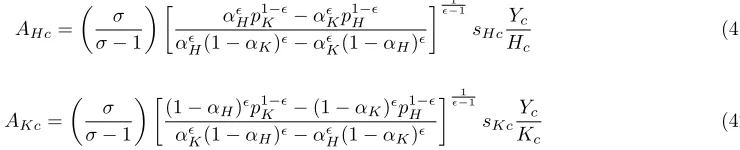
T C(qic) =
"
αǫ i
r
c
AKc
1−ǫ
+ (1−αi)ǫ
w
c
AHc
1−ǫ#
1 1−ǫ
(f+qic), (5)
where αi ∈ [0,1] is the physical capital intensity of sector i and ǫ ∈ [0,∞) is the elasticity of substitution
between human capital and capital.
Monopolistic producers in sectoriof countrycmaximize profits subject to the demand function
xic′ =
p−σi Pi1−σβi
C
X
c=1
Ec. (6)
Optimality implies that marginal revenue equals marginal cost. Note that given this constant elasticity demand
function the solution to the firms’ profit maximization problem implies that the price charged by a firm in sector
iin countrycis a constant markup over its marginal cost as long as firms are active in that sector in countryc.
pi =
σ σ−1
"
αǫ i
r
c
AKc
1−ǫ
+ (1−αi)ǫ
w
c
AHc
1−ǫ#
1 1−ǫ
(7)
If a sector is located in a country, free entry of firms drives profits to zero, so that firms price at their average
cost. This determines the number of firms in each sector endogenously.
[αǫirˆ1c−ǫ+ (1−αi)ǫwˆ1c−ǫ]
1 1−ǫ
f qic
+ 1
≥pi (8)
The combination of the pricing rule, the free entry condition and the form of the fixed cost imply that firms’ optimal output is the same in all sectors and countries (as long as it is positive).
q∗= (σ−1)f (9)
2.4
Equilibrium
It turns out to be useful to rewrite the model in terms of variables in efficiency units. Following Daniel Trefler
(1993), let me define ˆHc≡AHcHc, ˆKc ≡AKcKc, ˆwc≡ AwHcc and ˆrc≡ ArKcc .
These are factor endowments in efficiency units and efficiency adjusted factor prices. So, for example, one
unit of efficient physical capital is equivalent to AKc units of plain physical capital, and one unit of efficient
physical capital, which is measured in common units across countries, costs AK,c1 as much as one unit of plain
physical capital, that may differ in efficiency across countries. Hence, capital prices in countryc may be higher
9
The assumption that elasticities of substitution are the same across sectors rules out factor intensity reversals - the possibility
that a sectoriis more intensive in physical capital than sectori′for some combination of factor prices and more intensive in human
than in countryc′ because buying one unit of capital in countryc provides ownership of more efficient units of
capital or because capital is scarcer in countryc.
With this redefinition of variables I am able to describe the world economy as an ordinary
Helpman-Krugman-Heckscher-Ohlin (1985) model without productivity differences in which factor endowments in each country are
measured in efficiency units, while leaving the structure of the model formally equivalent to the one described
by the production possibilities and demand structure listed above. The advantage of this formulation is that
the extensive theory available on the factor proportions theory and its monopolistic competition hybrid, as
discussed in Helpman and Krugman (1985), can be directly applied to this model.
In general, it may not be profitable to produce varieties in all sectors in every country because production
in sectors that use the locally scarce factors intensively may be unprofitable. In this case, countries will be
located in different cones of diversification. A cone of diversification is a set of countries that produce at least in
two common sectors. Those countries have common efficient factor prices, and when the number sectors active
in the cone is larger than the number of factors, individual countries’ production of varieties is undetermined
and only the aggregate number of varieties produced in each sector in the cone is unique. Consequently, let
d be a set of countries with common efficient factor prices. Given this, one can define an equilibrium of the
Helpman-Krugman-Heckscher-Ohlin model.
Definition 1: AnEquilibrium is a collection of goods prices{pi}, efficiency adjusted wages{wˆd}, efficiency adjusted rental rates{rˆd}, and numbers of sectoral varieties{Nid}such that firms maximize profits, expenditure
is minimized, factors are fully employed and goods markets clear in every set of countriesd.
Since the general model is rather complex, let us instead take a look at some representative examples to
learn something about the forces that determine countries’ relative incomes in this world. The intuition gained
in these specific cases will carry over to the general model.
Example 1: Factor Deepening
A.8 All sectors have identical factor intensities (αi=αfor alli∈I).
This assumption eliminates both the role of structural change and terms of trade effects. From the pricing
conditions (7) we have that goods in all sectors have the same price pi =pi′ =pand countries produce some
varieties in all sectors. Taking this into account, it is not difficult to solve for the aggregate production function
implicit in this model10
Yc=p
σ
σ−1
[α(AKcKc)
ǫ−1
ǫ + (1−α)(AHcHc) ǫ−1
ǫ ] ǫ
ǫ−1, (10)
where
p= ( I
Y
i=1
(Ni
βi
)βi)σ1−1. (11)
10
To get this note that all prices are the same, and divide the factor market clearing conditions, which by Shephard’s Lemma
-can be obtained by partially differentiating (5) with respect to factor prices, to solve for the wage/rental, wˆc
ˆ
rc = (
1−α α )(
AKcKc
AHcHc)
1 ǫ.
It can be seen from (10) that countries’ aggregate production function is CES with an elasticity of substitution
between physical and human capital equal to ǫ. This is the world with factor specific productivities described
by Francesco Caselli (2005) in the Handbook of Economic Growth. The main features of this world are that
countries experience decreasing returns to factor accumulation and that terms of trade do not matter for
aggregate income because all relative goods prices are one. There is an aggregate scale effect due to love for
variety, but it is irrelevant for relative incomes because all varieties are available in all countries.
In this world all trade is due to love for variety, as producers export their variety to all other countries.
Imports by country c′ of variety n produced in sector i in country c are a fraction of production that is proportional to the size of the importing country.11
xcc′i(n) =
p−σ i
Pi1−σσiEc= Yc
PC
c=1Yc
qci(n) (12)
Even though differences in factor endowments across countries do not constitute a reason for trade in this world, goods trade embodies factors, since countries that are abundant in efficient physical capital produce
vari-eties much more capital intensively than efficient human capital abundant ones and therefore are net exporters
of this factor.
An additional assumption leads us back to the Cobb-Douglas world, that has been the focus of the analysis
in most of the development accounting literature.12
A.9: ǫ= 1
Then the aggregate production function is Cobb-Douglas.
Yc =p
σ σ−1
AαKcA1Hc−αK α
cHc1−α=p
σ σ−1
AcKcαHc1−α, (13)
where I have defined Ac ≡AαKcA
1−α
Hc . This view point of the world economy is similar to Caselli’s, just that with a unit elasticity of substitution, only total factor productivity is identified. Countries experience decreasing
returns and terms of trade effects are absent.
Example 2: Conditional Factor Price Equalization (CFPE)
A completely different picture of the world arises if we drop assumptionsA.8andA.9, and instead maximize
the role of structural change. We do this by assuming that trade integration is so strong, that trade in goods
is able to make up for the immobility of efficient factors.
A.10: Conditional on measuring endowments in efficiency units factor prices are equalized in the world economy.
In this extreme case the equilibrium of the world economy is akin to the one of a hypothetical world, in which
all impediments to movements of factors measured in efficiency units have been abolished. Call this equilibrium
11
This follows from the definition of the sectoral price index and the fact thatPCc=1piNicqic=βi
PC c=1Yc 12
the integrated equilibrium. The Factor Price Equalization Set is the set of distributions of efficient factor
endowments across countries, such that the world economy is able to replicate the integrated equilibrium.13
This implies that the world economy has the allocations of the integrated equilibrium if every country can fully
employ its resources when using the same capital to human capital ratios in each sector as in the integrated
equilibrium given its endowments of efficient human and physical capital. The size of this set is larger if
different sectors use very different capital to human capital ratios for given factor prices (αi varies a lot across
sectors) because even countries with extremely unbalanced factor endowments will be able to find production
patterns such that they can employ their factors using the integrated equilibrium techniques. Still, in this world, marginal products of physical units of capital and human capital are not equalized across countries because of
differences in factor productivities. Consequently, disparities in factor prices stem only from differences in factor
productivities and not from variation in the abundance of human capital and physical capital across countries.
Assume that sectoral input ratios are sufficiently extreme and expenditure on sectors with extreme factor
proportions is large enough in order for conditional factor price equalization to hold for the world economy, i.e.
ˆ
wc = ˆwc′ = ˆw and ˆrc = ˆrc′ = ˆr for all c ∈C. Then - as discussed - it is sufficient to analyze the equilibrium
of the integrated economy. For analytical tractability let ǫ → 1 so that sectoral production functions are
Cobb-Douglas. In this case one can show that the aggregate production function of the world economy is also
Cobb-Douglas.14
Qw=BKˆ
P
i∈Iαiβi
w Hˆ
(1−Pi∈Iαiβi)
w , (14)
where
B≡( I
Y
i=1
Ni
βi )βi
σσ−1 I
Y
i=1
"
(1−αi)βi
PI
i=1(1−αi)βi
#(1−αiβi)"
αiβi
PI
i=1αiβi
#αiβi
(15)
and
ˆ
Hw= C
X
c=1
ˆ
Hc, Kˆw= C
X
c=1
ˆ
Kc. (16)
There are decreasing returns to factor accumulation in efficiency units at the world level. World factor prices
are given by
ˆ
w= (1−X
i∈I
αiβi)B ˆ
Kw ˆ
Hw
!Pi∈Iαiβi
(17)
and
ˆ
r= (X i∈I
αiβi)B ˆ
Hw ˆ
Kw
!(1−P
i∈Iαiβi)
. (18)
13
For a thorough discussion of these concepts see, for example, Helpman and Krugman (1985).
14
To obtain this, solve for sectoral factor shares and total factor shares and divide these equations to obtain sectoral factor use
in terms of aggregate factor endowments. Then use the market clearing conditions to solve for goods prices and substitute them in
the definition of the price indices to get the implicit aggregate production function of the world economy. Finally, use the definition
of sectoral production functions, defineQic=Nicqicand substitute the sectoral factor use in terms of aggregate endowments to
Consequently, factor prices are determined at the world level and not at the country level. Income of countryc
is given by
Yc =AHcHcwˆ+AKcKcr.ˆ (19)
To the extent that factor prices are given for individual countries, countries’ aggregate production functions are linear and countries experience constant returns to factor accumulation. The infinite elasticity of
substi-tution between factors reflects structural change. Countries absorb additional units of factor endowments by
changing their production structure while holding constant sectoral production techniques, instead of using
factor deepening like in Example 1 or in the closed economy.
In this world there is both intra-industry trade (because of love for variety and monopolistic competition)
and inter-industry trade (because of differences in factor endowments across countries). Countries that are more
abundant in an efficient factor than the average of the world economy are net exporters of this factor. Even
though all countries produce in all sectors, it is not necessarily true that countries produce more in those sectors
that use their abundant factor intensively because individual countries’ production patterns are undetermined,
when the number of sectors is larger than the number of factors,.
We have now seen two very diverse views of how countries’ aggregate production possibilities may look like.
In general, however, the world is likely to be somewhere between the two extremes of the Factor Deepening world
and Conditional Factor Price Equalization and will combine features of both. If differences in efficient factor
endowments are too large, efficient factor prices cannot be equalized in the whole world. Instead, there will be
multiple cones of diversification. Between those cones, there will generically exist countries that specialize in
the production of varieties in a single sector.
Example 3: Multiple Cones
Assume there are only two sectors,i∈ {H, K} withαK > αH. Since it is not possible to solve this model
analytically, let us take goods prices as parameters. With only two sectors, sectoral production patterns are
determined in each country. Countries with extremely high efficient physical to human capital ratios specialize
in producing varieties in the K-sector. Countries with intermediate factor endowment ratios have diversified
production structures and produce varieties in both sectors, while countries with very low efficient physical to
human capital ratios specialize in the H-sector.
It is easy to show that for countries outside the cone of diversification the aggregate production function has
the form of the sectoral production function of the sector in which they specialize. 15
Yc=pi
σ
σ−1[αi(AKcKc)
ǫ−1
ǫ + (1−αi)(A
HcHc)
ǫ−1
ǫ ]ǫ−ǫ1 (20)
In this case countries experience decreasing returns and the elasticity of substitution isǫbecause additional
units of factors are absorbed by factor deepening. Terms of trade effects push up the income of countries that specialize in the sector which has a high relative price. Countries that lie in the cone of diversification, on the
15
Divide the factor market clearing conditions to get the wage/rental and use this equation together with the pricing equation
other hand, have linear production technologies, reflecting again the fact that they are capable of absorbing
additional units of factors through structural transformation.
Yc= ˆwdAHcHc+ ˆrdAKcKc (21)
where
ˆ
wd=
σ σ−1
αǫ
Hp1K−ǫ−αǫKp1H−ǫ
αǫ
H(1−αK)ǫ−αǫK(1−αH)ǫ
1−1ǫ
(22)
ˆ
rd=
σ σ−1
(1−αH)ǫp1−ǫ
K −(1−αK)ǫp
1−ǫ H
αǫ
K(1−αH)ǫ−αǫH(1−αK)ǫ
1−1ǫ
(23)
Factor prices are functions of goods prices only and consequently depend on the endowments of the world
economy.16 From the formulas (22) and (23) one can see that an increase in the price of a sector’s output leads
to a more than proportionate rise in the price of the factor that is used intensively in that sector. This is the
Stolper-Samuelson effect. The intuition is that an increase in an industry’s price shifts production towards that
sector and thereby increases relative demand for the intensively used factor. Whether an increase in a sectoral
price decreases or increases aggregate income depends on how much a country is producing in each sector (which
in turn depends on its endowments).
This example provides all the mechanism present in the general model. The world sorts into cones of
diversification between which lie countries that specialize in specific sectors. As a consequence the mapping
between endowments, factor prices, income and productivity changes its shape depending on whether a country is located in a cone or specialized. Having discussed the properties of the model, let us now turn to calibrating
productivities in this world.
3
A Method for Productivity Calibration
Given measures of factor productivities for every country I could test if the models described in the previous
section are a reasonable representation of the real world. Unfortunately, I lack exactly these measures of
productivities. Instead, in a first step I will follow the convention of the development accounting approach to
assume that the model is specified correctly, and back out productivities from the model given some additional
information about other endogenous variables. Subsequently, I will test the model fit using trade data.
The procedure is to use information on endowments {Hc}, {Kc}, wages, {wc}, and rental rates, {rc}, in
order to back out the 2C unknowns{AKc}, {AHc} from the equilibrium conditions of the model. This allows
me to fit perfectly the cross section of income {Yc} and labor and capital income shares, {sHc} and {sKc},
respectively, taken as given a combination of sectoral factor intensities {αi}, expenditure shares {βi} and an
elasticity of substitution ǫ.
16
To derive this use the pricing conditions for the relevant goods and solve for factor prices in terms of goods prices. These
This method for calibrating productivities is analogous to the usual calibration exercise performed in the
development accounting literature. The main complication is that productivities have to be determined
simul-taneously with the unknown specialization patterns, equilibrium prices and production levels in each country,
because the relationship between a countries’ inputs and outputs generally depends on endowments and the
demand structure of the whole world economy. More formally, a Productivity Calibration Problem is
defined as follows.
Definition 2: A Productivity Calibration Problem(PCP) is a collection of goods prices{pi}, efficiency adjusted wages {wˆd}, efficiency adjusted rental rates {rˆd}, numbers of sectoral varieties {Nid} and factor
productivities {AHc}, {AKc} such that given a cross section of human capital endowments {Hc}, physical
capital endowments {Kc}, wages {wc}, rentals {rc} and parameters {αi}, {βi}, ǫ, σ and f, firms maximize
profits, expenditure is minimized, factors are fully employed and goods markets clear for alld17.
One can show that a solution toPCPis also anEquilibriumgiven efficient factor endowments, and that for
given efficient factor endowments anEquilibrium also solves thePCPand measured productivity differences
are zero, which is obviously necessary for the concept of PCPto make sense.
Solving thePCPrequires the use of numerical methods. There are three main challenges. First, the large
number of countries in the sample (96), which I use to have a representative picture of the world economy. Second, the fact that one cannot apply standard methods for computing equilibria because parameters and
variables have been exchanged (since {AHc},{AKc} are unknown). Third, that I allow countries to specialize
into multiple cones, which makes computation much more complex because corner solutions might occur.
I compute a solution to thePCPby imposing a specialization pattern, solving the resulting nonlinear system
of equations and checking if the solution satisfies the non-negativity restrictions imposed on the variables. If
it does, I accept the solution, otherwise I guess another specialization pattern until a solution is found. For
reasons of computational tractability I restrict my attention to models with two sectors.18
As a next step I would like to find reasonable parameter values for production and demand {αi}, {βi} ǫ,
for which to solve the model because results will be sensitive to the choice of these parameters19. In addition, I
would like to test if certain restrictions imposed on the parameters by standard models, likeαi=αorǫ= 1 or
AHC =AKC are realistic.
3.1
Using Trade Data to Evaluate the Model
To estimate these parameters I use the model’s prediction on trade. The testable hypothesis of the
Heckscher-Ohlin-Vanek (HOV) equations is that a country should export (through trade in goods) the services of those
(efficient) factors with which it is abundantly endowed relative to the world average and import its relatively
17
An exact mathematical definition of thePCPcan be found in the appendix.
18
As discussed in the appendix, the solution toPCPis unique under some restrictions.
19
In the simulations I setσf= 1 and define ˜pi≡σ−1
σ pifor convenience, since the productivities generated by thePCPdo not
scarce factors. The predictions on factor trade provide over-identifying restrictions that enable me to find the
combination of parameter values that best match moments of the data and at the same time allow me to test,
if certain constraints on parameters are valid.
The HOV-equations hold for a class of trade models that satisfy a consumption similarity condition (see
Trefler and Zhu (2005)) and perfect competition in factor markets. In particular, they apply to the
Helpman-Krugman-Heckscher-Ohlin model, and all its versions considered in this paper.20
Because the HOV-equations are a statement about factor flows embodied in trade and not directly about
trade in goods, one needs to define the factor content of trade. Let f ∈ {H, K} denote factors, Vf c denote endowments of factor f in country c, i= 1, ..., I denote goods and let Dc be the F ×I factor use matrix in
countryc, with elementsbf icdenoting the use of factorf in the production of one unit of goodiin countrycand
rowsDf c, that state the use of factorf per unit of output in each sector. Let Bc be country c’s input-output
matrix and denote factor prices byπc = (wc, rc). Then, for example, the direct use of human capital measured
in efficiency units in the production of one unit of goodiin country cin the above models is
dHic=
σ σ−1p
ǫ
iw−ǫc (1−αi)ǫAǫHc. (24)
In addition, thefth row of the direct factor use matrix of the United States in efficiency units is
Df U S=π−ǫU SAǫf U SDf, (25)
where Df is common to all countries because of free and costless trade and the absence of industry specific
(Ricardian) technology differences across countries. The factor use matrix measured in efficiency units of every
countryccan be expressed as a function of the one of the US,
Df c=πc−ǫDfAǫf c=
πU S
πc
ǫ
Af c
Af U S
ǫ
Df U S. (26)
Following Trefler and Zhu (2006), in the presence of trade in intermediate goods, the measured factor content
of trade in efficient factorf by countryc is defined as
Ff c∗ =Ef cXc−
X
c′6=
c
Ef c′Mcc′, (27)
whereEf c is an 1×I vector that converts trade in goods into trade in factors measured in efficiency units,
Xcis anI×1 vector of countryc’s exports andMcc′ areI×1 vectors of bilateral imports of goods by country
c from country c′. The total net efficient factor content of country c’s trade is computed as the amount of
efficient factorf embodied in countryc’s exports,Ef cXc, minus the quantity of efficient factorf that country
cimports from other countries,P
c′6=cEf c′Mcc′. Here,Ef c is thec’th column ofEf= ˜Df(I−B)−1, which is a
complicated function of the efficient factor use matrices Df c, and the input-output matricesBc of all countries
in the world. 21
20
Interestingly, they apply to the Heckscher-Ohlin model with perfect competition only in special cases. One is (conditional)
factor price equalization, and the other one is complete specialization of all countries, a borderline case. The fact that many models
imply the HOV equations means also that one cannot use them to test a particular trade model against an alternative, unless one
has an underlying structural model that generates testable data.
21
The reason why one needs to consider the input-output relations of the whole world to compute the factor
content of a single country’s trade is trade in intermediate goods. For example, if the US imports cars from
Germany that have been produced using Chinese steel, the factors embodied in the Chinese steel must be
evaluated using the Chinese factor use matrix, and not the German one.
To obtain the HOV equations in efficiency units, one needs to make the assumption that each countryc
consumes a fraction of the world’s total consumption of all goods produced in a countryc′which is proportional
to the importing country’s size.
A.11: Ccc′ =scP
c′∈CCc′
This condition is met by the class of models considered in this paper, since - because of love for variety and
monopolistic competition - each country imports a fraction of every good produced in each country and the
entire production of every good is consumed.
As Trefler and Zhu (2005) showA.11is sufficient (and in general also necessary) for the HOV-equations to
hold in efficiency units. Hence, we have that
Ff c∗ =Af cVf c−sc
X
c∈C
Af cVf c= ˆVf c−scVˆf w. (28)
Equation (28) states thatF∗
f c, the measured efficient factor content of trade, equals the difference between a country’s endowments of factor f in efficiency units, ˆVf c and the world endowments of this factor in efficiency
units, ˆVf w, multiplied by country c’s share in world GDP. The right hand side of (28) is usually called the
predicted factor content of trade.
Consequently, a country exports an efficient factor f in net terms (i.e. F∗
f c > 0) whenever ˆVf c > scVˆf w because it consumes a fraction of the world efficient endowments that is proportional to its size.
Let us now turn back to the question how to determine the parameter values of thePCP. As we noted, the
HOV-equations provide restrictions on the factor productivities computed from the model for given parameter
valuesθ = ({αi},{βi}, ǫ). LetFf c∗(θ) be the factor content of trade constructed using the factor use matrices
that have been generated by the model, Df c(θ). Dividing (28) by the equation for the US and normalizing
Af U S to one, we obtain the following relation.
Af c(θ) = Yc
YU S
Vf U S
Vf c +F
∗ f c(θ)
Vf c
− Yc
YU S
F∗ f U S(θ)
Vf U S
+uf c, (29)
where I have augmented the equation for an i.i.d error term, uf c. Hence, a country has a high factor
productivity relative to the US if its relative factor-output-ratio is low and if it exports more of a factor relative
to its endowments compared to the US controlling for its relative size. If{Af c(θ)}are good estimates of factor
productivities, equation (29) should hold roughly with equality.
This test requires - in addition to calibrated values of Af c(θ) - information on countries’ input-output
matrices, on bilateral trade at the sector level and on the factor use matrix of the US (or any other reference
To make this more formal, I use a GMM estimation procedure to choose the vector of parametersθ.
I use the following L=4 orthogonality conditions to estimate θ: E(uf c) = 0 and E(uf cYYU Sc ) = 0 for f ∈
{H, K}. These conditions exactly identify θ in the two sector multiple cone case and over-identify it in the
factor deepening and the CFPE case.
LetZ= [1, Y
YU S] be the matrix of instruments, letgc(θ) =Z
′
cuc(θ) and letg(θ) = 1/C
PC
c=1gc(θ) be the L
vector stacking the orthogonality conditions. Then I chooseθ to minimize the quadratic form
min
θ J = minθ g(θ) ′W
ig(θ), (30)
whereθ= ({αi},{βi}, ǫ) is the vector of parameters to be estimated andWi is a weighting matrix.
The procedure is to
1) chooseW0=I,
2) solvePCPfor a givenθn,
3) evaluate (30) atθn and update using an optimization routine to getθn+1 and
4) repeat steps 2) and 3) until||θn+1−θn||is small enough and obtain the preliminary estimateθi
5) updateWi=C[PCc=1gc(θ(i))gc(θ(i))′]−1
6) iterate on 2) - 5) until||Wi+1−Wi|| is small.
The GMM estimator ˆθhas an asymptotic normal distribution withE(ˆθ) =θand variance covariance matrix
Σ = 1/C[(1/CPC
c=1∇gc(θ))′W
−1
i (1/C
PC
c=1∇gc(θ))]−1.
The data set used for implementing this approach consists of a cross section of endowments, income and
factor prices in PPPs for 96 countries in 2001. Data on human capital, {Hc}, measured as efficient labor,
are constructed following Caselli (2005) using data from Barro and Lee (2001) and the Penn World Table
(PWT) version 6.2. Data on income in PPPs are also taken from the PWT and capital stocks are constructed
from PWT investment data using the perpetual inventory method. Finally, factor prices in PPPs, {wc} and
{rc}, are computed using the previous data and information on labor income shares {sHc}, from Bernanke
and Guerkaynak (2001) and my own calculations, by making use of the fact that wc = sHcYc/Hc and rc =
(1−sHc)Yc/Kc. The required data on factor use matrices, input-output matrices and bilateral trade at the
sector level for 53 countries are from the Global Trade Analysis Project (GTAP) Version 6.22
4
Results
In this section I provide the results of calibrating productivities and estimating parameters within the Helpman-Krugman-Heckscher-Ohlin model. I start by discussing the examples considered in section two and then compare
the fit of the different models in terms of the HOV equations.
22
Even though I compute productivities for 96 countries, because of data availability on input-output matrices only a subset of
53 countries can be used in evaluating the model fit. For a detailed description of the data and their construction see the data
Example 1: Factor Deepening
As a starting point assume that all sectors have identical factor intensities (A.8). In this case it is
straightfor-ward to derive analytical solutions for thePCP, because the possibility of structural change has been eliminated
and terms of trade effects are absent. Hence, a country’s aggregate income is independent of foreign variables.
23
Af c =
σ
σ−1
1
p
1
1−α πcVf c
Yc
ǫ−ǫ1 Y
c
Vf c
(31)
Consequently, relative factor productivities are given by the following expression,
Af c
Af U S =
s
f c
sf U S
ǫ−ǫ1
Yc
Vf c
YU S
Vf U S
. (32)
This is Caselli’s (2005) formula for calibrating productivities with factor augmenting productivity differences.
If factors are substitutes (ǫ > 1), relative factor productivities are increasing in relative factor shares. The
intuition is that when inputs are good substitutes, factor demand shifts towards the productive factor, raising
its income share. When factors are complements (ǫ <1) the opposite is true. Since the unproductive factor is
required in production, a high income share is a sign of inefficiency.
Moreover, relative factor productivities are linearly decreasing in relative factor-output ratios. Holding
constant factor income shares, and the technology parameter,α, a high output per unit of factor implies that
the factor must be productive.
To estimateǫ, the only parameter of interest in this specification, combine (32) with the HOV-equations. The
efficient factor use relative to the US can then be written asDf c=
sf c
sf U S
ǫ−11
Df U S, while the HOV-equations relative to the US become
s
f c
sf U S′
ǫ−ǫ1 Y
c
YU S
Vf U S
Vf c = Yc
YU S
Vf U S
Vf c +F
∗ f c(ǫ)
Vf c
− Yc
YU S
F∗ f U S(ǫ)
Vf U S
+uf c. (33)
The first rows of table 1 present the estimation results for the factor deepening case. The first specification
uses all four orthogonality conditions. The estimate of the elasticity of substitution between factors, ˆǫ, is 0.836
and extremely precise. The J-statistic implies that the imposed orthogonality conditions are valid. In addition,
the null thatǫ= 1 is rejected at the one percent level. To check whether these estimates are robust, I re-estimate
ǫusing first only the first two orthogonality conditions (zero mean of the error term). This alternative estimate
is 0.833, again estimated very precisely, and extremely close to the first estimate. Subsequently, I redo the
estimation using only one factor content of trade at a time. Again, the estimates remain very stable and precise and are surprisingly similar independently whether the human or physical capital content of trade is used.
Consequently, if the factor deepening case is assumed to be the true model, the HOV-equations imply that
physical and human capital are weak complements, with point estimates of the elasticity of substitution lying
in the interval [0.816,0.837].
23
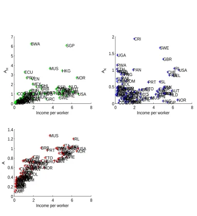
The upper left panel of figure 1 plots the productivity of human capital against income per worker for
ǫ = 0.836. There is a strong positive correlation between the productivity of human capital and income per
worker, which is easily explained by the fact that empirically there is no clear correlation between the income
share of labor and income per worker and a positive relation between output per unit of human capital and
income per worker. On the other hand, there is no obvious relation between the productivity of physical capital
and income per worker (see right panel of figure 1).
If in addition to assuming that factor intensities are identical across sectors we presuppose that productivities are not factor augmenting but Hicks neutral and that the elasticity of substitution is one24, we obtain the
standard model for development accounting that has been used by Klenow and Rodriguez-Clare (1997), Hall
and Jones (1999) and many others.
Ac=
Yc
pσ−σ1Kα cHc1−α
(34)
Ac
AU S =
Yc
YU S
KU S
Kc
α
HU S
Hc
1−α
(35)
In this case one data point per country is sufficient to determineAc, so I follow the tradition to take aggregate
income,Yc, as given. Hall and Jones (and others using this approach) find that cross country differences inAc are large and strongly positively correlated with income per worker. This can be seen clearly from the lower
panel of figure 1, which plots countries’ calibrated productivities against their incomes per worker forα= 0.33,
the average capital income share in my sample.25
Since the Cobb-Douglas case is not directly a limiting case of the general factor deepening model26, I estimate
αusing the HOV-equations to check if a plausible value for this parameter can be obtained.
With a Cobb-Douglas production function the efficient factor use relative to the US is
Df c= VVf U Sf c
KU S
Kc
α
HU S
Hc
1−α
Df U Sand substituting the expression for productivities, the HOV-equations
relative to the US become
Yc
YU S
K
U S
Kc
αH
U S
Hc
1−α
= Yc
YU S
Vf U S
Vf c +F
∗ f c(α)
Vf c
− Yc
YU S
F∗ f U S(α)
Vf U S
+uf c. (36)
Using all 4 orthogonality conditions, ˆα= 0.54, which is implausibly large (the null thatα=0.33 is rejected
at the 1 percent level). However, the J-statistic lets me reject the validity of the orthogonality conditions at the
one percent level. As a consequence, I reestimate the model using only the first two orthogonality conditions.
Now ˆα= 0.69 (again the null that α=0.33 is rejected at the 1 percent level), which is even more implausible
24
The assumption of a unit elasticity of substitution is necessary if productivity is Hicks neutral, if one wants to match the fact
that there is no correlation between factor income shares and income per worker.
25
This calibration is Caselli’s (2005) and is an accounting view point of explaining income differences, because some part of
differences in capital stocks may actually be due to differences in productivity, since in any neoclassical growth model an increase
inAinduces capital accumulation. Hall and Jones (1999) control for this by writing output as a function of the capital output ratio
which is invariant to total factor productivity in the steady state. Results are not very sensitive to the particular approach taken.
26
and once more the orthogonality conditions are unlikely to be satisfied. Next, I estimate α using only the
moment conditions for the human capital content of trade. Now ˆα= 0.23, which is somewhat more realistic but
still the null thatα= 0.33 is rejected, while the orthogonality conditions seem to be valid now. Furthermore,
using only the moment conditions for the physical capital content of trade, ˆα= 1, which does not make much
sense. Summing up, the Cobb-Douglas model with factor deepening performs poorly in terms of fitting the
HOV-equations, especially in the case of physical capital.
Example 2: Conditional Factor Price Equalization (CFPE) & Trefler’s Productivities
If one assumes instead that conditional on measuring endowments in efficiency units, factor prices are
equalized across countries, relative factor productivities can be directly read off from relative factor prices,
ˆ
πc= ˆπU S= ˆπ=
πc
Af c
= πU S
Af U S
. (37)
Sincewc = sHcHcYc and rc = sKcKcYc, I obtain a relationship between factor productivities, factor shares and
factor-income ratios that is similar to Example 1.
Af c
Af U S = sf c
sf U S
Yc
Vf c
YU S
Vf U S
(38)
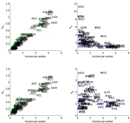
Relative factor productivities are depicted in the upper panels of figure 2. Hence, if conditional factor price
equalization is assumed to hold, rich countries are again more productive in the use of human capital, while
poor countries make more efficient use of physical capital.
The efficient factor use relative to the US is nowDf c=
s
f c
sf U S
Df U Sand the HOV-equations relative to the
US are sf c
sf U S′
Yc
YU S
Vf U S
Vf c =
Yc
YU S
Vf U S
Vf c +
F∗
f c
Vf c−
Yc
YU S
F∗
f U S
Vf U S+uf c, so that they are independent ofθ.
27 Note also that
asǫ→ ∞the HOV equations relative to the US for the factor deepening case (33) converge to CFPE. Hence, the
hypothesis of the aggregate elasticity of substitution being infinite is strongly rejected by the previous estimates.
More evidence against CFPE can be obtained by checking directly the factor use matrices in efficiency units,
which by hypothesis should be equal across countries, i.e. Df U S= AAf U Sf c Df c. In fact, for both factors there is
a significant negative correlation between the average factor use in efficiency units and income per worker, so
that poor countries use more efficient factors per unit of output than rich ones.28
At this point it seems adequate to relate my procedure to Trefler’s (93) paper. His approach is to find a set
of factor productivities that makes the HOV-equations hold exactly under the assumption of CFPE and then to
compare productivity estimates with factor prices. To be more specific, he assumes that there are no Ricardian
technology differences and that conditional factor price equalization holds at the world level (A.10), so that the factor use matrices of all countries are a simple transformation of the one of the US,Df c =A−f c1Df U S and that
all countries have identical input-output matrices, Bc =BU S. Then one can write the factor content of trade
27
This reflects the fact that the values of θ such that CFPE holds at the world level is not unique. The implicit aggregate
elasticity is∞.
28
in efficiency units as
F∗
f c=DU S(I−BU S)−
1(X
c−
X
c′6=c
Mcc′). (39)
Normalizing Af U S = 1 and dropping the equation for the US, the HOV equations in efficiency units (28)
form a system of C−1 independent linear equations in Af c, which can be solved for the unknown factor
productivities.
From (29) we see that ifF∗
f c is small, relative productivities equal relative average products. In fact this is the case in the data if the factor content of trade is computed with the US factor use matrix and as a consequence
productivities computed with Trefler’s method are similar to the ones obtained from (38), which also explains
why Trefler (1993) finds that relative productivities are similar to relative factor prices.29 Rich countries are
measured to have much higher human capital productivities than poor nations, while poor countries tend to have higher productivities of physical capital.30
Example 3: Multiple Cones
If there are multiple cones of diversification, the picture is quite different because the mapping between
en-dowments, factor prices and factor productivities changes its shape, depending on whether a country specializes
or lies in a cone. Again, let us take goods prices as parameters for now.
For countries that specialize in sectori∈ {H, K} the mapping from endowments, factor prices and income
to factor productivities looks similar to Caselli’s.
Af c =
σ
σ−1
1
pi
1
1−αi
sf c
ǫ−ǫ1 Y
c
Vf c
(40)
There are, however, some important differences. First of all, terms of trade effects matter. If goods prices
in the sector in which a country specializes are higher, a lower factor productivity is sufficient to reach a given
income. In addition, if ǫ > 1, factor productivities are decreasing in the weight of capital in production, αi,
which varies across industries, because holding constant factor income shares an increase (decrease) inαiwould
increase income per unit of physical capital (human capital). Since it is held constant, factor productivity
must decrease. If ǫ < 1, factor productivities are increasing in the weight of factors in production because
an increase (decrease) in αi would cause a decrease in output per unit of factor input for given factor income
shares. Holding it constant, factor productivity must increase. Consequently, a highαK implies that - holding
everything else constant - capital abundant countries that specialize in the capital intensive good have high
(low) capital productivities if factors are complements (substitutes).
29
Productivities are not reported, but very similar to figure 2. These results are robust to using the technology matrix of other
countries as reference and to using the true input-output tables of each country in computing the factor content of trade.
30
These results differ from Trefler’s. He finds that rich countries tend to use both labor and physical capital more efficiently than
poor ones. The main reasons seem to be his small sample and his choice of very high depreciation rates of 15% (instead of 6%, as
For countries that lie within the cone of diversification the mapping between endowments, income, prices
and parameters has another form.
AHc=
σ σ−1
αǫ Hp
1−ǫ K −αǫKp
1−ǫ H
αǫ
H(1−αK)ǫ−αǫK(1−αH)ǫ
ǫ−11 sHc
Yc
Hc
(41)
AKc=
σ σ−1
(1−αH)ǫp1K−ǫ−(1−αK)ǫp1H−ǫ
αǫ
K(1−αH)ǫ−αǫH(1−αK)ǫ
ǫ−11 sKc
Yc
Kc
(42)
Factor productivities are again linear functions of factor-output ratios and also of factor income shares.
Terms of trade effects are at work too, but they are more complex than for countries which specialize. Now
productivities are decreasing in the price of the sector that uses the factor intensively. The explanation is again
the Stolper-Samuelson effect. An increase in the price of an industry shifts production towards that sector, and
increases the income share of that factor. If the income share and income per unit of factor are held constant, the factor must have lower productivity.
The lower panels of figure 2 plotAHcandAKc against income per worker for a model with two sectors and
multiple cones, in which goods prices have been solved endogenously for the optimal θ.31 Again, human and
physical capital are estimated to be complements. 39 poor countries specialize in the human capital intensive
sector, while the rest of the world lies in a common cone of diversification. The correlation betweenAHc and
income per worker is again strongly positive and poor countries are still estimated to be more productive in the
use of physical capital.
Using the HOV equations to Compare Model Fit
To see which of the different versions of the model performs best I use an economic measure of performance
- I evaluate the fit of the HOV-equations in efficiency units at ˆθ. I provide the results of the following classical
tests. First the ”sign test” that reports the fraction of observations for which the left hand side (measured
factor content) and the right hand side (predicted factor content) of the HOV-equations (28) have the same sign. Second the ”weighted sign test” that weights observations by the magnitude of factor flows, third the
slope coefficient,β, of a regression of the measured on the predicted factor content, with a theoretical value of
one. Fourth, the R-squared from this regression and finally the ratio of the variances of the measured and the
[image:22.612.169.539.106.181.2]predicted factor content, a measure known as the ”missing trade” statistic.
Table 2 reports the results of these tests. It is quite obvious that the factor deepening model with
comple-mentary factors (ǫ = 0.836) easily outperforms all its competitors - the Cobb-Douglas model (α= 0.33), the
CFPE model and also the - admittedly overly simplistic - two sector multiple cone model in virtually all tests.
For example, the weighted sign statistic is 0.97 for physical capital and 0.96 for human capital for the factor
deepening model, which is by far closer to the theoretical value of one than for any of the other models. It is
also the only model that getsβs of the right sign and roughly correct magnitudes and that does not suffer from ”missing trade”
31α
H = 0.06,αK= 0.77,ǫ= 0.5 andβH= 0.84. Meaningful standard errors for these estimates are hard to obtain, since J is
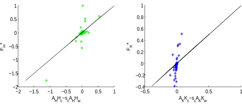
Figure 3 plots the measured factor content against the predicted factor content of trade for the factor
deepening case. The good fit of the model, especially for human capital, is clearly visible, while measured factor
trade is somewhat too large for physical capital. Hence, I conclude that the model by far best supported by the
HOV-equations is the factor deepening model with factor augmenting productivities and weak complementarity
between human and physical capital.
Let me therefore discuss the features of this world in somewhat more detail. Coming back to the upper
panels of figure 1, we see that rich countries are much more productive in the use of human capital than
poor ones. The correlation between AHC and income per worker is 0.432 and strongly significant (P-value: 0.000). There are some outliers, like Botswana and Singapore, which have extremely low labor income shares
in the data and therefore very high human capital productivities. Since the data quality on labor income
shares is not very good, this should be taken with some caution. The ratio of human capital productivity of
the 90th to the 10th percentile is 10.72. In the case of physical capital, there is a no clear relation between
factor productivity and income per worker. The correlation between AKc and income per worker is slightly
negative (-0.031) but insignificant (P-value: 0.767). The ratio of physical capital productivity of the 90th to
the 10th percentile is 10.72. A number of very poor African economies are measured to have very high capital
productivities, which is due to their extremely low capital output ratio. When we disregard these countries,
there is a positive relation between capital productivity and income per worker, with Sweden, the UK, Ireland,
Switzerland, France, Belgium and the US measured to have very high capital productivities. While it is quite intuitive that rich countries are much more efficient in their use of human capital, it is less clear, why a number
of very poor African countries should be so productive in the use of physical capital. The fact that some of
the poorest countries in the world use so little physical capital in production could well reflect distortions in
capital markets, like high tariffs on capital goods and malfunctioning of credit markets instead of high capital
productivities. In this world there are incentives for human capital to move to rich countries and for capital to
move to poor ones because returns in physical units are not equalized.
A further feature of the factor deepening world is that the physical to human capital ratios in efficiency
units are quite similar across countries. This is due to the fact that rich countries, which have large physical to
human capital ratios, have very high human capital productivities and that there is no clear relation between
capital productivity and income per worker.
Turning to the estimate of the elasticity of substitution, note that my estimates are similar to those of Antr`as
(2004), who estimates the elasticity of substitution between labor and capital for the US aggregate production
function from time series data allowing for biased technological change. He finds values in the range of 0.5 to
0.9, so my estimates are consistent with time series evidence for the US.
Another point worth mentioning is the relation of my findings to the extensive literature on the
HOV-equations. Even though it is well known that these relations apply to a wide class of models, it seems interesting
that the model that actually best fits the HOV-equations (at least in the relatively restrictive class of models