Vector autoregression with varied frequency data

Munich Personal RePEc Archive

Vector autoregression with varied

frequency data

Qian, Hang

Iowa State University

October 2010

Online at

https://mpra.ub.uni-muenchen.de/34682/

Vector Autoregression with Varied Frequency Data

Hang Qian1

Abstract

The Vector Autoregression (VAR) model has been extensively applied in

macroeconomics. A typical VAR requires its component variables being

sam-pled at a uniformed frequency, regardless of the fact that some macro data

are available monthly and some are only quarterly. Practitioners invariably

align variables to the same frequency either by aggregation or imputation,

regardless of information loss or noises gain. We study a VAR model with

varied frequency data in a Bayesian context. Lower frequency (aggregated)

data are essentially a linear combination of higher frequency (disaggregated)

data. The observed aggregated data impose linear constraints on the

au-tocorrelation structure of the latent disaggregated data. The perception of

a constrained multivariate normal distribution is crucial to our Gibbs

sam-pler. Furthermore, the Markov property of the VAR series enables a block

Gibbs sampler, which performs faster for evenly aggregated data. Lastly,

our approach is applied to two classic structural VAR analyses, one with

long-run and the other with short-run identification constraints. These

ap-plications demonstrate that it is both feasible and sensible to use data of

different frequencies in a new VAR model, the one that keeps the branding

1

of the economic ideas underlying the structural VAR model but only makes

minimum modification from a technical perspective.

Keywords: Vector Autoregression, Bayesian, Temporal aggregation

1. Introduction

The Vector Autoregression (VAR) proposed by Christopher Sims (1980)

is a workhorse model for forecasting as well as studying cause and effect in the

macroeconomy. An autoregression model implicitly assumes data are

sam-pled at the same frequency since variables at datetare regressed on variables

dated at t−1, t−2, etc. However, macroeconomic data are not always

ob-served at a uniformed frequency. First, each series can be sampled at its own

frequency. For example, the best available data of GDP is quarterly, while

that of the CPI is monthly, that of financial asset returns might be daily or

more frequent. Second, for a given variable, recent data may be observed

at a higher frequency while historical data may be coarsely sampled. For

instance, quarterly GDP data are not available until 1947. In the presence

of varied frequency data, a VAR practitioner aligns the variables either by

aggregating the data to a lower frequency or imputing the high frequency

data with heuristic rules. The former method discards valuable information

in the fine data while the latter introduces noises to the data.

By far the most popular model that handles mixed frequencies data is

the Mi(xed) Da(ta) S(ampling), or MIDAS, regression introduced by Ghysels

et al. (2007), Andreou et al. (2010). The MIDAS regression projects high

fre-quency data onto low frequencies data with a tightly parameterized weighing

volatil-ity prediction (e.g., Ghysels et al., 2006), it quickly gains popularvolatil-ity among

macroeconomists for improving real-time forecast of key economic variables.

See Clements and Galvao (2008, 2009), Marcellino and Schumacher (2010),

and Kuzin et al. (2011) for applications.

In the MIDAS regression, the parsimonious declining weights, such as

Almon lag polynomial or normalized Beta density, impose a priori structure

on the decaying pattern of the regression coefficients. It is true that such a

structure is necessary when the aggregation periods are long, say using daily

variables to predict quarterly outcomes. Otherwise there will be parameter

proliferation. However, for many macroeconomic data aggregation periods

are relatively short, say monthly-quarterly, or quarterly-annual aggregation.

It is both feasible and sensible to adopt a fully data-driven dynamic model like

VAR. We name our model as the Var(ied) Da(ta) S(ampling), or VARDAS,

regression, implying we follow the tradition of using the established VAR

model in macroeconomic studies.

The MIDAS regression is raised mainly in the context of economic

fore-casting. The VARDAS model, however, can be used for both forecasting and

characterizing dynamic nexus among macroeconomic variables. In fact, the

VARDAS model is analogue to a reduced-form VAR. Once its parameters

are routinely estimated, it can be restored to a structural model for the

im-pulse response analysis. The economic insights used for identifying structural

shocks remain unchanged. In fact, it effectively weakens many short-run

identification assumptions such as zero contemporaneous effects, since our

VARDAS model operates on an autoregression with higher frequency data

The VARDAS model is built upon the VAR model, but also takes the

temporal aggregation into consideration. The effects of temporal aggregation

have been extensively studied in literature over decades. Amemiya and Wu

(1972), Tiao (1972), Tiao and Wei (1976), Marcellino (1999), Breitung and

Swanson (2002) discuss, as a result of temporal aggregation, the change of

lag orders of ARMA models, information loss in estimation and prediction,

dynamic causality and integration relations among aggregated variates, etc.

Silvestrini and Veredas (2008) provide a comprehensive review on the theory

of temporal aggregation of time series models. The focus of our paper is

not on the relationship between the aggregated model (estimated by low

frequency data) and the disaggregated model (estimated by high frequency

data, if available), but instead on an empirical concern: how to estimate a

disaggregated model if some data are aggregated?

This question itself is not new. Under the frequentist framework, the

mixed frequency VAR and a related factor model have been explored by

Zadrozny (1988), Mittnik and Zadrozny (2004), Mariano and Murasawa

(2003, 2010), Hyung and Granger (2008). The wisdom is to recast the VAR

model with temporally aggregated variates into a state space model so that

the likelihood function can be recursively evaluated by the Kalman filter.

However, the main difficulty is that a VAR model typically contains many

coefficients and numerical algorithms such as the quasi-Newton have limited

ability to implement the maximum likelihood estimation.2

2

As is noted by Chen and Zadrozny (1998), Kalman filter method may perform poorly

or not at all on a larger model. In applications, variables included need to be carefully

The mixed frequency VAR with the Kalman filter is essentially the

fre-quentist version of the VARDAS model. The VARDAS model is raised in a

Bayesian framework mainly because the Gibbs sampler with data

augmenta-tion is ideal for latent variable models. The large number of parameters does

not pose major computational difficulties in that conditional on the latent

disaggregated data it is a standard VAR model, with its parameters sampled

in a way analogue to the linear regression model. The crux of our Gibbs

sampler is a constrained multivariate normal distribution characterizing the

posterior conditionals of the latent disaggregated variables. Furthermore, a

blocking strategy that takes advantage of the Markov property of the VAR

series accelerates the sampler, making the algorithm feasible even for a larger

scale model.

Compared with the mixed frequency VAR with the Kalman filter, the

VARDAS model is flexible and friendly to practitioners. It allows each

com-ponent series in the VAR system being sampled at its own frequency and

may change its frequency at any time. Though it is possible to redesign the

state space representation of the frequentist model to reach this level of

gen-erality, the design must be tailored and finished by the practitioners, with

no guarantee of numerical feasibility of maximizing the likelihood. However,

values need to be carefully set. Many authors find it crucial to demean the data before

applying the Kalman filter. Mittnik and Zadrozny (2004, p.7) report that “the MLE

was not automatic and needed intervention”. Aruoba and Scotti (2009) discuss in detail

the two steps they use to select the initial values before applying the BFGS numerical

maximzation. Mariano and Murasawa (2010) use the EM algorithm to obtain an initial

the VARDAS model only requires users to provide the data and specify the

aggregation structure, while the estimation is as routine as a standard VAR

model.

Our research is closest to a Bayesian estimation of the VAR model with

mixed or irregular spaced data proposed by Chiu, Eraker, Foerster, Kim,

and Seoane (2011, hereafter CEFKS). However, our econometric model and

sampling techniques have two genuine differences from those in CEFKS.

First, CEFKS assume the lower-frequency data are the result of sampling

everykperiods from the high frequency variable. For example, quarterly data

are treated as variables sampled at the end of March, June, September and

December. However, most macroeconomic data do not seem to be generated

in that fashion. Flow variables such as quarterly GDP is the sum of the

latent “monthly GDP”in a quarter. Stock variables such as the monthly

CPI are more reasonably viewed as an average of the latent “weekly CPI”

in a month instead of the price level in the last week of a month.3 _{Even if}

some variables are really sampled only once in a month, there is no reason to

expect it realizes in the last week. If the realized date is the first week,

auto-correlations and cross-auto-correlations imply a different posterior distribution of

3

in the literature, stock variables are defined as those sampled every k periods from the latent high frequency variables. The examples provided for stock variables are “rates

and indexes” such as interest rate, unemployment rate and CPI (Silvestrini and Veredas,

2008). However, all of them seem to be generated by averaging the latent variables in the

k periods. Some financial data such as the S&P 500 index and exchange rates in a week or month do have their last-trading-day data available, but the averaged data are offered

the latent variable.

CEFKS address the missing disaggregated data in the VAR system. Data

aggregation problems bear some similarities to the traditional missing data

problems, but a genuine difference is that data aggregation imposes

lin-ear temporal constraints on the disaggregated variates, which exhibit

auto-correlations and cross-auto-correlations as well. So the posterior latent variables

follow a constrained, conditional multivariate normal distribution.

Second, in the CEFKS sampler, single-period (say, date t) latent

disag-gregated data are drawn conditional on all other latent values. In the VAR(1)

model, two neighbors (that is, values in date t−1 and t+ 1) are relevant.

Though this is a valid sampler, the excessive length of the MCMC chain

might result in its slow mixing. Our method is to sample latent variables of

all periods at one time, which reduces the nodes and improve the mixing.

We also propose a block Gibbs sampler, which does increase the nodes on

the MCMC chain, but the block size is at the discretion of the user so as to

reach a balance between the sampling efficiency and speed.

The rest of the paper is organized as follows. Section 2 specifies of the

VARDAS model. Section 3 explains the Gibbs sampler and Section 4

pro-poses an alternative block sampler. Section 5 extends the baseline

econo-metric model to various aggregation types other than simple summation and

averaging. Section 6 illustrates our approach by two classic applications of

structural VAR model, one with long-run and the other with short-run

2. The model

Assume the k dimensional latent {Y_t∗}T_t=1 follow a covariance-stationary

reduced-form VAR(p) process:

Y∗_t =c+

p

X

i=1

Φ_iY_t−i∗ +εt,

where εt∼N(0,Ω). The reference time unit is t, which indexes the highest

frequency data in the VAR system. The (column) vector Y∗_t is unobservable since some of the component series may be observed at some lower frequencies

and are allowed to change sampling frequencies at any time. The

book-keeping convention of observed data is specified as follows. Let {Y∗ t }

T t=1 be

a component series (say, the first variable) in the VAR system. Suppose in

some time interval [a, b], 1≤a≤b≤T,a, b∈N_{, disaggregated latent values}

Y_a∗, Y_a∗₊₁...Y_b−∗₁, Y_b∗ are aggregated into a single observable variate Ya,b ≡

Pb−a

j=0Ya∗+j. We then construct a data series{Yt}Tt=1 such that Ya=Ya+1...=

Yb−1 =N.A.andYb =Ya,b. As a special case,a =bimplies the disaggregated

value (highest frequency data) is observed. The data series {Yt}Tt=1 contains

all the available information with respect to the latent {Y∗ t }

T

t=1. Though

data of various frequencies may be present in {Yt}Tt=1, there is no ambiguity

since counting a run of N.A. preceding a data point reveals the aggregation

structure. Sometimes high frequency data are grouped into low frequency

data by averaging instead of summation, sayYa,b≡ _b−a1₊₁Pb−a_j=0Ya∗+j. In that

case, we simply record Yb = (b−a+ 1)Ya,b so that it becomes equivalent

to aggregation by summation. More complicated data averaging types, such

as weighed, noisy, missing and nonlinear aggregation, will be discussed in

Repeat the above process for each of the k component variables in the

VAR system, we obtainkdata series. Ak-by-T data matrixYis constructed by pooling all the data series. Each row is a component data series and

each column is the data of k variables at a given time. Clearly Y contains many N.A. entries, and we define a k-by-T logical matrix E such that the

(i, j) entry of E equals zero if the corresponding entry of Y is N.A., and equals one otherwise. The notation −→E vectorizes the matrix E column by

column, which will be used to select entries of a matrix (vector) to form a

submatrix (subvector). Similarly, the operator −→Y vectorizes the matrix Y.

Let Y∗ = (Y∗

1, ...,YT∗), and

−→

Y∗ vectorizes the matrixY∗.

Essentially our task to estimate model parametersΘ≡ {c,Φ₁, ...,Φp,Ω}

and recover the latentY∗ with the observation matrixY. A Bayesian frame-work is adopted since the Gibbs sampler with data augmentation can

conve-niently handle models with latent variables. The Gibbs sampler only requires

the full posterior conditionals of model parameters as well as latent

disag-gregated variables. Clearly, conditional on the latent Y∗, this is a standard VAR model. By convention, treat the initial Y₁∗, ...,Y_p∗ as given, so the VAR

model is equivalent to a seemingly unrelated regression model.4

4

Strictly speaking, the VAR model is reduced to a multiple-equation linear regression

model only if we neglect the contribution of the initial p observations to the likelihood. Otherwise the posterior conditionals of c_,Φ_{1, ...,}Φ_{p do not have a closed form.}

How-ever, conditioning on initial values is also commonly applied in the frequentist framework. Hamilton (1994, p. 291) notes that “Vector autoregressions are invariably estimated on the

basis of the conditional likelihood function ... rather than the full-sample unconditional

likelihood”, so that maximizing the conditional likelihood is equivalent to OLS regressions

Denote a 1-by-(kp+ 1) vector xt =

1 Y_t−∗′₁ ... Y∗′_t−p

, and a k

-by-(kp+ 1)k block-diagonal matrix X_t =      xt . .. xt     .

Letβ = (c,Φ₁, ...,Φp)′. With a conjugate proper prior

− →

β ∼_N(µβ,Vβ),

Ω−1 ∼_{W ishart(Ω, ν), where the operator} −→_{β vectorize β, we have}

− →

β |· ∼_{N(Dβdβ,Dβ) ,}

Ω−1|· ∼_{W ishart Ω, ν,}

where

D_β =

T

X

t=p+1

X′_tΩ−1X_t+V−_β1 !−1

,

d_β =

T

X

t=p+1

X′_tΩ−1Y_t∗+V−_β1µβ,

Ω= "

Ω−1+

T

X

t=p+1

Y_t∗−X_t−→β Y_t∗−X_t−→β′

#−1 ,

ν =T −p+ν.

3. Posterior disaggregated variables

In this section, we describe how to sample the latent−Y→∗ from its posterior

conditional distribution. Before presenting our sampler formally, we motivate

our approach by a highly simplified scenario in which the system contains

only one variable following an monthly AR(1):

Y_t∗ =φY_t−∗₁+εt, εt ∼N 0, σ2

Suppose we only have one quarterly observation Y1,3 = Y1∗ +Y2∗ +Y3∗

and one monthly observation Y4 = Y4∗. Conditional on φ, σ2, Y1,3, Y4 we

are interested in the posterior distribution of Y−→∗ ≡ (Y₁∗, Y₂∗, Y₃∗, Y₄∗)′. For

notational conciseness, we leave conditioning onφ, σ2 _{implicit. By our}

book-keeping convention, −→Y = N.A., N.A., Y1,3, Y4 ′

, −→E = (0,0,1,1)′.

First note that ifY∗

1 comes from the stationary distribution of the AR(1)

process, then −Y→∗ ∼ _{N(0,Γ), where the (i, j) entry of Γ equals} σ2

1−φφ |i−j|_.

However, −Y→∗ is binded by two linear constraints. First, Y∗

1 +Y2∗+Y3∗ must sum up to the known Y1,3. Second, Y4∗ must equal to the known Y4. That

implies−Y→∗ follows a constrained multivariate normal distribution, which can be represented as the product of a conditional normal and a degenerated

distribution. To this end, construct a transformation matrix such that

A=        

1 0 0 0

0 1 0 0

1 1 1 0

0 0 0 1         .

ThenA−Y→∗ = Y₁∗, Y₂∗, Y1,3, Y4 ′

∼_N(0,AΓA′_).

It follows that

(Y₁∗, Y₂∗)′Y1,3, Y4 ∼N h

Γ01Γ−₁₁1· Y1,3, Y4 ′

,Γ00−Γ01Γ−111Γ10 i

,

where Γ01 is the submatrix of AΓA′ with rows selected by 1 −

− →

E, and columns selected by−→E, andΓ00,Γ11,Γ10are defined similarly. Practically, in a matrix-based computational environment such as MATLAB, R or GAUSS,

Lastly, (Y₃∗, Y₄∗)′Y₁∗, Y₂∗, Y1,3, Y4 are degenerated sinceY3∗ =Y1,3−Y1∗−

Y∗

2 andY4∗ =Y4. The posterior distribution of

−→

Y∗is completely characterized by the product of (Y₁∗, Y₂∗)′Y1,3, Y4 and (Y3∗, Y4∗)

′

Y₁∗, Y₂∗, Y1,3, Y4, so the

problem is resolved.

This example demonstrates our idea of sampling the latent −Y→∗. The

disturbances εt are multivariate normal, so

−→

Y∗ also follows kT dimensional multivariate normal. If we use a kT-by-kT matrix A to linearly transform

−→

Y∗, the resulting matrix A−Y→∗ is multivariate normal as well. The purpose of this transformation is to relate the disaggregated and aggregated data.

The latter is known so that the former follows a conditional normal

distribu-tion. Recall that the logical vector −→E indicated which entries in −→Y contain

aggregation information and which do not. So −→E will be used to construct our conditional normal distribution. Our procedure is formally presented as

follows.

If the initialY∗′₁, ...,Y_p∗′come from the stationary distribution of the VAR

system, then−Y→∗ ∼_{N(µ,Γ), whereµ= (µ}′

1, ..., µ′1)

′

,µ1 = (Ik−Ppi=1Φi)−1c.

The kT-by-kT covariance matrix Γ is given by

Γ=        

Γ0 Γ′1 ... Γ′T−1

Γ1 Γ0 ... Γ′T−2

...

ΓT−1 ΓT−2 ... Γ0         ,

where the autocovariance matrixΓ_j =E(Y_T −µ) (Y_T−j −µ)′,j = 0,1,2, ...

can be recursively computed by

Γ_j =

p

X

i=1

As for the initial Γ0, ...,Γp−1, we compute a kp-by-kp matrix G such that

− →

G = [Ik2_p2 −(F⊗F)]−1

− →

∆, where F =   Φ

C 

, Φ= (Φ1, ...,Φp), C =

Ik(p−1) 0k(p−1),k

, and ∆is akp-by-kpmatrix of zeros except for its first (northwest)k-by-k submatrix beingΩ. The firstk rows ofGis (Γ0, ...,Γp−1).

ThekT-by-kT transformation matrixAcan be constructed by examining the logical matrix E. First, let the main diagonal of A be ones and other

elements be zeros. Second, examine each row of the logical matrix E. Sup-pose we are reading row i and column j of E (i = 1, ..., k;j = 1, ..., T). If

the (i, j) entry is zero, skip and proceed to column j + 1 (or conclude this

row). Otherwise, (i, j) entry being one implies a temporally aggregated data

is observed. So we search column j−1, j−2, ... for a run of zeros. Suppose

there are M zeros (M ≥ 0) in a row immediately before column j; we then

add M ones to A. For M >0, the locations inA are row (j−1)k+i, col-umn (j −1)k+i−mk, m = 1, ..., M. Note that M = 0 implies one-period

trivial aggregation.

The new series A−Y→∗ transforms the original series −Y→∗ in such a way

that for a (M + 1)-period temporal aggregation, the first M disaggregated

variates are retained, while the last disaggregated variate is replaced by the

sum of the disaggregated variates in the M + 1 periods. As a special case,

for a one-period aggregation, the variate is simply retained. Clearly, A−Y→∗

can be classified into two blocks: the latent disaggregated variates block

and the observed variates block. The latter have their realizations contained

A−Y→∗ ∼_N(Aµ,AΓA′_{), and}

−→

Y₀∗

−→Y,Θ ∼_N

h

η0+Γ01Γ−111 _−→

Y₁−η1

,Γ₀₀−Γ01Γ−111Γ10 i

,

where Y−→∗₀ is the subvector of AY−→∗ selected by the logical vector 1 −−→E,

namely the latent disaggregated variates block. The vector −Y→₁ has double identities: as a random vector, it is the subvector of A−Y→∗ selected by −→E,

namely the observed variates block; as a realization of that random vector,

it is exactly the subvector of −→Y selected by −→E (simply the non- N.A. part

of our data −→Y). η0 and η1 are two subvectors of Aµselected by 1−

− →

E and

− →

E respectively. Γ01 is the submatrix of AΓA′ with rows selected by 1−

− →

E, and columns selected by −→E, andΓ₁₁,Γ₀₀,Γ₁₀ are defined similarly.

Lastly, Note that in the transformation we squeezed out one

disaggre-gated variate at the end of the aggregation periods, and replaced it with an

aggregated data. Treat one period aggregation as squeezing out and filling in

the same variate. Those squeezed-out variates, denoted as −−→Y∗

−1, correspond

to the subvector of−Y→∗ selected by−→E. However,−−→Y∗₋₁

−Y→₀∗,−→Y, θ is degenerate, since it must equal to the difference between the aggregated value and the

sum of the rest disaggregated values. Note that −Y→∗₀ has another identity,

namely the subvector of −Y→∗ _{selected by 1−}−→_{E, which implies the two}

vec-tors −Y→₀∗ and −−→Y∗₋₁ cover all the elements in the latent −Y→∗. In other words,

by sampling in turn −Y→∗

0

−→Y, θ from a conditional normal distribution and

−−→

Y∗₋₁

−Y→∗₀,−→Y, θ from a degenerated distribution, we obtain the posterior con-ditional sample of −Y→∗_{. That finishes the cycle of the Gibbs sampler to the}

4. Gibbs sampler with Blocks

The sampling procedure in the previous section allows us to draw the

latent disaggregated values all at once. For macroeconomic data with

sev-eral hundred observations, the sampler is workable on an ordinary desktop

computer. However, if we need to handle a large dataset which contains ten

thousand observations, the above procedure requires handling large matrixes

and their inversion, which slow down the sampling speed and create burden

on the computer memory. In this section we propose an alternative sampler

which divide latent variables into blocks. It is fast and memory-efficient, at

the price of increasing nodes on the MCMC chain.

The idea of this approach is to explore the Markov property of the series

to simplify conditional distributions and thus reduce the size of matrixes.

To fix ideas, consider again the simple scenario in Section 3. The system

contains only one variable following a monthly AR(1):

Y_t∗ =φY_t−∗₁+εt, εt ∼N 0, σ2

.

Suppose we observe two quarterly observations Y1,3 = Y1∗ +Y2∗ +Y3∗,

Y4,6 = Y4∗ +Y5∗ +Y6∗ and one monthly observation Y7 = Y7∗. Conditional

onφ, σ2, Y1,3, Y4,6, Y7 we are interested in the posterior distribution of

−→

Y∗ ≡

(Y∗

1, ..., Y7∗)

′

. If we sample the latent variates all at once, we need to work on

a 7-by-7 transformation matrix and covariance matrix.

Now we partition the seven latent variables into three blocks and

need to specify the posterior conditional of

(Y₁∗, Y₂∗, Y₃∗)′Y1,3, Y4,6, Y7, Y4∗, Y5∗, Y6∗, Y7∗ ,

(Y₄∗, Y₅∗, Y₆∗)′Y1,3, Y4,6, Y7, Y1∗, Y2∗, Y3∗, Y7∗ ,

Y₇∗Y1,3, Y4,6, Y7, Y1∗, ..., Y6∗ .

The last block has a degenerate distribution, so we focus on the first

two blocks. To sample (Y∗

1, Y2∗, Y3∗)

′

conditional on all other disaggregated

values, we note that the Markov property of an AR(1) process implies that

once we know Y∗

4, further knowledge on Y5∗, Y6∗, Y7∗ is irrelevant. So it is equivalent to work on (Y₁∗, Y₂∗, Y₃∗)′Y1,3, Y4∗. By a linear transformation,

Y∗

1, Y2∗, Y1,3, Y4∗ ′

follows a multivariate normal, so we first sample (Y∗

1, Y2∗)

′

conditional on Y1,3, Y4∗, and then sample the degenerated Y3∗, a procedure

essentially the same as that in the previous section. Note that this process

only requires us to construct a 4-by-4 transformation matrix and covariance

matrix.

Similarly, to sample (Y₄∗, Y₅∗, Y₆∗)′ conditional on all other disaggregated

values, we work on (Y∗

4, Y5∗, Y6∗)

′

Y4,6, Y3∗, Y7, with a 5-by-5 transformation

matrix A which takes (Y₃∗, Y₄∗, Y₅∗, Y₆∗, Y₇∗)′ into Y₃∗, Y₄∗, Y₅∗, Y4,6, Y7 ′

with

the distributionN0,₁σ_−φ2 AΓA′, where the (i, j) entry ofΓequalsφ|i−j|_{. So}

we first sample (Y₄∗, Y₅∗)′Y4,6, Y3∗, Y7 from a conditional normal distribution

and then sample the degenerated Y∗

6.

This example illustrates the ideas of our block Gibbs sampler, though the

computational saving is mild in that we only have two quarterly observations.

However, if we instead have 100 quarterly observations, the computational

need to construct an at least 300-by-300 transformation matrix. However,

we can group 3 latent monthly variables in a block, say Y∗

t , Yt∗+1, Yt∗+2 ′

,

t = 1,4,7, ...,298, with the quarterly observation Yt,t+2. The Markov

prop-erty implies that Y∗

t , Yt∗+1, Yt∗+2 ′

conditional on all the other disaggregated

variates is equivalent to that conditional on Y_t−∗₁, Y_t∗₊₃ (with proper

modi-fications to the two ends of the series). Once we build a 5-by-5 matrix A that transforms Y_t−∗₁, Y_t∗, Y_t∗₊₁, Y_t∗₊₂, Y_t∗₊₃′ into Y_t−∗₁, Y_t∗, Y_t∗₊₁, Yt,t+2, Yt∗+3

′

,

we can sample Y∗ t , Yt∗+1

′

from a conditional normal andY∗

t+2 from a

degen-erated distribution. Furthermore, the stationarity of the series implies the

co-variance matrix of Y∗

t−1, Yt∗, Yt∗+1, Yt,t+2, Yt∗+3 ′

is time invariant, which offers

another major computational advantage in addition to the reduced matrix

dimensions.

Also note that the size of the block is not necessarily equal to an

ag-gregation cycle. For example, it is legitimate to partition the series as

Y_t∗, ..., Y_t∗₊₅′, t = 1,7,13...,295. Larger block size increases computation

time, but reduces the nodes on the MCMC chain as well and thus improves

the mixing of the chain. If the entire series are treated as one block, we go

back to the sampler specified in Section 3.

In a general VAR(p)-based VARDAS model, the blocking strategy still

applies. Let Y,E,A, µ,Γ as defined in Section 3. Suppose we intend to sample Y∗_t,Y_t∗₊₂...,Y∗_t+j in one block, conditional on disaggregated draws

of all other blocks. The integerj should be picked such that all the

aggrega-tion constraints in the time interval [t, t+j] does not involve disaggregated

variates outside that time interval. For example, if monthly, quarterly,

the actual size might be 12,18,24, and so on. The Markov property of the

VAR(p) model suggest that we only need to use the joint distribution of

Y∗_t−p, ...,Y∗_t...,Y_t∗_+j, ...,Y∗_t+j+p to formulate the conditional normal distri-bution. Let ee be ak-by-(j+ 1) submatrix of E using its columns t to t+j. Lete= (ι,ee, ι), whereιis ak-by-pmatrix of ones. Then we can use the

vec-torized−→e to select submatrixes to form the conditional normal distribution.

−→

Y∗₀

−→Y, θ ∼_N

h

η0 +Γ01Γ−111 _−→

Y₁−η1

,Γ₀₀−Γ₀₁Γ−₁₁1Γ₁₀i,

where Y−→∗₀ is the subvector of AY−→∗ selected by the logical vector 1 − −→e,

namely all the unobserved disaggregated variates within Y∗_t,Y∗_t+2...,Y∗_t+j. The vector −Y→1 is the subvector of

− →

Y selected by −→e. η0 and η1 are two subvectors ofAµselected by 1− −→e and−→e respectively. Γ01is the submatrix of AΓA′ with rows selected by 1 − −→e, and columns selected by −→e, and

Γ11,Γ00,Γ10 are defined similarly.

Of course, practitioners does not necessarily need to start from those giant

matrixY,E,A, µ,Γand use−→e to select submatrixes. The joint distribution of Y_t−p∗ , ...,Y_t∗...,Y∗_t+j, ...,Y_t∗_+j+pcan be worked out directly by examining

the VAR(p) covariance structure. Furthermore, in a balanced aggregation

the transformation matrix and covariance matrix are time invariant, so that

it only needs to be computed once per Gibbs sampler cycle.

5. Other aggregation types

Macroeconomic data may exhibit more complicated aggregation types

other than summation and simple average. In this section, we extend the

VARDAS model to various aggregation types that an empirical researcher

5.1. Weighed aggregation

In the baseline model, the time interval [t, t+ 1] is equidistant over time.

However, calender days vary in a month, and working days are affected by

holidays. Suppose latent daily values of some variable are simple-averaged to

generate latent quarterly data and observable annual data. Assume 66,66,66,60

working days in the four quarters, and then the latent quarterly values

{Y∗ t }

T

t=1 are linked to the annual data

Y4i+1,4i+4

T /4−1

i=0 by the relation

Y4i+1,4i+4 = ₂₅₂66Y4∗i+1+25266Y

∗

4i+2+25266Y

∗

4i+3+25260Y

∗

4i+4.

In a general setting, let {Y∗ t }

T

t=1 be a component series in the VAR

system. Suppose in some time interval [a, b], disaggregated latent values

Y∗

a, Ya∗+1...Yb−∗1, Yb∗ are grouped into an aggregated observed data Ya,b ≡

Pb−a

j=0ωa+jYa∗+j, where {ωt}T_t=1 is a deterministic weight series. In the above

example, the weight series looks like ...,₂₅₂66,₂₅₂66,₂₅₂66,₂₅₂60, ... . The data

se-ries {Yt}T_t=1 and the matrixesY,Y∗,Eare constructed in the same way as in

Section 3, but the transformation matrixA needs to incorporate the weights information. The matrix A can be constructed based on a kT-by-kT

iden-tity matrix. Then we examine the logical matrix E row by row to modify

A as appropriate. Suppose we are reading row i and column j of E. If the (i, j) entry is zero, skip and proceed to column j+ 1 (or conclude this row).

Otherwise, we search columnj−1, j−2, ...for a run of zeros. Suppose there

are M zeros in a row (M ≥0) immediately before column j. By reading the

weight series{ωt}T_t=1 of variablei, we extractωj, ωj−1, ..., ωj−M and add them

to A. The locations in A are row (j −1)k+i, column (j−1)k+i−mk,

5.2. Differenced data and weighed aggregation

The VAR model in use is covariance stationary. However, many

macroe-conomic variables contain unit roots. It is common to put the first-differenced

variables in the VAR system, though in the current model cointegration

rela-tions and error correction terms are not included. The VARDAS model with

cointegration is left for future research.

Consider an example. Let {Y∗ t }

T

t=1 be the latent monthly GDP series

and we actually put ∆Y∗

t ≡ Yt∗−Yt−∗1 as a component variable in the VAR model. We observe the quarterly GDP series Yt,t+2 =Yt∗+Yt∗+1+Yt∗+2, t=

1,4,7, .... Define the quarterly-differenced data ∆3_Y

t,t+2 =Yt,t+2−Yt−3,t−1.

The observable quarterly-differenced data and the unobservable

monthly-differenced data are linked by the relation

∆3Yt,t+2 = 3 X

j=1

Y_t∗−Y_t−∗₃

= 3 X

j=1

∆Y_t∗+ ∆Y_t−∗₁+ ∆Y_t−∗₂

= ∆Y_t∗₊₂+ 2∆Y_t∗₊₁+ 3∆Y_t∗+ 2∆Y_t−∗₁+ ∆Y_t−∗₂.

In other words, the observed quarterly GDP growth series is a weighed sum

of the unobserved monthly GDP growth series. Similarly, suppose the

ag-gregated value is formed by taking average instead of summation, that is,

Yt,t+2 = 1₃ Yt∗+Yt∗+1+Yt∗+2

. The quarterly-monthly differenced data are

linked by the relation

∆3Yt,t+2 = 1 3∆Y

∗ t+2+

2 3∆Y

∗

t+1+ ∆Yt∗+

2 3∆Y

∗ t−1+

1 3∆Y

∗ t−2.

In principle, the approach handling weighed averaged data in the previous

data in the data series {Yt}T_t=1 every three entries (with other entries being

N.A.). As for the transformation matrix A, suppose we are reading row

i and column j of E and (i, j) is a non-zero entry. Then for summation-type aggregation we add (1,2,3,2,1) to A at row (j −1)k+i and column (j−1)k+i−mk, m = 0, ...,4. The rest sampling procedure remains the

same.

In practice, it is preferable to estimate the differenced-data VARDAS

model using a block Gibbs sampler.5 _{However, in this case the block sampler}

differs slightly from the previous one. If we define an aggregation cycle as the

periods that level data aggregate (say 3 months in the above example), the

aggregation of differenced data spans across two aggregation cycles, which

implies that two aggregated data are relevant when we sample a block of

variables in an aggregation circle.

5

It seems that there are some numerical issues if the disaggregated, differenced data

are sampled all at once. Consider a univariate AR(1) with φ = 0.5, σ2

= 1. Let the

covariance matrix of T observations be Γ_{, where the (}i, j) entry of Γ _{equals 1}σ2

−φφ

|i−j|_.

Construct the transformation matrixA_{with weights (1},2,3,2,1) assigned as appropriate. The transformed covariance matrixAΓA′ _{is positive definite in theory. However, it seems}

that when T is larger than 100, MATLAB cannot perform the cholesky decomposition and produces a non-positive definite error, though we know theoretically the cholesky

factor in this case is AL_{, where} LL′ ₌Γ_{. The puzzle is that regardless of} T MATLAB can always cholesky decompose Γ _and AΓA′ _{for level-data aggregation specified in the}

previous section. We are not aware of the source of this numerical problem, so currently we

estimate the differenced-data model using the blocking strategy, in which the transformed

For illustration, consider again a monthly AR(1) model such that

∆Y_t∗ =φ·∆Y_t−∗₁+εt,

while only quarterly-differenced variables ∆3_Y

t,t+2, t = 4,7,10, ... are

ob-served. Suppose we intend to sample the block ∆Y∗

t ,∆Yt∗+1,∆Yt∗+2

condi-tional on all the other monthly-differenced data as well as quarterly-differenced

data. In this case, two aggregated values ∆3_Y

t,t+2, ∆3Yt+3,t+5 binds disag-gregated ∆Y_t∗,∆Y_t∗₊₁,∆Y_t∗₊₂ such that

∆Y_t∗₊₂+ 2∆Y_t∗₊₁+ 3∆Y_t∗ = ∆3Yt,t+2−2∆Yt−∗1−∆Yt−∗2,

2∆Y_t∗₊₂+ ∆Y_t∗₊₁ = ∆3_Y

t+3,t+5−∆Yt∗+5−2∆Yt∗+4−3∆Yt∗+3.

In others words, ∆Y_t∗,∆Y_t+1∗ ,∆Y_t∗₊₂ follows a condition normal

distribu-tion subject to two linear constraints. So we first explore the Markov

prop-erty of AR(1) process and use the (unconditional) joint normal

distribu-tion of ∆Y_t−∗₁,∆Y_t∗,∆Y_t∗₊₁,∆Y_t∗₊₂,∆Y_t∗₊₃ to find out the distribution of

∆Y_t∗,∆Y_t∗₊₁,∆Y_t∗₊₂ conditional on all the other disaggregated data. Then

we build a transformation matrix with the purpose of taking ∆Y_t∗,∆Y_t∗₊₁,∆Y_t∗₊₂

into ∆Y_t∗₊₂+ 2∆Y_t∗₊₁+ 3∆Y_t∗,∆Y_t∗₊₁,2∆Y_t∗₊₂+ ∆Y_t∗₊₁. Note that the first

term has a realized value ∆3_Y

t,t+2 −2∆Yt−∗1 −∆Yt−∗2, and the third term has its realization ∆3_Y

t+3,t+5−∆Yt∗+5−2∆Yt∗+4−3∆Yt∗+3, so we first sample ∆Y_t∗₊₁ ∆Y_t∗₊₂+ 2∆Y_t∗₊₁+ 3∆Y_t∗, 2∆Y_t∗₊₂+ ∆Y_t∗₊₁ and then sample the

degenerated ∆Y_t∗₊₂, 3∆Y_t∗.

In a general VAR(p)-based VARDAS model with differenced data, the

blocking strategies still applies. First, choose a block size. Second, use

variables within the block conditional on all the other disaggregated

vari-ables. Third, find out all the aggregation constraints that bind the variables

within the block. Fourth, make linear transformations to accommodate those

constraints. Fifth, sample disaggregated variables from a conditional normal

distribution and degenerated distribution.

5.3. Data revision and noisy aggregation

If the VAR model is mainly used for real-time forecasting, it is

neces-sary to incorporate all the recent data. However, some latest macroeconomic

data might be less accurate and subject to revision. In that case the most

recent aggregated data might be viewed as the summation of the latent

dis-aggregated values plus a noise. The noisy aggregation can be modeled as

follows. Let {Y∗ t }

T

t=1 be a component series. Suppose in some time

inter-val [a, b] disaggregated latent values Y_a∗, Y_a∗₊₁...Y_b−∗₁, Y_b∗ are grouped into an

aggregated observed data Ya,b ≡ ua +

Pb−a

j=0Ya∗+j, where ua follows an

in-dependent N(0, η) regardless of the time script a. At a later stage, the

authority revises the aggregated data so as to remove the noise ua. In other

words, historical noises are known, leaving only the latest noise unknown.

Suppose a researcher has realizations of historical noises {ua}Ja=1 in hand.

With a conjugate priorη∼_{IG(c1, c2), the posterior conditional distribution}

is η ∼ _IG

J

2 +c1,

c−₂1+ 1 2

PJ a=1u2a

−1

. To sample the latent

disaggre-gated values from their posterior conditional distribution, we take the

previ-ous draw of η as given. The data series {Yt}Tt=1 are constructed by filling in

the corresponding entries with revised data except for the most recent one

with noise-ridden data. Transformation matrix is constructed as usual, but

Sup-pose this noise-ridden data happens to variable i at date j. By adding the

((j−1)k+i,(j−1)k+i) entry of AΓA′ by η, we obtain the new covari-ance matrix of A−Y→∗. The rest sampling procedure remains the same.

5.4. Missing data and no aggregation

Though the missing data problem is more common in survey, industrial

or regional data at micro level, missing macroeconomic data may be present

in the oldest or latest data. Consider the real-time forecasting again. Many

economic indicators are published with a time lag. At the time when a

forecasting must be made, some latest variables may be available while some

are not, hence the missing data. Our model can conveniently handle missing

data by classifying them into latent disaggregated variates block. In the data

matrix Y, record the missing data as, say,M.S.. Then define logical matrix

E such that the (i, j) entry in E equals zero if the corresponding entry inY is N.A., and equals one if that in Y contains data, and equals two if that

in Y is M.S.. The construction of the transformation matrix A still starts from an identity matrix and we modify it by examining E. If the (i, j) entry

of E entry is zero or two, skip and proceed to column j + 1 (or conclude this row). Otherwise, we search column j −1, j −2, ... for a run of zeros

and insert ones into A in the same way as before. Once the transformation matrix is constructed, replace all the twos with zeros inE and use it to select

a submatrix or subvector. The rest sampling procedure remains the same.

5.5. Logarized data and nonlinear aggregation

Using logarized variables in the VAR has many merits, but it also

model that handles temporal aggregation by exploring the fact that

normal-ity is preserved under linear transformations. Suppose three monthly data

are averaged into a quarterly data such that Y1,3 = 1₃(Y1∗+Y2∗+Y3∗). If

logarized monthly variable (lnY∗

1,lnY2∗,lnY3∗) are used in the VAR system, they follow multivariate normal but conditional on Y1,3 they do not, for

lnY1,3 6= 1₃ (lnY1∗+ lnY2∗+ lnY3∗) due to Jensen’s inequality. Mariano and

Murasawa (2003, 2010), in a similar state-space model, document this

nonlin-ear aggregation problem and suggest redefining the disaggregated data as the

geometric mean (instead of the arithmetic mean) of the disaggregated data

such that lnY1,3 = 1₃(lnY1∗∗+ lnY2∗∗+ lnY3∗∗), where {lnYt∗∗} T

t=1 are used

as a component series in the VAR system. Under this definition the

disag-gregated data cannot be interpreted as the calendar monthly data. They

only bear a statistical interpretation such that the geometric average of

latent lnY∗∗

1 , lnY2∗∗, lnY3∗∗ equals to the observed lnY1,3. Camacho and

Perez-Quiros (2010) argue that the approximation error is almost

negligi-ble if monthly changes are small and the geometric averaging works well in

practice.

6. Two applications

In this section, we consider two classic structural VAR models, one with

long-run identification constraints proposed by Blanchard and Quah (1989)

and the other using short-run constraints to identify monetary shocks as in

Christiano et al. (1998). We want to show a better estimate can be obtained

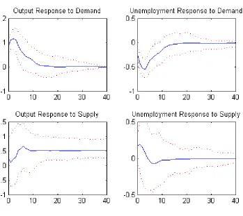
Blanchard and Quah (1989) consider a VAR model consisting of the real

GNP growth and unemployment rate. The demand and supply shocks are

identified by the assumption that the demand shock has no long-run effects

on the output level. GNP data are quarterly while the unemployment data

are monthly. In their paper, “the monthly unemployment data are averaged

to provide quarterly observations” (p. 661). We use data of the same sample

period (1950:2 to 1987:4) and follow their methods to filter the data and

remove the effects of trend and structural breaks. The only difference is that

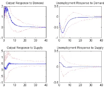
we mix quarterly GNP growth and monthly unemployment rate, allowing for

16 lags.6 _{Once the parameters are estimated, the VARDAS model becomes}

a standard VAR model and the structural shocks can be identified with the

long-run constraint without modification. The responses of output and

un-employment to the demand and supply shocks are plotted in Figure 2. For

comparison, the results of a Bayesian version of the quarterly data VAR are

shown in Figure 1, which is essentially a replication of Blanchard and Quah

(1989). Note that in their paper the confidence interval is based on one

stan-dard deviation, while we plot the Bayesian 95% credible interval with highest

posterior density (HPD). The dynamic patterns are consistent with those in

the original paper but the HPD bands are narrower, which demonstrates

efficiency gains due to making full use of the monthly unemployment data.

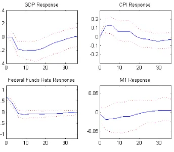
The second application is a structural VAR model with short-run

restric-tions. Christiano et al. (1998) propose a block diagonal recursiveness

assump-tion to identify monetary policy shocks. The variables in the VAR system are

6

Estimation with 8, 12, 24 lags produces little difference in the shape of the impulse

classified into three groups. The second group consists of only one monetary

policy instrument, whose innovations reflect monetary policy shocks. The

identification assumption is that the policy instrument has no

contempora-neous effect on the variables in the first group, and the third group has no

contemporaneous effect on the previous two groups. This assumption enables

a partial identification of monetary shocks by cholesky decomposition,

leav-ing other shocks unidentified. We put GDP and the CPI in the first group,

federal funds rate (FF) as the policy instrument and the money stock M1 in

the third group. Monthly data of the CPI, FF and M1 are available while

GDP data are quarterly. The sample period is chosen as 1974:01 to 2006:12

since there might be structural breaks before and after that time interval.

Data are Hodrick-Prescott filtered for we are interested in the cyclical

com-ponent of the data. There is a tradeoff between richer dynamics with more

lags and harder estimation with more parameters. In a four-variable VAR,

an additional lag means 16 more parameters. We allow 4 lags in the

quar-terly data VAR (by averaging the monthly data other than GDP) and 6 lags

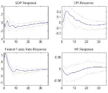
in the monthly VARDAS model. Impulse response functions using quarterly

data are reported in Figure 3 and the results with mixed data are plotted in

Figure 4. Unlike the case of long-run identification, Figure 3 and 4 are not

directly comparable in that the short-run identification constraints, though

in the same format, should be interpreted differently. In the quarterly data

VAR, to identify the monetary shocks we require monetary shocks have no

effects, so there are grounds for believing Figure 4 presents a more reliable

dynamic picture on how the economy responds to monetary shocks. This

is a major advantage of the VARDAS model in structural shocks

identifica-tion with short-run economic constraints. After a contracidentifica-tionary monetary

shock, GDP and M1 react negatively as expected, but the CPI rises steadily,

a phenomenon long documented in the literature as the price puzzle (Sims,

1992; Eichenbaum, 1992). Christiano et al. (1998) suggest including an index

of sensitive commodity prices can resolve the anomaly, a topic beyond the

Figure 1: The dynamic effects of demand and supply shocks with the quarterly GNP

growth and quarterly unemployment data. The solid line plots the posterior mean of the

impulse-response function and the dotted lines are the 95% HPD credible bands. Figure

Figure 2: The dynamic effects of demand and supply shocks with the quarterly GNP

growth and monthly unemployment data. The solid line plots the posterior mean of the

impulse-response function and the dotted lines are the 95% HPD credible bands. It is

estimated by the monthly VARDAS model, but the unit of the horizontal axis is adjusted

Figure 3: The dynamic effects of monetary policy shocks with the quarterly data. The

identification constraints are monetary shocks have no contemporaneous effects on the

Figure 4: The dynamic effects of monetary policy shocks with the monthly data except

for quarterly GDP, estimated by the VARDAS model. The identification constraints are

monetary shocks have no contemporaneous effects on the output and price in a month. The solid line plots the posterior mean of the impulse-response function and the dotted

7. Conclusion

The structural VAR model has been fruitfully applied in macroeconomics

to unveil the dynamic paths of economic variables responding to nominal or

real shocks. Such an analysis involves two stages in general. The first stage

is to estimate a reduced-form VAR model and invert to its moving

aver-age representation. In the second staver-age, restrictions are imposed to identify

structural shocks so as to conduct impulse response analysis. The second

stage embodies scientific insights of the macroeconomists and is

undoubt-edly the core of the VAR analysis, while the first stage is largely statistical

and mechanical. However, a better estimate of the reduced-form VAR model

translates to a more accurate impulse-response curve, and thus presents a

more transparent picture of dynamic relations in the macroeconomy. The

VARDAS model only operates on the first stage. Varied frequency data

are reconciled neither in an aggregated model by averaging nor in a

disag-gregated model by imputation. They are harmonized in one Bayesian model

that makes full use of the available information to sample the latent variables.

Technical details aside, the VARDAS approach just provides a more precise

estimate of the model parameters, leaving intact the economic insights that

hallmark the structural VAR analysis.

Amemiya, T., Wu, R. Y., 1972. The effect of aggregation on prediction in

the autoregressive model. Journal of the American Statistical Association

67 (339), 628–632.

Andreou, E., Ghysels, E., Kourtellos, A., 2010. Regression models with mixed

Aruoba, S. B.and Diebold, F. X., Scotti, C., 2009. Real-time measurement

of business conditions. Journal of Business & Economic Statistics 27 (4),

417–427.

Blanchard, O. J., Quah, D., 1989. The dynamic effects of aggregate demand

and supply disturbances. American Economic Review 79 (4), 655–73.

Breitung, J., Swanson, N., 2002. Temporal aggregation and spurious

instan-taneous causality in multiple time series models. Journal of Time Series

Analysis 23 (6), 651–665.

Camacho, M., Perez-Quiros, G., 2010. Introducing the euro-sting: Short-term

indicator of euro area growth. Journal of Applied Econometrics 25 (4),

663–694.

Chen, B., Zadrozny, P., 1998. An extended yule-walker method for estimating

a vector autoregressive model with mixed-frequency data. In: NBER/NSF

Time Series Conference.

Chiu, C., Eraker, B., Foerster, A., Kim, T. B., Seoane, H., 2011. Estimating

var sampled at mixed or irregular spaced frequencies: A bayesian approach

(manuscript).

Christiano, L. J., Eichenbaum, M., Evans, C. L., 1998. Monetary policy

shocks: What have we learned and to what end? (6400).

Clements, M. P., Galvao, A. B., 2008. Macroeconomic forecasting with

mixed-frequency data. Journal of Business and Economic Statistics 26,

Clements, M. P., Galvao, A. B., 2009. Forecasting us output growth using

leading indicators: an appraisal using midas models. Journal of Applied

Econometrics 24 (7), 1187–1206.

Eichenbaum, M., 1992. Comment on interpreting the macroeconomic time

series facts : The effects of monetary policy. European Economic Review

36 (5), 1001–1011.

Ghysels, E., Santa-Clara, P., Valkanov, R., 2006. Predicting volatility:

get-ting the most out of return data sampled at different frequencies. Journal

of Econometrics 131 (1-2), 59–95.

Ghysels, E., Sinko, A., Valkanov, R., 2007. Midas regressions: Further results

and new directions. Econometric Reviews 26 (1), 53–90.

Hyung, N., Granger, C. W., 2008. Linking series generated at different

fre-quencies. Journal of Forecasting 27 (2), 95–108.

Kuzin, V., Marcellino, M., Schumacher, C., 2011. Midas vs. mixed-frequency

var: Nowcasting gdp in the euro area. International Journal of Forecasting

27 (2), 529–542.

Marcellino, M., 1999. Some consequences of temporal aggregation in

empir-ical analysis. Journal of Business & Economic Statistics 17 (1), 129–136.

Marcellino, M., Schumacher, C., 2010. Factor midas for nowcasting and

fore-casting with ragged-edge data: A model comparison for german gdp.

Mariano, R. S., Murasawa, Y., 2003. A new coincident index of business

cycles based on monthly and quarterly series. Journal of Applied

Econo-metrics 18 (4), 427–443.

Mariano, R. S., Murasawa, Y., 2010. A coincident index, common factors,

and monthly real gdp. Oxford Bulletin of Economics and Statistics 72 (1),

27–46.

Mittnik, S., Zadrozny, P. A., 2004. Forecasting quarterly german gdp at

monthly intervals using monthly ifo business conditions data.

Silvestrini, A., Veredas, D., 2008. Temporal aggregation of univariate and

multivariate time series models: A survey. Journal of Economic Surveys

22 (3), 458–497.

Sims, C. A., 1980. Macroeconomics and reality. Econometrica 48 (1), 1–48.

Sims, C. A., 1992. Interpreting the macroeconomic time series facts: The

effects of monetary policy. European Economic Review 36 (5), 975–1000.

Tiao, G. C., 1972. Asymptotic behaviour of temporal aggregates of time

series. Biometrika 59 (3), 525–531.

Tiao, G. C., Wei, W. S., 1976. Effect of temporal aggregation on the dynamic

relationship of two time series variables. Biometrika 63 (3), pp. 513–523.

Zadrozny, P., 1988. Gaussian likelihood of continuous-time armax models

when data are stocks and flows at different frequencies. Econometric