The Rectangle Rule for Computing Cauchy Principal Value Integral on Circle

http://dx.doi.org/10.4236/ajcm.2016.62011

The Rectangle Rule for Computing Cauchy

Principal Value Integral on Circle

Jin Li1,2_{, Benxue Gong}3_{, Wei Liu}4

1_{School of Science, Shandong Jianzhu University, Jinan, China} 2_{School of Mathematics, Shandong University, Jinan, China} 3_{School of Science, Shandong University of Technology, Zibo, China}

4_{School of Mathematics and Statistics Science, Ludong University, Yantai, China}

Received 8 March 2016; accepted 10 June 2016; published 13 June 2016 Copyright © 2016 by authors and Scientific Research Publishing Inc.

This work is licensed under the Creative Commons Attribution International License (CC BY). http://creativecommons.org/licenses/by/4.0/

Abstract

The classical composite rectangle (constant) rule for the computation of Cauchy principle value

integral with the singular kernel cotx s

2

− _{is discussed. We show that the superconvergence rate}

of the composite midpoint rule occurs at certain local coodinate of each subinterval and obtain the corresponding superconvergence error estimate. Then collation methods are presented to solve certain kind of Hilbert singular integral equation. At last, some numerical examples are provided to validate the theoretical analysis.

Keywords

Cauchy Principal Value Integral, Extrapolation Method, Composite Rectangle Rule, Superconvergence, Error Expansion

1. Introduction

Consider the Cauchy principle integral

(

)

2π

( )

( )

(

)

; cot d , 0, 2π

2

c c

x s

I f s =

∫

+ − f x x=g s s∈ (1)

where c 2π

c

+

∫

denotes a Cauchy principle value integral and s is the singular point.

( )

( )

( )

2π 2π

0 0

cot d lim cot d cot d ,

2 2 2

c s

c s

x s x s x s

f x x ε f x x _ε f x x

ε

+ −

+ →

− ₌  − ₊ − 

 



∫



∫

∫

(2)

Cauchy principal value integrals have recently attracted a lot of attention [1]-[5]. The main reason for this interest is probably due to the fact that integral equations with Cauchy principal value integrals have shown to be an adequate tool for the modeling of many physical situations, such as acoustics, fluid mechanics, elasticity, fracture mechanics and electromagnetic scattering problems and so on. It is the aim of this paper to investigate the superconvergence phenomenon of rectangle rule for it and, in particular, to derive error estimates.

The superconvergence of composite Newton-Cotes rules for Hadamard finite-part integrals was studied in [6]-

[8], where the superconvergence rate and the superconvergence point were presented, respectively. Lyness [9]

derived the Euler-Maclaurin formula for Cauchy principal value integrals. Elliott and Venturino [2] employed sigmoidal transformations to obtain better approximation to Cauchy principal value integrals. In the reference Avram Sidi [10][11] and [12] presented high-accuracy numerical quadrature methods for integrals of singular periodic functions. The classical Euler-Maclaurin summation formula [13] expressed the difference between a definite integral over

[ ]

0,1 and its approximation using the trapezoidal rule with step length h=1m as an asymptotic expansion in powers of h together with a remainder term.

The extrapolation method for the computation of Hadamard finite-part integrals on the interval and in a circle is studied in [14] and [15] which focus on the asymptotic expansion of error function. Based on the asymptotic expansion of the error functional, algorithm with theoretical analysis of the generalized extrapolation is given.

In this paper, the density function f(x) is replaced by the approximation function fC(x) while the singular kernel

cot 2 x−s

is computed analysis in each subinterval, where fC(x) is the midpoint rectangle rule. This methods

may be considered as the semi-discrete methods and the order of singularity kernel can be reduced somehow. This idea was firstly presented by Linz [16] in the paper to calculated the hypersingular integral on interval. He used the trapezoidal rule and Simpson rule to approximate the density function f(x) and the convergence rate was

( )

k , 1, 2

O h k= when the singular point was always located at the middle of certain subinterval. This paper

focuses on the superconvergence of mid-rectangle rule for Cauchy principle integrals. We prove both theoreti- cally and numerically that the composite mid-rectangle rule reaches the superconvergence rate when the local coordinate of the singular point s is ±1. Then a collation methods is presented to solve certain kind of Hilbert singular integral equation.

The rest of this paper is organized as follows. In Sect. 2, after introducing some basic formulas of the rectangle rule, we present the main resluts. In Sect. 3, we perform the proof. Finally, several numerical examples are provided to validate our analysis.

2. Main Result

Let c=x0<x1<<xn−1<xn= +c 2π be a uniform partition of the interval

[

c c, +2π

]

with mesh size 2π

h= n. Define by fC

( )

x the piecewise constant interpolant for f x

( )

( )

( )

ˆ , ˆ 1 , 1, 2, ,

2

C j j j

h

f x = f x x =x₋ + j=  n (3)

and a linear transformation

( ) (

)

(

1

)

[ ]

ˆj : 1 j j 2 j, 1,1 ,

x=x τ = τ+ x+ −x +x τ∈ − (4)

from the reference element

[

−1,1

]

to the subinterval x xj, j+1. Replacing f x

( )

in (2) with fC

( )

x gives

the composite rectangle rule:

(

)

2π

( )

( )

( )

(

)

(

)

1

ˆ

; : cot d ; , ,

2

n c

n _c j j n

i

x s

I f s + f x x ω s f x I f s E f s

=

−

=

_∫

=

∑

= − (5)

where En

(

f s,

)

denotes the error functional and ωi

( )

s is the Cote coefficients given by

( )

cot ˆ .

2 j j

x s s h

We also define

(

)

cot , ,

( ) 2

2, .

s

x s

x s x s

k x

x s −

 − ≠

 = 

 ₌



(7)

Theorem 1: Assume f x

( )

∈C c c1

[

, +2π

]

. For the rectangle rule I_n

(

f s,

)

defined as (5). Assume that

(

1

)

2

m

s=x + +τ h , there exist a positive constant C, independent of h and s, such that

(

,

)

(

ln ln

( )

)

,

n

E f s ≤C h+ γ τ h (8)

where

( )

0

1

min .

2 j j n

s x

h

τ γ τ

≤ ≤

− −

= = (9)

Proof: Let R x

( )

= f x

( )

− fC

( )

x , then we have R x

( )

≤Ch. As

(

)

( )

(

)

( )

( )

( )

_{( )}

2π 2π

2π 2π

, cot d

2

2 cot d

2

2

2 d d

c n _c c c

c c _s

c c

x s

E f s R x x

R x

x s

x s x

x s

R x k x

x R x x

x s x s

+ +

+ +

− =

−

= −

− −

= +

− −

∫

∫

∫

∫

(10)

For the first part of (10), we have

( )

(

)(

)

(

)(

)

( )

(

)

1

1

1 _2π

0,

1

1 1

d d d

2π ln

ln ln

i m

i m

n _{x x c}

x c x

i i m

m m

R x

x Ch x x

x s s x x s

c s s c

Ch

x s s x

C h γ τ h

+

+

− ₊

= ≠

+

 

≤ _ + _

−  − − 

+ − −

=

− −

≤ +

∑ ∫

∫

∫

(11)

For the second part of (10),

( )

( )

( )

_{( )}

_{( )}

1 1 1

d ln ln

m m

m m

x x

m

x x

m

R x R x R s x s

x R s Ch

x s x s s x γ τ

+ + − ₊ −

≤ + ≤

− − −

∫

∫

(12)

( )

_{( )}

( )

_{( )}

2π 2 2π 2

d d ln .

c _s c _s

c c

k x k x

R x x Ch x Ch

x s x s γ τ

+ − + −

≤ ≤

− −

∫

∫

(13)

Combining (11) and (13) together, the proof is completed. Setting

( )

1

1

,

ˆ

cot cot d , ,

2 2

ˆ

cot cot d , .

2 2

m

m

j

i

x _m

x n j

x j

x

x s

x s

x j m

I s

x s

x s

x j m

+

+

  − ₋ −  ₌

 _ _



=  _{ − }

−

 _{ −  ≠}

 _{ }



∫

∫

(14)

Lemma 1: Assume s=x_m+ +

(

τ 1

)

h 2 with τ∈ −

[

1,1

]

. Let In j,

( )

s be defined by (14), then there holds

that

( )

(

(

)

(

)

)

(

)

, 1 1

1 1

1

ˆ

cos cos sin

n j j j j

k k

I s k x s k x s h k x s

k

∞ ∞

+ +

= =

=

∑

− − − −

∑

− (15)

( )

(

1

)

,

0

1 ˆ

lim cot cot d

2 2

ˆ

2 ln 2 sin 2 ln 2 sin cot

2 2 2

m

m

s x _m

n m _{x s}

m m m

x s x s

I s x

x s x s x s

h ε ε ε + − + → + − −   = + _ − _   − − −       = _{ }− _{ }− _{ }      

∫

∫

(16)

For i≠m, taking integration by parts on the correspondent Riemann integral, we have

( )

1

,

ˆ

2 ln 2 sin 2 ln 2 sin cot

2 2 2

i i i

n i

x s x s x s

I s = _ − _− _ + − _−h_ − _

      (17)

Now, by using the well-known identity

1

1

ln 2 sin cos

2 n x nx n ∞ =

= −

∑

(18)

and

1

1

cot sin

2 2 n

x

nx

∞ =

=

∑

(19)

The proof is completed. By the identity in [17]

1

π cot π ,

l l x x l =∞ =−∞ = +

∑

(20)

then we get

1 1

2 2 2

cot

2 l 2π l 2π

x s

x s x s l x s l

∞ ∞

= =

− _{= + +}

−

∑

− −

∑

− + (21)

and

(

)

(

)(

)

(

(

)(

)

)

(

)

(

)(

)

1 1 1 1 1 1

ˆ 2 2 2

cot cot

2 2 2π 2π

2 2 2

ˆ ˆ 2π ˆ 2π

ˆ ˆ

2 2

ˆ 2π ˆ 2π

ˆ 2

ˆ

2π 2π

m

l l

l l

m m m

m m l m m m l m x s x s

x s x s l x s l

x s x s l x s l

x x x x

x s x s x s l x s l

x x

x s l x s l

∞ ∞ = = ∞ ∞ = = ∞ = ∞ = − − − = + + − − − − +   −_ + + _ − − − − +   − − = + − − − − − − − + − + − +

∑

∑

∑

∑

∑

∑

(22)

For j=m, by the definition of cauchy principal value integral, we have

( )

(

)

(

)

(

)

(

)(

)

(

)

(

)(

)

(

)

(

)(

)

1 1 1 1 , 0 0 1 1 ˆ

lim cot cot d

2 2 ˆ 2 lim d ˆ ˆ 2 d ˆ

2π 2π

ˆ 2

d . ˆ

2π 2π

m m m m m m m m

s x _m

n m _{x s}

s x _m x s m x _m x l m x _m x l m x s x s

I s x

x x

x

x s x s

x x

x

x s l x s l

x x

x

x s l x s l

ε ε ε ε ε ε + + + + − + → − + → ∞ = ∞ = − −   = + _ − _   − = + − − − + − − − − − + − + − +

∫

∫

∫

∫

∑∫

∑∫

(23)

Let Qn

( )

x be the function of the second kind associated with the Legendre polynomial P xn

( )

, defined by

( )

( )

( )

0 1 0

1 1

ln , 1.

2 1

x

Q x Q x xQ x

x +

= = −

− (24)

We also define

(

)

( )

(

)

(

)

(

)

0

, : 2 2 , 1,1 .

i

W f τ f τ f i τ f i τ τ

∞ =

= +

∑

_ + + − + _ ∈ − (25)

Then, by the definition of W,

( )( )

0

1

1 1 1 2 1 2 1

ln ln ln

2 1 2 2 1 2 1

1 2 1

lim ln 0,

2 2 1

i i

i i

W Q

i i

i i

τ τ τ

τ

τ τ τ

τ τ

∞ = →∞

+  + + − − 

= + _ + _

−  − + + − 

+ +

= =

+ −

∑

(

)( )

(

)

(

)

(

)

0 2 2 2

1

2 2

1 2 1 2 1

π 1

1 1 π

lim tan ,

1

2 2 2

2 2

i

k n

n

k n

i i

W xQ

i i

k

τ τ τ

τ

τ τ τ

τ τ

∞

= = →∞ =−

 _{+ − +} 

′ = −  + 

 

− _ + − − + − _

+

= = −

+ +

∑

∑

it follows that

(

0 0

)

(

)

π 1

, π tan .

2

W Q +xQ′τ = − τ+ (26)

Theorem 2: Assume

( )

2l

[

, 2π

]

f x ∈C c c+ . For the rectangle rule In

(

f s defined as ,

)

(5). Assume that

(

1

)

2

m

s=x + +τ h , there exist a positive constant C, independent of h and s, such that

(

)

( )

π

(

1

)

( )

, π tan ,

2

n n

E f s = −f s τ+ + s (27)

where

( )

_max

{

( )

}

(

_{ln ln}

( )

)

2l

n s ≤C ks x h+ γ τ h

 (28)

( )

γ τ is defined as (9).

It is known that the global convergence rate of the composite rectangle rule is lower than Riemann integral.

3. Proof of the Theorem

In this section, we study the superconvergence of the composite rectangle rule for Cauchy principle integrals.

Preliminaries

In the following analysis, C will denote a generic constant that is independent of h and s and it may have different values in different places.

Lemma 2: Under the same assumptions of Theorem 2, it holds that

( )

( )

( )

( )

( ) ( )

(

)

( )

_{( )}

( ) (

)

( )

_{( )}

( )

(

)

2 1 1

2 2

2 2

1 2

ˆ

cot cot

2 2

ˆ

cot cot

2 2

ˆ ˆ

cot cot

! 2 2

ˆ ˆ

cot cot .

2 ! 2 2 ! 2

j C j

i

l _i

i j

j i

l l

l

l j

j

x s

x s

f x f x

x s

x s

f s

x s

f s x s

x s x s

i

x s

f s x s f s

x s x s

l l

− =

−

− ₋

−

 − 

=_ − _

 

−

 − 

+ _ − − − _

 

− −

+ − − −

where s1∈

( )

x s sˆ ,j , 2∈

( )

x s, .

Proof: Performing Taylor expansion of fC

( )

x at the point x, we have

( )

( )

2 1 ( )

( )

(

)

( )

_{( )}

2

( )

(

)

₂ 1

1

ˆ

ˆ ˆ ˆ cot

! 2 ! 2

i l

l _{i l}

j

C j j j

i

x s

f s f s

f x f s x s x s

i l

− =

−

= +

∑

− + − (29)

and

( )

( )

2 1 ( )

( ) ( )

( )

_{( ) (}

2

( )

)

2 2

1

cot .

! 2 ! 2

i l

l

i l

i

f s f s x s

f x f s x s x s

i l

− =

−

= +

∑

− + − (30)

Combining (29) and (30) together we get the results. Proof of Theorem 2: we have

(

)

( )

( )

( )

( )

( )

( )

_{( )}

(

)

1 1 1 1 1 2π 0, 1 0, 1 0,

2 1 1

1 0,

cot d cot

2 2

ˆ

ˆ

cot cot d

2 2

ˆ

cot cot d

2 2

ˆ ˆ

cot cot

! 2 2

m m j j j j j j n

x c _j

j

c x

j j m

n _x

j

j x

j j m

n _x

j x

j j m

i

l n _x

i j

x

i j j m

x s x s

f x x h f x

x s x s

f x f x x

x s x s

f s x

x s

f s x s

x s x

i + + + + − + = ≠ − = ≠ − = ≠ − − = = ≠ − − + − −  −  = _ − _   −  −  = _ − _   − − + − −

∑

∫

∫

∑ ∫

∑ ∫

∑

∑ ∫

(

)

( )

_{( )}

( ) (

)

( )

_{( )}

( )

(

)

1 2 2 1 ₂ 2 1 2 0, d ˆ ˆ

cot cot d .

2 ! 2 2 ! 2

j

j

i j

l l

n _{x l}

l j

j x

j j m

s x

x s

f s x s f s

x s x s x

l l + − = ≠   −      − −  +  − − −     

∑ ∫

(31)

For i=m, we have

( )

( )

( )

( )

( )

(

)

(

)

( )

_{( )}

( ) (

)

( )

_{( )}

( )

(

)

1 1 1 1 1 2 1 1 2 2 2 2 1 2 ˆ ˆ ˆ ˆ

cot d cot cot cot d

2 2 2 2

ˆ ˆ

ˆ

cot cot d cot cot d

2 2 2 2

ˆ ˆ

cot cot

2 ! 2 2 !

m m m m m m m m m m

x _m x _m

m m

x x

l

x m x i m i

m x x i l l l x l j x

x s x s

x s x s

f x x h f x f x f x x

x s x s

x s x s

f s x x s x s x

f s x s f s

x s x s

l l + + + + + − = − − − − − = − − − − −     = _ − _ + _ − − − _     − + − − −

∑∫

∫

∫

∫

∫

d 2 j x s x  −        (32)

Putting (31) and (32) together yields

( )

( )

( )

( )

( )

( )

_{( )}

(

)

(

)

( ) ( )

1 1 1 1 2π 0 1 0 1 0 1 1 0, 0 ˆ ˆ

cot d cot

2 2

ˆ

ˆ

cot cot d

2 2

ˆ

cot cot d

2 2

ˆ ˆ

cot cot d

! 2 2

j j j j j j n c j j c j n x j j x j n _x j x j i _n i

x i j

j x

i j j m

i

x s

x s

f x x h f x

x s

x s

f x f x x

x s

x s

f s x

x s

f s x s

x s x s x

i

S τ f s

+ + + − + = − = − = ∞ − = = ≠ = − − ₋ −  −  = _ − _   −  −  = _ − _   −  −  + _ − − − _   = +

∑

∑∫

∑∫

∑ ∫

∫

∑

( )

_{( )}

(

)

(

)

( )

_{( )}

( ) (

)

( )

_{( )}

( )

(

)

1 1

2 1 1

1 0 2 2 1 ₂ 2 1 2 0 ˆ ˆ

cot cot d

! 2 2

ˆ ˆ

cot cot d .

2 ! 2 2 ! 2

j

j

j

j

i

l n _{x i}

i j j x

j

l l

n _{x l}

l j

j x

j

x s

f s x s

x s x s x

i

x s

f s x s f s

x s x s x

Here

( )

1 1

0

0

ˆ

cot cot d

2 2

j

j

n _x

j x

j

x s

x s

S τ + x

− =

−

 − 

= _ − _

 

∑∫

with the linear transformation from tj−1,tj to the identity interval

[

−1,1

]

. As for the last part of

(

)

(

)

1

1 0

ˆ ˆ

cot cot d

2 2

j

j

n _i

x i j

j x

j

x s

x s

x s x s x

+

− =

−

 − _{− − −} 

 

 

∑∫

which can be considered as the error estimate of left rectangle rule for the definite integral b

(

)

i 1d , 2

a t s t i

−

− ≥

∫

.

Obviously,by the Theorem, it can be expanded by the Euler-Maclaurin expansions and we have

(

)

(

)

1

( ) ( )

( 1)

₍

₎

( 1)

1

, d , 1

!

b i k k k

i k

n _a

k

B

E f h t s t b s a s h k i

k

θ

∞

− − −

=

 

=

_∫

− +

∑

_ − − − _ ≤ − (34)

It is easy to see that there are not relation with the singular point

s

which can be written as

(

)

(

)

1

1

, b i d , 1.

i k

n _a k

k

E f h t s t c h k i

∞ −

=

=

_∫

− +

∑

≤ − (35)

The proof is complete. 

We actually obtain the error expansion of the rectangle rule and moreover, get the explicit expression of the first order term. So it is easy for us to get the superconvergence point with S0

( )

τ =0, which means that

1

τ = ± is the superconvergence point in subinterval not near the end of the interval. Based on the theorem 1, we present the modify rectangle rule

(

;

)

(

;

)

( )

π tanπ

(

1

)

.

2

n n

I f s =I f s −f s τ+ (36)

4. Numerical Example

In this section, computational results are reported.

Example 1: We consider the Hilbert singular integral with f x

( )

=cosx+sinx c=0. [ ]n4

(

1

)

2

s= +c x + +τ h with τ = ±1 is the superconvergence point.

From Table 1 and Table 2, we know that the superconvergence point is ±1 with the coordinate location of singular point equal zero, while for the local coordinate of singular point do not equal zero,it is not convergence in general which coincides with our analysis.

For the modify classical rectangle rule, from Table 3 and Table 4, for the non-superconvergence point and the supersonvergence point, we all get the supercocergence phenomenon.

In this section, we consider the integral equation

( )

( )

(

)

2π 0 1

cot d , 0, 2π ,

2π 2

x s

f x − x=g s s∈

∫

(37)

with the compatibility condition

( )

2π

0 g x dx=0.

∫

(38)

As in [5], under the condition of (38), there exists a unique solution for the integral Equation (37). In order to get a unique solution, we adopt the following condition

( )

2π

0 f x dx=0.

∫

(39)

By choosing the middle points xˆk =xk−1+h2

(

k=1, 2,,n

)

, we get the composite rectangle rule In

(

f s;

)

to approximate the Hilbert singular integral in (37), then the following linear system is obtained

( )

1

ˆ 1

ˆ

cot , 1, 2, , ,

2 n

m k

m k

m

x x

h f g x k n

π =

−

  _{= =}

 

 

Table 1. An error estimate of the rectangle rule s=x_{[ ]n4} +

(

τ+1

)

h 2.

1

τ= τ= −1 2

3

τ = 1

2

τ =

8 −1.7764e−015 0 6.6963e−001 1.7335e+000

16 −1.7764e−015 0 2.2690e+000 4.1887e+000

32 0 0 2.9882e+000 5.2932e+000

64 −5.3291e−015 2.6645e−015 3.3190e+000 5.8039e+000

128 −4.4409e−014 −4.3521e−014 3.4762e+000 6.0477e+000

256 1.3323e−014 −9.7700e−015 3.5526e+000 6.1665e+000

Table 2. An error estimate of the rectangle rule s=x₀+

(

τ+1

)

h2.

1

τ= τ= −1 2

3

τ = 1

2

τ =

8 −1.1102e−015 −6.2172e−015 5.0863e+000 8.7150e+000

16 −3.1086e−015 −7.1054e−015 4.6011e+000 7.8365e+000

32 −8.8818e−015 −4.3521e−014 4.1701e+000 7.1371e+000

64 −2.6645e−015 −1.7764e−014 3.9119e+000 6.7284e+000

128 −2.6645e−015 −3.8192e−014 3.7729e+000 6.5102e+000

[image:8.595.93.540.42.740.2]

256 2.9310e−014 1.0658e−013 3.7010e+000 6.3978e+000

Table 3. An error estimate of the modify rectangle rule s=x_{[ ]n4} +

(

τ+1

)

h2.

1

τ= τ= −1 2

3

τ = 1

2

τ =

8 −1.7764e−015 0 −1.7764e−015 3.5527e−015

16 −1.7764e−015 0 −5.3291e−015 7.1054e−015

32 0 0 −3.5527e−015 2.3093e−014

64 −5.3291e−015 2.6645e−015 1.0658e−014 3.0198e−014

128 −4.4409e−014 −4.3521e−014 −4.7962e−014 −1.3323e−013

256 1.3323e−014 −9.7700e−015 −6.0396e−014 2.8422e−014

Table 4. An error estimate of the modify rectangle rule s=x₀+

(

τ+1

)

h2.

1

τ= τ= −1 2

3

τ = 1

2

τ =

8 −1.1102e−015 −6.2172e−015 −8.8818e−016 0

16 −3.1086e−015 −7.1054e−015 −2.8866e−015 −3.5527e−015

32 −8.8818e−015 −4.3521e−014 −9.5479e−015 −1.5099e−014

64 −2.6645e−015 −1.7764e−014 −7.3275e−015 −3.6637e−015

128 −2.6645e−015 −3.8192e−014 4.4409e−015 −2.6645e−014

and written as the matrix expression as

,

a e

n n n

A F =G (41)

where

( )

(

)

T

(

( ) ( )

( )

)

T

1 2 1 2

, ˆ 1

cot , , 1, 2, , ,

π 2

ˆ ˆ ˆ

, , , , , , , ,

n km n n j k km

a e

n n n n

A a

x x

a h k m n

F f f f G g x g x g x

×

=

−

 

= _{ } =

 

= =



 

(42)

here fk

(

k=1, 2,,n

)

denotes the numerical solution of f at xˆk. By directly calculation, we get An that is not only a symmetric Toeplitz matrix but also a circulant matrix. As for any k=1, 2,,n,

1 1

ˆ 1

cot 0,

π 2

n n

m k

km

m m

x x

a h

= =

−

 

= _{ }=

 

∑

∑

(43)

from (43), we know that An is singular matrix, then we cannot use system (40) or (41) to solve the integral Equation (37).

In order to get a well-conditioned definite system, we introduce a regularizing factor γ0n in (40), which leads to linear system

( )

0

1

1

ˆ 1

ˆ

cot ,

π 2

0, n

m k

n m k

m n

m m

x x

h f g x

f

γ

=

=

 ₊  −  ₌

  

  



 ₌



∑

∑

(44)

where γ_0n defined by

( )

0

1

1

ˆ .

2π

n

n k

k

g x h

γ

=

=

∑

(45)

Then the matrix form of system (44) can be presented as

1 1 1,

a e n n n

A+F+ =G+ (46)

where

T

0

1 1 1

0 0

, a n , e ,

n

n n a n e

n n

n n

e

A F G

F G

e A

γ

+ + +

     

=  =  = 

   

  (47)

and

T

1,1, ,1

n

n

e =  _

 .

Example 2: Now we consider an example of solving Hilbert integral equation by collocation scheme. Let

( )

cos sin

g s = s− s, the exact solution is f x

( )

=cosx+sinx. We examine the maximal nodal error, defined by

( )

1

min _{i i} ,

i n

e_∞ f x f

≤ ≤

= − (48)

where f ii

(

=1, 2,,n

)

denotes the approximation of f x

( )

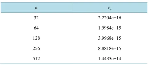
at xˆi. Numerical results presented in Table 5 show that both the maximal nodal errors are as follow.

Acknowledgements

[image:10.595.191.437.108.216.2]

Table 5.Errors for the solution of the Hilbert integral equation of

first kind.

n e∞

32 2.2204e−16

64 1.9984e−15

128 3.9968e−15

256 8.8818e−15

512 1.4433e−14

Grant No. 11101247), China Postdoctoral Science Foundation (Grant No. 2013M540541 and 2015T80703). The work of Wei Liu was supported by National Natural Science Foundation of China (Grant No. 11401289).

References

[1] Diethdm, K. (1995) Asymptotically Sharp Error Bounds for a Quadrature Rule for Cauchy Principal Value Integrals Based on Piecewise Linear Interpolation, Approx. Theory of Probability and Its Applications, 11, 78-89.

[2] Elliott, D. and Venturino, E. (1997) Sigmoidal Transformations and the Euler-Maclaurin Expansion for Evaluating Certain Hadamard Finite-Part Integrals. Numerische Mathematik, 77, 453-465.

http://dx.doi.org/10.1007/s002110050295

[3] Hasegawa, T. (2004) Uniform Approximations to Finite Hilbert Transform and Its Derivative. Journal of Computa-tional and Applied Mathematics, 163, 127-138. http://dx.doi.org/10.1016/j.cam.2003.08.059

[4] Ioakimidis, N.I. (1985) On the Uniform Convergence of Gaussian Quadrature Rules for Cauchy Principal Value Inte-grals and Their Derivatives. Mathematics of Computation, 44, 191-198.

http://dx.doi.org/10.1090/S0025-5718-1985-0771040-8

[5] Yu, D.H. (2002) Natural Boundary Integrals Method and Its Applications. Kluwer Academic Publishers, Dordrecht, 50.

[6] Yu, D.H. (1992) The Approximate Computation of Hypersingular Integrals on Interval. Numerical Mathematics: A Journal of Chinese Universities (English Series), 1, 114-127.

[7] Zhang, X.P., Wu, J.M. and Yu, D.H. (2010) The Superconvergence of Composite Trapezoidal Rule for Hadamard Fi-nite-Part Integral on a Circle and Its Application. International Journal of Computer Mathematics, 87, 855-876. http://dx.doi.org/10.1080/00207160802226517

[8] Wu, J.M. and Sun, W.W. (2008) The Superconvergence of Newton-Cotes Rules for the Hadamard Finite-Part Integral on an Interval. Numerische Mathematik, 109, 143-165. http://dx.doi.org/10.1007/s00211-007-0125-7

[9] Lyness, J.N. and Ninhan, B.W. (1967) Numerical Quadrature and Asymptotic Expansions. Mathematics of Computa-tion, 21, 162-178. http://dx.doi.org/10.1090/S0025-5718-1967-0225488-X

[10] Sidi, A. and Israeli, M. (1988) Quadrature Methods for Periodic Singular and Weakly Singular Fredholm Integral Equ-ations. Journal of Scientific Computing, 3, 201-231. http://dx.doi.org/10.1007/BF01061258

[11] Sidi, A. (2003) Practical Extrapolation Methods: Theory and Applications. Cambridge University Press, Cambridge. http://dx.doi.org/10.1017/CBO9780511546815

[12] Zeng, G., Lei, L. and Huang, J. (2015) A New Construction of Quadrature Formulas for Cauchy Singular Integral.

Journal of Computational Analysis and Applications, 17, 426-436.

[13] Sidi, A. (2014) Analysis of Errors in Some Recent Numerical Quadrature Formulas for Periodic Singular and Hyper-singular Integrals via Regularization. Applied Numerical Mathematics, 81, 30-39.

http://dx.doi.org/10.1016/j.apnum.2014.02.011

[14] Li, J., Wu, J.M. and Yu, D.H. (2009) Generalized Extrapolation for Computation of Hypersingular Integrals in Boun-dary Element Methods. CMES: Computer Modeling in Engineering & Sciences, 42, 151-175.

[15] Li, J., Zhang, X.P. and Yu, D.H. (2013) Extrapolation Methods to Compute Hypersingular Integral in Boundary Ele-ment Methods. Science China Mathematics, 56, 1647-1660. http://dx.doi.org/10.1007/s11425-013-4593-1

[16] Linz, P. (1985) On the Approximate Computation of Certain Strongly Singular Integrals. Computing, 35, 345-353. http://dx.doi.org/10.1007/BF02240199