Dynamic Econometric Testing of Climate Change and of its Causes

Munich Personal RePEc Archive

Dynamic Econometric Testing of Climate

Change and of its Causes

Travaglini, Guido

Università degli Studi di Roma "La Sapienza"

30 June 2010

Dynamic Econometric Testing of Climate Change and of its Causes

Guido Travaglini Istituto di Economia e Finanza Università di Roma “La Sapienza”

Email: [email protected] June 30, 2010.

Fully revised and updated version of the paper No.669 presented at the EEA-ESEM Congress, Milan, August 27-31, 2008.

Keywords: Generalized Method of Moments, Global Warming, Principal Component and Factor Analysis, Structural Breaks.

Abstract

1. Introduction

This paper combines several aspects of modern econometric methods: Structural Breaks Analysis (SBA), Principal Component Analysis (PCA), estimation by the Generalized Method of Moments (GMM), instrument validity and coefficient hypothesis testing in the presence of weak instruments or weak identification (WI). In particular, it develops a novel SBA method to detect level and trend breaks of time series occurring at unknown dates, it introduces a recent method based on PCA and Principal Factor Analysis (PFA) to select the true forcing regressors (henceforth defined as forcings) within a large dataset, and it utilizes several recent procedures to assess instrument validity in a context characterized by (possible) weakness and nonexogeneity.

Specifically, this composite methodology is employed at different stages of an econometric analysis of climate-related natural and anthropogenic variables that run from 1850 to present. The purpose of this methodology is to perform a series of tests regarding the timely behavior of world average temperatures during that period: the possibility of structural breaks, which is a test of the hypothesis of any significant climate change that may have occurred at some date in the past, the taxonomy of its forcings and in particular the role of anthropogenic variables, the validity (exogeneity and relevance) of the instruments utilized, the Wald-type hypothesis testing of estimated coefficients in the presence of weakness and, finally, time-varying coefficients and PCA shares of the forcings.

The plan of the paper is the following. Section 2 formulates the theoretical null and alternative hypotheses of the proposed SBA testing procedure, and empirically computes its corresponding critical values by producing their finite-sample Monte Carlo (MC) simulations. Appendix 1 contains some related off-text material on this account.

Section 3 synthetically explains the characteristics and properties of the GMM (Hansen, 1982), a classical toolkit of Instrumental Variables (IV) estimation necessary to circumvent problems arising from errors in variables, endogeneity and omitted variables. Parametric and nonparametric tests for selecting the ‘best’ GMM model specification among alternative sizes of the instrument and regressor sets, even in the presence of WI, are introduced and explained. Finally, its dynamic counterpart is briefly examined and a procedure for computing time-varying PCA and significance-weighted shares is introduced. Appendix 2 contains some basic information regarding the PCA and PFA procedures utilized to compute the true number of factors.

Section 4 is addressed at testing a red-hot topic that represents the center stage of many recent top-level discussions: the phenomenon known as ‘Global Warming’ (GW) and its anthropogenic origin, supposedly determined by the rapid pace of industrialization and the ensuing worldwide development of productive and commercial activities. The time series of world average temperatures and of a large set of human and natural forcings for the period 1850-2006 are introduced and then filtered by means of the Hodrick-Prescott (HP) procedure. After selection of the ‘best’ GMM model specification, dynamic GMM estimation results producing the time series of the regression coefficients, their t statistics and the significance-weighted shares are obtained and further examined.

Section 5 concludes by showing that there exist no significant breaks in world temperatures and that anthropogenic forcings play no role in climate changes which are instead attributable to Pacific Decadal Oscillations, sunspots and intense volcanic activity.

2. Structural Breaks Analysis (SBA)

multiple structural breaks of unknown date (Banerjee et al., 1992; Bai and Perron, 2003; Perron and Zhu, 2005; Perron and Yabu, 2009, Kim and Perron, 2009).

2.1. Testing for Structural Breaks: the Null and the Alternative Hypotheses

By drawing from this vast and knowledgeable experience, and especially from a chief contribution in the field (Perron and Zhu, 2005), a novel t-statistic testing procedure for multiple level and trend breaks occurring at unknown dates (Vogelsang, 1997) is here proposed. This procedure is easy and fast at identifying break dates, as it compares the critical t statistic, obtained by MC simulation under the null hypothesis of a time series with stationary noise, with the actual t statistic obtained under the alternative represented by a time-series model with a constant, a trend term, the two structural breaks and one or more stationary noise components.

The departing point to test for the existence of structural breaks in a time series function is the null hypothesis given by the series with I(0) errors, namely

1)

∆ ≡

y

_t

y

_t

−

y

_t−1

=

e

_t

where

y

_t is nonstationary and spans the period t∈

[

1,T

]

, and e_t ∼I I D. . .(0,σ2) _{corresponds to a} standard Data Generating Process (DGP) with draws from a random normal distribution whose underlying true process is a driftless random walk.

Let the field of fractional real numbers be Λ =

{

λ

₀,1−

λ

₀

}

, where

0

<

λ

₀

<

1

is the preselect trimming factor, normally required to avoid endpoint spurious estimation in the presence of unknown-date breaks (Andrews, 1993). Let the true break fraction be λ∈ Λ for

0 0

0

<

λ

<

λ

<

(1

−

λ

)

and

λ

₀T ≤

λ

T ≤(1−

λ

₀)T the field of integers wherein the true break date occurs.

Given the null hypothesis of eq. (1), the simplest available alternative is provided by a series with a constant and a trend, their respective breaks, and a time vector of noise. Specifically, the alternative is represented by an augmented AO model (Perron, 1997), usually estimated by Ordinary Least Squares (OLS). In Sect. 3.1, the alternative will be augmented with a vector of exogenous I(0) series and estimated by GMM in order to account for heteroskedasticity, autocorrelation and endogeneity.

Formally, the alternative specification of eq. (1) is represented by a extension of the null that includes a set of deterministic variables, namely, a constant, a linear trend and their corresponding SB dummies. The result is

2)

∆ =

y

_t

µ λ

₁

( )

+

µ λ

₂

( )

DU

_t

( )

λ

+

τ λ

₁

( )

t

+

τ λ

₂

( )

DT

_t

( )

λ

+

ε λ

_t

( );

∀ ∈ Λ

λ

where the

λ

notation refers to the time-changing coefficients and variables of the dynamic equation estimation.

The disturbance

ε λ

t

( )

=

I I D

. . .(0,

σ

2

)

is I(0) with

E

(

ε

t

( ) '

λ

ε

s

( )

λ

)

=

0;

∀

t s

,

,

s

≠

t

(Perron and Zhu, 2005; Perron and Yabu, 2009). Thus, eq. (2) is expected to be stationary and to exhibit no autocorrelation.

Specifically, the two differently defined unknown-date break dummies included in eq. (2)

t

DU

and

DT

_t are defined as follows:

B)

DT

_t

=

(

t

−

TB

_t

)1(

t

>

TB

_t

)

, a change in the trend slope (

τ

₁−

τ

₀), namely a change in the inclination of

∆

y

_t around the deterministic time trend.

By stacking for

t

∈

[

1,

T

]

both dummy series, we obtain the following

T T

×

matrices:

DU

=

0 1 1 ... 1

0 0 1 ... 1

... ... ... ... ...

0 0 0 ... 1

 

 

 

 

 

 

,

DT

=

0 1 2 ... 1

0 0 1 ... 2

... ... ... ... ...

0 0 0 ...

T

T

T T

−

 

 

−

 

 

 

−

 

where each row of

DU

and

DT

respectively represents

DU

_t and

DT

_t,

∀ ∈

t

[1, ]

T

. The trimming factor, usually set to 10-15%, is made compulsory by the existence of zeros in both matrices that causes spurious regression estimates. Theoretically, since unknown-date structural breaks are a nuisance in regression analysis (this is not the case of standard dummies), endpoint loss of power against alternatives occurs (Andrews, 1993) because of the trailing zeros in DU and DT. In practice, however, the endpoint cuts can be asymmetric and endogenously computed by simply detecting the length of both trailing zero sets. Fortunately enough, in most cases, the trimming factor is found to be much shorter at the end of the sample, thereby letting room for the inclusion and evaluation of more recent data. For expositional simplicity, however, the notation

λ

₀ valid for both endpoints is retained in the present context.

The coefficients

µ

₀ and

τ

₀ are the respective pre-change values. As a general rule there follows, from the above notation, that any of the two structural breaks is represented by a vector of integers

∀

TB

_t

∈

{

λ

₀

T

, (1

−

λ

₀

)

T

}

(Banerjee et al., 1992). From eqs. (1) and (2),

E

(

∆

y

_t

)

≡

0

and

(

1 0

,

1 0

)

( )

0

E

µ − µ τ − τ

λ =

, that is, breaks in mean and in trend slope are a temporary phenomenon. Therefore, case A corresponds to unknown-date structural breaks in terms of temporary change(s) in the level of the endogenous variable (the "crash" model). Similarly, case B corresponds to temporary shifts in its trend slope (the "changing growth" model) (Perron 1997; Banerjee et al., 1992; Vogelsang and Perron, 1998). Eq. (2), by using both cases together, is defined by Perron and Zhu (2005) as a “local disjoint broken trend” model with I(0) errors (their “Model IIb”).

In addition, for

E

(

∆

y

_t

)

≡

0

in eq. (2),

E

(

µ λ τ λ ≠

₁

( ), ( )

₁

)

0

, i.e. the coefficients are expected not to equal zero. Appendix 1 demonstrates that

β

₀ holds only for a non-breaks alternative model, namely, when

λ =

1

. If this is not the case, i.e. when time series are characterized by a broken trend, both breaks are likely to occur.

As usual in the break literature, eq. (2) is estimated sequentially for all

λ

∈ Λ

. After dropping the

λ

notation for ease of reading from the single coefficients, we obtain a time series of

length

1 (1

+

−

λ

₀

)

T

of the coefficient vector

β λ

ˆ( )

≡

[

µ µ τ τ

₁

,

₂

, ,

_{1 2}

]

which is closely akin to the Kalman filter ‘changing coefficients’ procedure. As a by-product, the t statistics of

β λ

ˆ ( )

for the

same trimmed interval are obtained and defined as

t

ˆ ( )

_µ

λ

_t and

t

ˆ ( )

_τ

λ

_t, respectively. They are nonstandard-distributed since the corresponding breaks are associated to unknown dates and thus appear as a nuisance in eq. (2), (Andrews, 1993; Vogelsang, 1999).

weighted average is achieved and tested for (e.g. Andrews, 1993), all that is required is to sequentially find as many t statistics that exceed in absolute terms the appropriately tabulated critical value for a preselect magnitude of

λ

.

In practice, after producing the critical values for different magnitudes of

λ

by MC simulation, respectively denoted as

t

_T

( , )

λ

L

and

t

_T

( , )

λ

T

, any

n

≥

1

occurrence for a given

confidence level (e.g. 95%) whereby

t

ˆ ( )

_µ

λ

_t

>

t

_T

( , )

λ

L

and

t

ˆ ( )

_τ

λ

_t

>

t

_T

( , )

λ

T

indicates the

existence of

n

≥

1

level and trend breaks, respectively, just as with standard t-statistic testing1.

2.2. Theoretical and Finite-sample Critical t _Statistics

To achieve the above-stated goal, some additional notation is required. Let the

K

₁-sized

vector of the deterministic variables of eq. (2) be specified as

X

_t

=

[

1, ,

t DU

_t

( ),

λ

DT

_t

( )

λ

]

, and let the Ordinary Least Squares (OLS) estimated coefficient vector be

3)

0 0

0 0

(1 ) (1 )

ˆ( ) '

T T

t t t t

t T t

y X X X

λ λ λ λ β λ − − = = =

∑

∆

∑

with variance

0 1 0 1 (1 ) 2 I ' T

K t t

t X X λ λ

σ

− − =    



∑

 , where

I

K1 is the

K

1

×

K

1 identity matrix. Let also the

estimated and the true parameter vectors be formally defined as

β λ

ˆ

( )

≡

[

µ τ µ τ

ˆ ˆ ˆ

₁

, ,

_{1 2}

,

ˆ

₂

]

andβ* ≡_µ τ µ τ₁*, ₁*, ₂*, ₂*_, respectively, such that the scaling matrix of the different rates of

convergence of

β λ

ˆ ( )

with respect to

β

* is given by 1/ 2 3/ 2 1/ 2 3/2

, , ,

t diag T T T T 

ϒ = _{ } which ensures

the asymptotics of the estimated parameters.

Then, by generating

∆

y

_t according to eq. (1) we have, for

0

<

λ

<

1

4) ˆ( ) *

(

( )

)

1 ( )

L

T β λ β T λ T λ

−

 

ϒ _ − _ → Θ Ψ ,

whereby, for W r( ) a standard Brownian motion in the plane r∈[0,1], the following expressions ensue:

5)

1 1

0 0

( ) (1), (1) ( ) , (1 ) (1), (1 ) (1) ( )

T λ σ W W W r dr λ W λ W W r dr

  

Ψ =  − − −  − 

   

∫

∫

 and 6) 2 2 3 2 3 (1 ) 1 1 / 2 1

2

(1 ) (2 3 )

1 / 3

2 6 ( ) (1 ) 1 2 (1 ) 3 T λ λ

λ λ λ

λ λ λ λ  ₋  −     − − +    

Θ = 

−   −     −       .

7)

(

)

₍

₎

(

)

2 2

3 2 3

* 2 2 2 2 3 3

4 6 2 6

12 6 12

0

0

ˆ( ) N , _{4 2 1}

0 6

1 1

0

3 3 1

12 1

T

λ λ λ λ

λ λ λ

β λ β σ _λ

λ λ λ λ

λ λ λ λ    −          _{− −}  _{   }      

ϒ _ − _{   − }

     − ₋        _{− +}      _{ − }   ∼

where the square matrix corresponds to

(

Θ

_T

( )

λ

)

−1.

The corresponding asymptotic t statistics of the coefficient vector for testing the null

hypothesis that

β λ

ˆ

( )

−

β

*

=

0

are computed as follows:

8)

(

)

1

(

)

1/2

( ) ( ) ( ) ( )

T T T T

t λ = Θ λ − Ψ λ Ω λ

where T

( )

λ

σ

2

I

₄

(

T

( )

λ

)

1

−

Ω

=

Θ

. The ensuing theoretical t statistic values regarding the level break

( , )

T

t

λ

L

and the trend break

t

_T

( , )

λ

T

are thus

8.1)

[

]

1

0 1/ 2

(1) ( )

( , ) 3

(1 )

T

W W r dr

t L λ λ λ λ − = −

∫

8.2) 1

1/ 2 0

1/ 2 2

(3 1) (1) 2(2 1) ( )

( , ) 3

(1 )(3 3 1)

T

W W r dr

t T

λ λ λ

λ

λ λ λ λ

− − − =  _{− − +}   

∫

while the other two non-break statistics are reported in Appendix 1. The empirical critical values of the above-shown t statistics are obtained by MC simulation of the values of the null provided by eq. (1)2. For select magnitudes of

λ

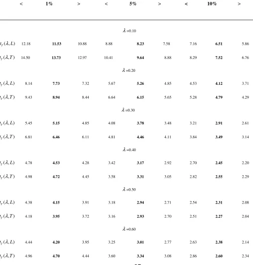
running from 0.10 to 0.90, and for a reasonable sample size (T = 200), the 1%, 5% and 10% finite-sample absolute critical values of eqs. (8.1) and (8.2) are reported in Table 1 together with their 10% upper and lower confidence bands.

The critical values, after selecting the sample size and the number of draws (N=1,000), are obtained by means of the following steps:

(i) computing a T T× matrix of the standard Gaussian random variates

(

)

. . . 0, ,

j j

w ∼N I D ν T _where

(

_{0,1 ,}

)

[

_1,

]

j N j T

ν

∼ ∈ _;

(ii) computing each value of

e

_t in eq. (1) as the algebraic sum of each column of the random

variate matrix. Therefore

1 T t j j e w =

=

∑

is a T×1-sizedmatrix of artificial discrete realizations;

(iii) integrating

e

_t over the time span

t

=

1,...,

T

by computing the rolling partial sums of

e

_t and obtain the

T

×

1-sized

matrix of nonstationary series

y

_t;

(iv) exploiting the values

e

_t

and

y

_t−1 to approximate the scalar-sized Brownian functionals

1

0

(1) and ( )

W

∫

W r dr of eq. (5) with the corresponding discrete sums exhibited in Appendix 1;

From Table 1 the absolute critical values can be seen to achieve minimal absolutes at

λ

=0.50 and larger values at both ends of

λ

. Finally, except for

λ

=0.50,

t

_T

( , )

λ

L

is smaller than

( , )

T

t

λ

T

by a factor that reaches 1.2 at both ends4. In addition, the reported t statistics are nonstandard. In fact, though exhibiting zero mean, they have non-unit variances that strictly hinge on the values of

λ

and of

σ

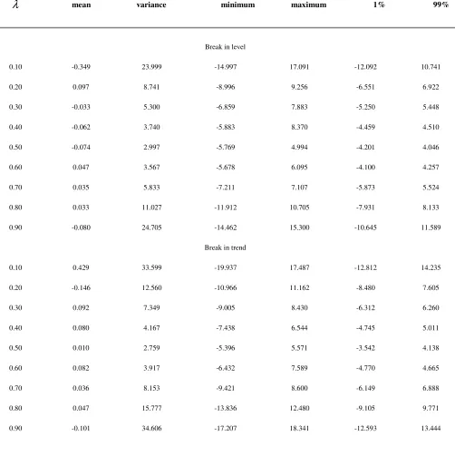
. As shown in Appendix 1, this is applicable also to the other two non-break statistics.

Descriptive statistics of the t statistic of a break in level, eq. (8.1), and of the t statistic of a break in trend, eq. (8.2) for 1,000 MC draws of eq. (1) for a sample size T=200 and break fractions

0.10

≤

λ

≤

0.90

are supplied in Table 2. As expected, the means hover around zero for any value of

λ

, while the variances attain a minimal value in correspondence of

λ

=0.50, where they share an almost equal value and then increase by eight and ten times at both ends, respectively. Specifically, the estimated variance of the first statistic is on average 40% smaller than the second, reflecting the similar gap in their critical values reported in Table 1. Similar gaps are recorded also for the extrema and for the 1% and 99% fractile values.

3. The Generalized Method of Moments (GMM)

The time series of length

1 (1

+

−

λ

₀

)

T

of the coefficients and of the t-statistics may be estimated sequentially by means of GMM which exhibits the following characteristics:

1) the model used by the GMM method perfectly suits eq. (2) so that the estimated relevant t

statistics are easily comparable to their simulated critical values of Table 1;

2) the estimated coefficients are scale-free relative to equations in levels as the regressors in origin are often differently indexed with the risk of producing, otherwise, spurious coefficient results;

3) the autocorrelation and heteroskedasticity of the error term are corrected for by using the Heteroskedasticity and Autocorrelation Consistent (HAC) covariance estimator (Newey and West, 1987);

4) By accordingly selecting the optimal instrument vector, GMM disposes of parameter inconsistency deriving from left-out variables, errors in variables (i.e. mismeasurement) and/or endogeneity.

In addition, the GMM method may be exploited to compute time-varying standard and significance-weighted PCA shares, a useful tool to assess the relevance of the regressors in determining the causative behavior of the endogenous variable. By including time changes in the parameters of eq. (2), the method is more properly defined as Dynamic GMM. This technique is described in detail in Sect. 3.2.

3.1. Properties ofthe GMM Estimator and Weak Instruments Robust Testing

Before delving into the dynamic version of the GMM method, some aspects of the static standard GMM estimation method must be introduced. GMM uses sample moments derived from first-stage (possibly consistent) IV estimation, usually Two-Stage Least Squares (TSLS). In turn, IV estimation requires an appropriate model setting where the major features tying the endogenous variable, the regressors and the instruments are explicitly formalized.

The departing point to construct the GMM model is represented by eq. (2) which, for ease of reading and of treatment, is simplified by removing the dynamic

λ

notation from therein in order to operate in a static environment. In addition, the

X

_t vector of deterministics of Sect. 2.2 may be made to include without any loss of generality, if desired, additional nondeterministic explanatory

variables. Consider a

K

₂-sized vector of stationary stochastic components

2

,1,..., ,_K

t t t

which extends the vector of regressors to a K-sized vector X_t ≡_X_t⋮Xɶ_t_{, where}

1 2

K =K +K .

Therefore, the IV setup is represented by a standard structural form and its reduced-form counterpart

9.1)

∆ =

y

_t

X

_t

β

+

e

_t

9.2)

X

_t

=

Z

_t

Π +

v

_t

where X :_t

(

T×K

)

is defined as above, Z_t:

(

T×L

)

is a matrix of

L

≥

K

instrumental variables,

(

)

: K 1

β

× and Π:

(

L K×

)

are a coefficient vector and matrix, respectively,

(

)

(

2

)

: 1 . . . 0,

t e

e T× ∼N I D σ _{and :}

(

)

_{. . . 0,}

(

)

t

v T×K ∼ N I D Σ _{are the disturbance terms, and}

(

X '

_{t t}

)

0

E

e

=

,

E e v

(

_t

'

_t

)

=

0

,

E X Z

(

_t

'

_t

)

≠

0

and finally

Π

is of full rank5.

The requirement of stationarity of eqs. (9.1) and (9.2) is crucial. In fact, nonstationary series unless cointegrated notoriously produce spurious coefficient t statistics, error autocorrelation and a

bloated

R

2 (Granger and Newbold, 1974; Phillips, 1986). Spuriousness is also found between series generated as independent stationary series with or without linear trends and with seasonality (Granger et al., 2001) or with structural breaks (Noriega and Ventosa-Santaulària, 2005). These occurrences are found in this literature with OLS regressions where the t statistics – in particular those of the deterministic components – diverge as the number of observations gets large6, although HAC-based correction methods are available (Sun, 2004).

In practice, the requirements that e_t =I I D. . .(0,σ_e2), E

(

e et' s

)

=0, t ≠s and also, given p a

preselect lag integer, 2

1

E 0

p t i i

e₋ =

 

=

 



∑

 for no heteroskedasticity must be met as from eq. (9.1). Tests to check for such occurrences are available in great numbers and kinds, e.g. the Durbin-Watson and the Breusch–Godfrey statistics, the ARCH test for heteroskedasticity, etc., and may be exploited to perform first-hand model selection. First differencing, centering-and-scaling and Hodrick-Prescott (HP) smoothed filtering (Hodrick and Prescott, 1997) are the major competitors addressed at performing the necessary data transformation to attain a stationary environment.

Recently, standard two-step GMM has undergone mounting criticism on accounts of parameter consistency and HAC optimal bandwidth selection in a small-sample setting, and especially in the presence of (many) WI (e.g. Newey and Smith, 2004; Sun et al., 2008; Newey and Windmeijer, 2009). It has been in fact demonstrated that the efficiency of the IV and of the GMM estimators can be improved by using a large instrument set at the cost – however – of heavy biases. This occurs especially in the presence of WI, which distorts standard parameter Wald-based test results culminating in the “weak IV asymptotics” in which the coefficient vector in the first-stage regression shrinks to zero as the sample size goes to infinity (Staiger and Stock, 1997; Stock and Wright, 2000; Andrews and Stock, 2007).

The Wald-type hypothesis testing considered is framed as the standard null, namely

H

₀

:

β

=

β

₀, where

β

₀ is some theoretical value, or the first-stage estimated coefficient

(

β

_TSLS

)

, or even zero for the entire K-sized coefficient vector or for an R-sized subset

thereof

(

1≤R<K

)

. In the presence of WI such tests are found to be heavily distorted and characterized by low power. Moreover, in the many-WI case, GMM estimates are biased toward OLS estimates (Newey and Windmeijer, 2009), while the J test statistic of overidentifying restrictions (Hansen, 1982) has low power and produces spurious identification results (Kleibergen and Mavroeidis, 2009).

empirical cases a full set of strong instruments may be unavailable7. Elsewise, as Yogo correctly points out (2004), researchers may be still interested at parameter estimation even in the presence of a detected WI, and size-robust parameter tests for a given null hypothesis may be employed and confidence intervals (CI) may be constructed by “inversion” of the appropriately supplied non-Wald test statistics (Moreira, 2003; Cruz and Moreira, 2005; Andrews et al. 2006; Kleibergen, 2002, 2005, 2008; Kleibergen and Mavroeidis, 2009).

The tests proposed by the mentioned authors are intended to replace the traditional testing methodology that depends on nuisance parameters (e.g. the reduced-form coefficients of eq. (9.2)). To eliminate these effects, the mentioned authors have devised these novel test statistics that are pivotal, invariant and similar8 and thus have good size properties under both strong and WI, although not all have optimal power properties and in several cases CI might not even be constructed.

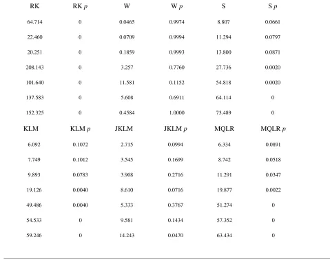
The proposed tests belong to the classes of the Anderson-Rubin (AR, Anderson and Rubin, 1949), of the score Lagrange Multiplier (LM) and of the Likelihood-Ratio (LR) test statistics. These tests originate in the field of IV estimation test (Stock and Wright, 2000; Stock et al., 2002; Stock and Yogo, 2003; Moreira, 2003) but have been recently extended to GMM (Kleibergen, 2005; Kleibergen and Mavroeidis, 2009). For ease of space, only these versions are reported in the present context, together with the corrected J test statistic for overidentification and the Jacobian rank statistic. They are denoted by the authors respectively as: S, KLM, MQLR, JKLM and RK, and fully described in Kleibergen (2005) and in Kleibergen and Mavroeidis (2009). Under the null they

are all distributed as a

χ

2 statistic with (L-K+R), R, R, (L-K) and (L-K) degrees of freedom, respectively.

The first three GMM-based statistics behave much as their IV counterparts and are similarly constructed, although with some specific differences (Kleibergen, 2005; Kleibergen and Mavroeidis, 2009). For instance, the S statistic is different from the AR test (Stock and Wright, 2000; Stock et al., 2002; Stock and Yogo, 2003) since it is represented by the value function of the Continuous Updating Estimator (CUE) (Hansen et al., 1996), but it shares with AR the asymptotic distribution which does not depend on nuisance parameters even when the instruments are arbitrarily weak. Therefore, S is pivotal and can be used for inference and for constructing valid confidence sets (i.e. CI) by inversion as with the AR statistic (Staiger and Stock, 1997). However, it has however low power under overidentification and is outperformed by KLM and MQLR, and especially by the latter (Andrews et al., 2006).

The KLM test relies on the independence between average moments and their first derivatives (the Jacobian matrix), since correlation among them is a major source of bias in conventional GMM estimates and test statistics (Newey and Smith, 2004; Kleibergen, 2005; Newey and Windmeijer, 2009)9. However, this test statistic exhibits a loss of power when the objective function is maximal and becomes spurious. It is also size-distorted when such correlation is high (Kleibergen and Mavroeidis, 2009).

MQLR is an extension of the Conditional LR test (Moreira, 2003), so defined because it is conditioned on a statistic that is complete and sufficient under the null hypothesis. MQLR has the desirable features of having size that is robust to many WI and near-optimal power properties with Gaussian errors, and dominates the power of both S and KLM (Andrews et al., 2006; Mikusheva, 2007). This occurs because MQLR supersedes the assumption of full-column rank of the Jacobian matrix (Sect. 3.1) and conditions the LR statistic on a matrix reduced-rank test (Kleibergen, 2005; Kleibergen and Paap, 2007).

and is different from Hansen’s J statistic, which is evaluated at the parameter estimate. It is given by S-KLM, namely, the difference between a value function and an asymptotically independent test of the validity of the moment conditions.

3.2. Parametric and Nonparametric Tests for the Selection of Alternative GMM Models

In addition to appropriate data filtering required to remove spuriousness, and to due consideration of the possible WI phenomenon, GMM modeling involves a large variety of choices regarding the size of the regressor and instrument sets (given

L

≥

K

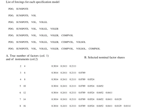
) and the magnitude of the bandwidth of the HAC weight matrix of eq. (16). Coefficient estimates and their efficiency and significance can in fact be very sensitive to different specification choices even with contiguous indicators (Hansen and West, 2002). Pretesting is thus necessary and (hopefully) sufficient to extract the “best” GMM model among different specifications, characterized each by different regressor and instrument vector sizes, HAC bandwidths and instrument strengths.

A complete although not exhaustive package of such pretest procedures contemplates three categories to be sequentially implemented for each select specification: true factor number and shares, first-stage tests, GMM tests. These categories constitute the following list:

A) True number of factors (Bai and Ng, 2002, 2007) and total number of instruments; B) Nominal factor shares;

C) First-stage tests for endogeneity: one-lag Granger causality F statistics running from structural residuals in eq. (9.1) to forcings and viceversa 10 (Granger, 1969);

D) First-stage WI tests for vector β₀ =0 in eq. (9.1): AR, LM, LR (Yogo, 2004);

E) First-stage relevance tests: minimum eigenvalues of the Concentration Parameter matrix and Cragg-Donald test statistic (Stock and Wright, 2000; Stock et al., 2002);

F) First-stage joint instrument exogeneity and relevance LR-type test (Kim and Lee, 2009); standard and asymptotic AR tests for overidentifying restrictions (Anatolyev and Gospodinov, 2010);

G) GMM standard J statistic (Hansen, 1982) and asymptotic J statistic (Imbens et al., 2003), both used to test the validity of the overidentifying restrictions;

H) GMM standard and asymptotic AR statistics tests for vectorβ₀ evaluated at the parameter estimate and validity of the overidentifying restrictions (Andrews and Stock, 2007);

I) GMM key statistics of the estimated residuals;

J) GMM coefficient vector and t statistics or WI-CI (e.g. Moreira, 2003; Cruz and Moreira, 2005; Kleibergen and Mavroeidis, 2009);

K) GMM Kleibergen’s tests for vectorβ0 =0, namely, the standard Wald test and RK, S, KLM, J

KLM and MQLR statistics described in Sect. 3.1.

The first category of pretesting (A and B) to be implemented is represented by the determination of the true number of regressors and of instruments in presence of a large dataset. It is a powerful alternative to traditional PCA methods utilized to compute the number of factors, (e.g. Anderson, 1984), which are shown by Bai and Ng (2002, 2008) not to produce consistent results as

,

T K → ∞.

This method is based on PFA and PCA, and is unanimously refered to as “factor modeling” or Factor IV (FIV) estimation. It can easily cope with many regressors without running into scarce degrees of freedom problems or in collinearity, and it is utilized to reduce in a first place the number of regressors, chosen among the widest possible available set, including variables that may be either justified or unjustified on theoretical grounds.

can be endogenously determined by formal statistical procedures characterized by information criteria, reported in Appendix 2, that place penalties on large datasets (Bai and Ng, 2002, 2007). The few and most relevant factors so obtained, in terms of computed shares, contain most of the model’s information and may be supplemented – if necessary – by additional regressors or instruments to form the entire available dataset.

The second category (C to F) includes first-stage testing of eqs. (9.1) and (9.2). They are well renowned in the current practitioner’s literature except for the last ones, which are of recent date. The first of these is denoted

Q

_IV by its authors (Kim and Lee, 2009), while the second is an

AR test adjusted for the number of instruments (Anatolyev and Gospodinov, 2010).

Q

_IV is a joint test for the IV instrument relevance and exogeneity with respect to structural errors, and is derived from two competing model specifications: one with exogenous and the other with irrelevant instruments. The

Q

_IV test is based on the LR of these two models; hence the joint null hypothesis

is

H

₀

:

β

=

0,

Π =

0

from eq. (9.1) and (9.2) respectively. In other words the null is represented by both exogeneity and irrelevance, and has a peculiar quasi

χ

2 distribution whose critical values are tabulated by the authors via MC simulation draws, although only for K ≤3regressors. If the

IV

Q

test statistic obtained from sample estimation rejects the null the instruments are deemed of good quality, and thus relevant, but not necessarily exactly exogenous.

The standard AR test statistic for overidentifying restrictions may be supplemented by a statistic bearing an asymptotic corrected size that prevents too frequent overrejections of the null hypothesis, determined by (moderately) many instruments. Anatolyev and Gospodinov (2010) found a similar occurrence with the standard J statistic, characterized by underrejection, and proposed an equivalent asymptotic test statistic. Both corrections build on foregoing work, where some authors have devised asymptotic corrected counterparts of the J and AR tests: the

2

ASY

J

L

J

L

−

=

and the

AR

_ASY

L

AR

1

L





=



−







tests, respectively distributed as

N

( )

0,1

and

(

0, 2

)

N

statistics (Imbens et al., 2003; Andrews and Stock, 2007).

Standard GMM-estimated residual statistics (category I) include the following: Standard Error (SE), Durbin-Watson statistic for first-order autocorrelation and ARCH test for heteroskedasticity (Engle, 1982), as well as the first-order autocorrelation coefficient that has been previously used as a selecting device for the appropriate data filtering (Sect. 3.1) and that can here perform a similar task on grounds of consistency.

3.3. The Dynamic GMM and the Construction of Dynamic Principal Components

Eq. (9.1) can be extended to produce the following dynamic estimating equation:

10)

∆ =

y

_t

X

_t

B

( ) '

λ

+

e

_t

( )

λ

where

1

1 2 1 2 1

( ) , , , , ,..., _K

B λ =_µ µ τ τ ξ ξ _ and

ξ

_k

,

k

=

1,...,

K

₂, are the coefficients of Xɶ_t, ∀λ ∈ Λ.

Finally, et( )λ =I I D. . .(0,σe2) and E X ( ) ' ( )

(

t

λ

et

λ

)

=0.

Eq. (10), just as eq. (2), enables constructing a time series of length

1 (1

+

−

λ

₀

)

T

of the

coefficient vector

B

( )

λ

and of the ensuing two t statistics

t

ˆ ( )

_µ

λ

_t and

t

ˆ ( )

_τ

λ

_t11. GMM estimation

other cases, and specifically when expectations are assumed to be the driving cause of the

behaviour of the endogenous variable (e.g. the Taylor Rule, Clarida et al., 2000), the vector

X

ɶ

_t is

augmented with its own leads and

K

₂ may be large. In such case, also the vector of instruments

Z

_t must be lengthened with the risk of producing, however, the many WI curse (Stock et al., 2002) for

L

→ ∞

, even if

T

→ ∞

.

The L-sized vector of sample moments, each being a random process of length

(

1−

λ

0

)

T, is

ˆ _ˆ

( , ) ( )

t t t

g

β λ

=Z ⊗e

λ

where the coefficient vector ˆβ and the first-stage residuals

e

ˆ

_t stem from a (possibly) consistent TSLS estimation of eq. (10). The sample means of the above are

(

)

(

)

0

(

)

0

(1 )

1

0

ˆ_{, 1} ˆ_,

T

t t T

g T g

λ

λ

β λ

λ

β λ

− −

=

=_ − _

∑

with the orthogonality property that E g_

(

β λ

ˆ,

)

_≡0, a necessary condition for instrument exogeneity. Let also the ensuing long-run p.d. weight matrix be

11)

(

)

0

0

(1 )

1 0

ˆ ˆ ˆ

( , ) : (1 ) ( , ) ( , ) '

T

t t

t T

W L L T g g

λ

λ

β λ

λ

β λ

β λ

− −

=

 

× =_ − _

∑

such that ˆ_GMM( ) arg min

(

g( , ) ( , )ˆ W ˆ 1g( , )ˆ

)

β

β

λ

β λ

β λ

−

β λ

∈Β

= .

Computation of the partial first derivatives of the sample moments yields the

KL L

×

Jacobian matrix 12) λ λ λ λ − − =   = _ − _

_∑

where

z

_t

,

x

_t respectively are the L.th and the K.th element of vectors Z_t and X_t. For relevance, we expect the Jacobian to be of full rank and no zero minimum Singular Value (SV). Finally the

efficient GMM estimator, by letting

0 0 (1 ) ' T t t t T

Z y z y

λ

λ −

=

=

∑

∆ , is

13) ˆ ˆ 1 1 ˆ 1

( ) '( ) ( , ) ( ) '( ) ( , ) '

GMM Gt W Gt Gt W Z yt

β

λ



λ

β λ

−

λ

−

λ

β λ

−

=_{ }

where, specifically

14)

1

1 2 1 2 1

ˆ

_{( )}

_{ˆ ˆ}

_,

_{, ,}

_{ˆ ˆ}

_{, ,...,}

ˆ

ˆ

GMM K

β

λ

=



_

µ µ τ τ ξ

ξ



_

whose asymptotic normality property is

1/2 ˆ ( ) * N 0, ( , )

(

ˆ

)

d GMM

T _β λ −β _ → S β λ

where

15) β λ _λ λ β λ − _λ λ −

− −

 

is the “sandwich” matrix.

In the presence of autocorrelation and/or heteroskedasticity of

e

_t

( )

λ

, that is, of persistence in the error term, the weight matrix of eq. (11) must be augmented in the form of the long-run covariance matrix

16)

0

0

(1 ) 1

(1 ) 1

ˆ

( , ) ( , ),

T

s T

s

W k s

b λ

λ

β λ λ

− −

=− − +

 

=  Γ

 

∑

where k is a preselect kernel function (e.g. Bartlett, Parzen, etc.), b is the bandwidth and

17)

0

0

(1 )

1

0 ˆ ˆ

( , ) (1 ) ( , ) ( , ) '

T

t s t t T

s T g g

λ

λ

λ λ β λ β λ

− −

+ =

 

Γ =_ − _

∑

is the s.th sample autocovariance of g_t( , )

β λ

ˆ ; s=0, 1,...± (Newey and West, 1987; Smith, 2005). Consistency of eq. (17) requires that (1−

λ

₀)T > >b 0 and that b→ ∞,

b

(1

−

λ

₀

)

T

→

0

as

T

→ ∞

i.e. that downweighting of

Γ

(

s

,

λ

)

operated by the smoother in eq. (16) be such as to produce a covariance matrix biased toward zero (Kiefer and Vogelsang, 2002). In common practice, the optimal value of b is (automatically) chosen to minimize the asymptotic mean square error of eq. (16).

Let X :t

(

T×K

)

as defined in Sect. 3.1. By virtue of the Spectral Decomposition Theorem,

define the symmetric asymptotic covariance matrix X 'X_{t t} Τ =ERE, where, for

[

1, ,

( ),

( )

]

t t t

X

=

t DU

λ

DT

λ

, X_t =_X_t⋮Xɶ_t_{ and}

1 2

K =K +K , Τ:

(

K×K

)

is a rate-of-convergence matrix with an upper left matrix

(

K1×K1

)

constituted by four 2 2× submatrices each containing

2 2 3 T T T T    

 , and 2 row and 2 column vectors

(

K2×1

)

of trailing

3 2

T placed in correspondence of

the time-related deterministics, that is, at K₁=2, 4. All other entries of matrix T are given by ones.

In addition, R is the

K

×

K

diagonal matrix of the eigenvalues ri,

(

i=1,...,K

)

in descending order, and E the same sized matrix of eigenvectors with column elements

(

)

E , _j j=1,...,K . We have

E

(

E'E

=

I

_K

)

, where

I

_K is the K×K identity matrix that ensures orthogonality of the principal component scores, which correspond to those in PFA (Appendix 2).

For each

E

_j, define the scalar η =j arg max E

( )

j , ( j≠i) such that the static PCA shares,

corresponding to the eigenvalues in descending order, are described as

18)

1

( | )

K

i i j i

i

s r r

=

= η

∑

where

(

r_i|η_j

)

denotes the association between the i.th eigenvalue and η_j.

After defining

α

_j the jth regressor’s marginal significance of the coefficient, the time series

of length

1 (1

+

−

λ

₀

)

T

of the jth regressor’s dynamic and significance-weighted share measured

over the trimmed interval t∈

{

λ

₀T, (1−

λ

₀)T

}

may be expressed as

19)

( )

( )

1

(1 ) ( | ) ;

K

i j i j i

i

s r r

=

 

λ =_ − α η _ λ ∀λ ∈ Λ



∑

 ,

where

(

1−αj

)

is the appropriate weight assigned to the ith share. Eq. (19) provides the dynamic

Apart from the dynamics involved, eq. (19) is preferable to eq. (18) because it weighs each component share by the statistical significance appended to its coefficient. Traditional PCA (e.g. Anderson, 1984), by ignoring this evidence and by sticking to nominal shares, may overstate in quite a few instances the components whose role is empirically found to be virtually close to zero. In alternative, the 1− α_j weight may be substituted for by the t statistic of the ith coefficient. The

advantage is represented by a ‘double weighting’ which includes also the absolute magnitude of the coefficient involved, and not only its standard error.

4. The Climate-related Dataset and the Empirical Estimations of Global Warming

In this Section all the climate-related data are exhibited together with an index of GW and then subjected, after appropriate filtering, to empirical estimation by dynamic GMM. Before proceeding, it is worth reminding the gaseous composition of Earth’s atmosphere: Nitrogen (

N

₂,

78%), Oxygen (

O

₂, 20%) and a few more, among which Carbon Dioxide (C

O

₂), Methane (C

H

₄),

Nitrous Oxide (

N

₂O) and Nitrogen Dioxide (N

O

₂). For ease of reading, the reported Mendeleyev symbols are respectively simplified as follows: N2, O2, CO2, CH4, N2O and NO2. Apart from water vapor, Chloro-Fluoro-Carbons (CFCs) and composite anthropogenic and natural aerosols, CO2, CH4 and NO2 purportedly reduce or trap the loss of Earth’s heat into space and cause – under certain conditions – the renowned “Greenhouse effect” and the consequential GW.

However, while GW is a minor part of the Earth’s long climatic history, other forcings at present and in the past times are held responsible of climate changes, although in many cases the data availability and affordability pose a restraint to large-scaled modeling addressed at event simulation, prediction or causative analysis. Precisely to this very end, the purpose of this Section is to introduce the available dataset and to perform such analysis for the sake of the advancement of knowledge.

4.1. Global Warming and Climate Forcings during the Period 1850-2006

Planet Earth has passed through many waxing and waning climate episodes during the entirety of its life. For instance, the Mid-Cretaceous (120-90 million years ago) and the Palaeocene Eocene Thermal Maximum (PETM, 55 million years ago) have experienced temperatures distinctly warmer than today, with animals and plants living at much higher latitudes and with higher carbon dioxide (CO2V) levels, roughly two to four times than the present-day ones.

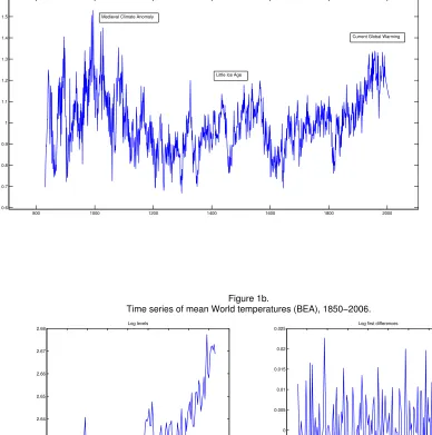
Abrupt climate changes have occurred also during the more recent Phanerozoic eon (Shaviv and Veizer, 2003), like the last glacial period (Alley, 2000), the Medieval Warm Period, centered around 1000 A.D., apparently the warmest period so far in the Christian era (Esper and Frank, 2009), and the Maunder Minimum in Europe during the years 1645-1715 A.D. Fig. 1a provides an account of the climatic oscillations that have occurred in the last twelve centuries or so, which are significantly proxied by the time series of the North Atlantic Ocean Mode (Trouet et al., 2009). Clearly, the Medieval Warm Period and the current GW represent the peaks, as found by other researchers too that use different proxies (Bürger, 2007).

While the above cited may be casual episodes of the often perverse relationship between humans and nature, the by now secular GW phenomenon, more recently dubbed “climate change” by the majority of its mentors, is undoubtedly cause of concern. In fact, the last hundred years or so have experienced a renewed climate change after the Maunder Minimum by exhibiting a rise in the mean global surface temperature by about 0.6 ± 0.2°C since the late 19th century, and by about 0.35 ±0.05° C over the last 40 years (Chenet et al., 2005). This phenomenon, while not unique in Earth’s history (Baliunas and Soon, 2003) as shown in Fig. 1a, has spurred intense debate on the analysis of its causes and is by now a worldwide major issue which involves popular media, scientists, corporations, governments and political organizations.

In fact, while the rise in temperatures is of undisputed evidence, yet at a slower pace in the last decade, the search for a main culprit is still in progress and well alive, and is being characterized by two opposing fronts regarding its causes: the advocates and the skeptics of its anthropogenic origin. Either sides hold on to their own positions since a decade or more and recent scuffles, such as the “Climategate” affair and the “hockey-stick” controversy demonstrate the vitality of the confrontation.

Advocates of the human-induced greenhouse effects, purportedly caused by CO2 emissions and industrial aerosols, include several scientists (e.g. Hansen et al., 2007), the UN-mandated Nobel-prized Intergovernmental Panel on Climate Change (IPCC) and large sections of governments and politicians12.

Skeptics, on the other hand, form a scientifically-based consensus that supports and proves the prevalence of long-run evolving natural causes, defined as “global forcings”, like solar activity (Abdussamatov, 2004), Cosmic Ray Flux (CRF) (Shaviv and Veizer, 2003; Svensmark, 1998; Bard and Frank, 2006, Usoskin et al., 2003), volcanic aerosols (Mann et al., 2005) and ocean currents (Gray et al., 1997). This consensus builds on reliable paleoclimatological dataset reconstructions (e.g. Crowley, 2000; Lean, 2000, 2004; Usoskin et al, 2003, 2004a, 2004b; Mann et al., 2005; Krivova et al., 2007), most of which are downloadable from the National Oceanic and Atmospheric Administration (NOAA) website.

The consensus share going to either group is not undisputed: according to a recent research (Doran and Zimmerman, 2009) the large-public opinion of Americans goes fifty/fifty, while more than 75% of peer-reviewed academic research papers backs the view that Earth's climate is affected by human activities. Other more recent sources of different origin express only little consensus on the anthropogenic causes of GW, and this has certainly dominated the choices made at the last IPCC Conference held in Copenhagen, December 2009.

One thing, however, stands clear to almost anybody: the analysis of the interaction of the variables implied in the secular GW process is very complex, as it requires countless and valuable in-depth experimenting stemming from different scientific fields, such as astrophysics, climatology, biology and chemistry. Statistics and econometrics may contribute to the current state of knowledge by supplying interesting insights into causality occurring in a casual environment. Not much work has been produced hitherto in this field, except for few though valuable contributions (e.g. Lanne and Liski, 2004; Kaufmann et al., 2006). Certainly more will come in the future.

GW is identifiable with data sets on land and sea temperature recordings collected by different agencies for select periods, areas, altitudes, hemispheres, etc. The Best Estimated Anomaly (BEA) of the updated HADCRUT3 dataset (Brohan et al., 2006), available for the period 1850-2006 on an annual basis, was selected due both to its space and time breadth. Therefore, the BEA index represents the endogenous variable used in eq. (10), whose GMM estimated parameter vector is given by eq. (14).

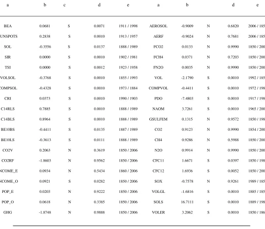
anthropogenic and natural forcings. Their tally is 37, of which 14 of anthropogenic origin and the others of natural or mixed origin.

The anthropogenic forcings include average real GDP percapita of the total 12 Western Europe major countries and of its overseas offshoots (U.S.A., Canada, Australia and New Zealand), and their total population (Maddison, 2007)14. They are respectively labeled INCOME_E, INCOME_O, POP_E and POP_O. Anthropogenic forcings also include the components of trace or greenhouse gases (GHG) that characterize air pollution. They are given by four measures of emissions: carbon dioxide (CO2) expressed in terms of global volume, which includes emissions from fossil-fuel burning, cement manufacture, and gas flaring (Marland et al., 2007), and final emissions of CO2, methane (CH4) and nitrous oxide (N2O), expressed in terms of Radiative Forcing (RF) measured in Watts per square meter (W/m2) (Robertson et al., 2001). Global sulphur emissions, expressed in thousands of metric tons, are also available (Stern, 2002). These forcings are respectively labeled as: CO2V, FCO2, FCH4, FN2O and GSULFEM. While the first and the last variable may be considered as a stock, the other three are a flow.

Needless to say, a part of the CO2-based emissions derive from the Global (oceans and land) Carbon Cycle, whose emissions and suspension in the atmosphere absorb radiation emitted from the Earth, trapping heat and contributing to GW, but at the same time shield the Earth from the Sun’s radiation, volcanic and geothermal activity, large forests, and man-made fermentation processes (e.g. beer and whiskey). Similarly, a part of CH4-based emissions derive from natural decay present in wetlands (e.g. swamps and marshes), urban landfills and waste treatment, livestock, volcanic activity, etc. Mostly man-made are instead N2O-based emissions deriving from internal combustion of engines, rocket motors, aerosol spray propellants, as well as analgesic & anesthetic products.

The category of natural forcings includes measures related to solar, volcanic and combined activities, as well as to cosmic rays and oceanic modes. As far as solar activity is concerned, there are 9 indicators: the average yearly number of monthly sunspot series (NGDC, 2007), a measure of total solar irradiance received at the outer surface of Earth's atmosphere in terms of RF (Krivova et al., 2007), tropical solar RF (Mann et al., 2005), composite solar RF, composite volcanic RF, and a total of four measures of Beryllium 10 (BE10) and Radiocarbon 14 (C14) that proxy solar RF (Crowley, 2000). In sequence, these forcings are labeled as: SUNSPOTS, SOL, SIR, TSI, COMPSOL, C14RLS, C14BLS, BE10BS and BE10LS.

Volcanic activity is represented by tropical and composite volcanic RF (Mann et al., 2005), and by a binary index that dates the major tropical eruptions (Ammann and Naveau, 2003), while oceanic modes are represented by Pacific Decadal Oscillations (Shen et al., 2006) and the North Atlantic Ocean Mode (Trouet et al., 2009). They are sequentially labeled as: VOL, COMPVOL, VOLER, PDO and NAOM. In addition, cosmic ray activity is proxied by the CRI flux (Usoskin et al., 2003; Alanko-Huotari et al., 2006), while the combined effects of volcanic and solar activities are proxied by the RF of the VOLSOL indicator (Mann et al., 2005). Natural and anthropogenic combined effects in the form of tropospheric aerosols are represented by sulphur and fossil-fuel black carbon emissions in volume and in RF (Crowley, 2000), respectively labeled as AEROSOL and AERF.

Finally, a climate-related valuable database (Stern, 2002, 2004) is added. It includes several indicators of human and natural origin, mostly adjusted variants of above-listed forcings. These are the world total sulphur emissions expressed in megatons, labeled as GSULFEM, and the radiative forcings from carbon dioxide, methane, nitrous oxide, two measures of chlorofluorocarbons responsible for ozone depletion, anthropogenic sulphur emissions, and two measures of volcanic and solar activities, respectively. All these variables are labelled as: CO2, CH4, N2O, CFC11, CFC12, SOX, VOLGL and SOLS.

anthropogenic forcings and volcanic activity, expressed in terms of their volatility coefficients. Also, the CO2-based and some anthropogenic forcings appear to be nonstationary as revealed by the p-values of the ADF t-test statistics. Oddly enough, BEA reveals stationarity, a feature confirmed also by other findings (fn. 15).

Thereafter, all level forcings – logged when applicable15 – are made to undergo appropriate HP filtering (excluding VOLER which is a dummy) and their cyclical components are extracted for the purposes of empirical estimation. The smoothing parameter chosen for the entire dataset is 6.25 as suggested by Ravn and Uhlig (2001). The rationale for this choice is based on the ARCH and autocorrelation coefficient results of the pretesting conducted on the structural equation (9.1) along the lines suggested in Sect. 3.1.

Therefore, alternative specifications of the equation include different sizes of the vector of forcings (K), ranging from a minimum of two to a maximum of eight true factors selected from the 37 forcings available (Bai and Ng, 2002, 2007, 2008), and of the instruments, whose size is chosen in all cases to be L=2K. For each specification, larger HP smoothing parameters (100 and 400), first differencing, and centering and scaling have also been applied to all variables. The latter alternatives, however, produced unsatisfactory or less satisfactory results and were therefore dismissed as candidates for data transformation16.

Fig. 1b illustrates the levels and the HP-filtered values of the logs of BEA and of all forcings. From the left panel, GW can be shown to exhibit a trending behavior since 185017, which is ostensibly stationary when appropriately filtered. The human forcings exhibit a trend, but methane (FCH4) seems to taper off in the last decade. On the other hand, the natural forcings are mostly cyclical, with SUNSPOTS exhibiting a known regularity of around 11 years. While retaining their labels, all of the variables used in calculations and estimations that will follow are henceforth understood, unless otherwise defined, to be represented by their HP-filtered magnitudes (see fn. 12).

4.2. Expected Effects of Forcings over Global Warming

The 37 listed forcings by means of ongoing research are expected to bear specific effects over the World temperature changes represented by BEA. Of the human forcings, economic activity and the size of population (INCOME and POPULATION) are expected to raise BEA via GHG emissions, extensive deforestation and generalized use of inefficient technologies. The United States and China nowadays appear by some estimates to be the main responsible for CO2V volume emissions, and especially the second is poised to double its GHG emissions within a decade or so.

Solar activity manifests itself in different forms that may significantly affect climate variability. Sunspot numbers (SUNSPOTS), total solar irradiance (TSI) and solar cosmic rays (CRI) are highly correlated and constitute the ensemble of “solar forcings”. Their long-run reconstructions stem from direct measurements, like the sunspot numbers supplied since Galileo, or from solar proxy variables like the accumulated layers of BE10 in ice cores and C14 in tree rings. Whether directly or through cloud formation or by changes in the Earth’s albedo, solar forcings are in many cases shown to sizably affect the Earth’s climate (Usoskin et al., 2003, 2006; Solanki et al., 2004; Shaviv and Veizer, 2003; Svensmark, 1998). In particular, increased sunspot activity – according to some theories – causes a cooling of the Sun’s surface by trapping its energy output. This was evidenced by telescope measurements made from 1976 to 1980, which showed that the Sun's surface had cooled by about 6° C as the number and size of sunspots increased. However, the matter is debated, since according to other theories the correlation between climate changes and sunspot numbers is positive (Baliunas and Soon, 2003) although mediated through measured TSI.