Strategic asset allocation and intertemporal hedging demands: with commodities as an asset class

Munich Personal RePEc Archive

Strategic asset allocation and

intertemporal hedging demands: with

commodities as an asset class

Su, Yongyang and Lau, Marco Chi Keung

1 October 2010

Online at

https://mpra.ub.uni-muenchen.de/26518/

Strategic Asset Allocation and Intertemporal Hedging

Demands: with Commodities as an Asset Class

Yongyang Su

and Marco Lau Chi Keung

October, 2010

[Abstract]

This paper analyzes the role of commodities in the process of strategic asset

allocation, with an attempt of computing the weight of commodities relative to

traditional assets in a multi-period portfolio choice problem and understanding the

economic interpretations to its importance. We find U.S. investors have a

significantly stable intertemporal hedging demand for commodities in the long

horizons, even when they have access to foreign equity markets, for example,

foreign stock market. Our results provide support to institutional investors

attempting to include commodities into their strategic asset allocation decision.

1. Introduction

The idea of commodities as an investable asset class has been around since the

1970s. For example, Geer's (1978) study states that commodity future is a unique

and conservative asset which is as liquidity, but less risky than common stocks and

can be used to hedge inflation risk. Bodie and Rosansky's (1980) found that

portfolios of commodity futures have similar risk-return characteristics to

Standard and Poor's 500 stock indexes. However, strategic asset allocation in the

past century still consists primarily of allocations to the three traditional asset

classes: stocks, bonds and cash, while commodities receive little attention from

investors. As the equity and fixed income market keep deteriorating, the returns of

portfolios consisting of traditional asset classes are far lower than those during

1990s. To improve the risk-return characteristics of a strategic asset portfolio,

institutional investors are expanding the investable universe beyond the three

traditional asset classes and commodities have gained much prominence during

the past few years.

The purpose of this paper is to study the role of commodities in strategic

asset allocation and investors' portfolio choices. According to conventional

wisdom, commodity futures returns have been especially effective in providing

diversification of both stock and bond portfolios. Based on this, some observers

view the commodity market as an attractive asset class to diversify traditional

quantitative estimates of the percentage of portfolio allocation across commodities,

stocks, and bonds. In this paper we have three principal objectives. First, we

measure and analyze, in some detail, the demands for commodities as well as the

traditional asset classes in asset allocation. Second, we try to gain some insights

into the reasons for commodity's importance in portfolio choice. Third, we also

compare the utility benefits with and without including commodities as an asset

class.

Estimating the demands for asset classes in a multi-period portfolio

choice problem is complicated by the fact that exact analytical solutions are

generally not available. Finding a closed-form solution is, therefore, essential for

discerning the demands for various asset classes. One representative stream of

financial economists use discrete-state approximations to approximate the

solutions to multi-period portfolio choice problems in the Merton model; for

example, Balduzzi and Lynch (1999), Barberis (2000), Brennan et al. (1997, 1999),

Cocco et al. (1998), Lynch (2001), and Lynch and Tan (2010). The other stream

uses analytical approach to solve for multi-period portfolio choice problems by

assuming long-lived investors have various form of utility functions (e.g.,

Campbell and Viceira, 1999, 2001, 2002; Schroder and Skiadas, 1999). The most

recent stream by Campbell, Chan and Viceira(2003,; henceforth, CCV) combines

the analytical method of Campbell and Viceira (1999, 2001, 2002) with a simple

numerical method, vector autoregression (VAR). This approach has two

multi-period portfolio choice problems with large number of asset classes and (ii)

it can decompose intertemporal hedging demands into components associated with

individual asset classes. CCV uses this approach to analyze optimal dynamic asset

allocation across U.S. bills, stocks, and bonds and find significant intertemporal

hedging demands for U.S. stocks. Rapach and Wohar (2009) extend the analysis to

the G7 countries as well as the U.S. by allowing domestic investors to access

foreign equity markets. The analysis in this paper takes the advantage of this

approach and tries to detect the importance of commodity asset class in the

strategy asset allocation decision.

Both the implementation and empirical results are atypical in several

aspects. Our first novel result is that, in addition to the mean total demand and

hedging demand for stocks, the mean total and hedging demands for commodities

are also large in magnitude for an U.S. investor. The demands are stable in

magnitude, even when an investor can access to international stocks. The second

singular result is that the mean intertemporal hedging demand for commodities are

always significant according to the 90% confidence intervals, though its

magnitude is generally smaller than those for domestic stocks. Another novel

result is that there are large and significant mean myopic demands for foreign

stocks, whenever an U.S. investor has access to international stock market. This is

possibly the result of the better risk-return characteristics of the international stock

market compared with U.S.

the dynamic strategic asset allocation across the non-traditional commodity and

the traditional stocks and bonds. A few papers have tried to show that

commodities could be an attractive asset class to diversify traditional portfolios of

stocks and bonds. One effort along this line is that of Gorton and Rouwenhorst

(2006) who created an equally-weighted paper portfolio of commodity futures, in

which they studied the simple properties of commodity futures as an asset class,

rather than to investigate strategic asset allocation and portfolio choice directly,

however.

The rest of this paper is organized as follows: Section 2 describes our

empirical methodology, the CCV framework; Section 3 presents our empirical

results; Section 4 tries to explain the sources of the importance of commodities;

Section 5 presents the utility benefits by including commodities as an asset class;

and Section 6 presents our conclusions.

2. Empirical Methodology

The investor in our multi-period portfolio choice problem can allocate

after-consumption wealth among one benchmark asset and n _{additional risky}

asset classes. The expanded investment set includes bills, bonds, stocks, as well as

commodities. To be consistent, we summarize the empirical approach using the

same symbols as CCV; detailed discussion of the methodology is in Section 2 and

3 of CCV. By defining the real return on a benchmark asset as R1.t 1, the

, 1 1. 1 , , 1 1. 1 2

( ),

n

p t t i t i t t

i

R R R R

where n is the number of risky asset classes available for investment; _{i t,} is the

portfolio weight on the ith risky asset class; In this paper, the benchmark asset is

a 3-month treasury bill. The vector of log excess returns for the n risky assets

1

t

x can thus be defined as

2, 1 1, 1 3, 1 1, 1 4, 1 1, 1 1

, 1 1, 1

t t

t t

t t

t

n t t

r r

r r

r r

x

r r

where ri t_{, 1} log(Ri t, 1) for i 1,2,...,n. In addition to the n risky asset

returns, the system includes k 3 instrumental variables, for instance, nominal

Treasury bill yield, log dividend yield and yield spread. These instrumental

variables are put in the vector s_{t 1}. Thus, the who system of variables can be

stacked into an m 1 vector z_{t 1} and

1 1 1 1 , t t t t r z x s

excess returns for the risky asset classes; st ₁ contains instrumental variables.

CCV assumes that zt ₁ can be captured by a m 1 first-order vector

autoregressive system:

1 0 1 1,

t t t

z z v

where vt ₁ is the unexpected shocks to the state variables and is assumed to be

homoskedastic and independently distributed with a variance-covariance matrix

v:

2

1 1 1

1

1

,

x s

x xx sx

v

s xs ss

CCV assumes that the investor has a recursive Epstein-Zin utility

function, which can be written as

(1 )/ 1 1/ /(1 )

1 1

( ,t t( t )) [(1 ) t ( (t t )) ] ,

U C E U C E U

where C_t is the investor's consumption at time t. (0,1) is the time discount

factor. is the coefficient of constant relative risk aversion.

1

(1 )/(1 ) and 0 is the elasticity of intertemporal substitution.

(.)

t

E is the expectation operator.

At timet , the investor makes optimal consumption and portfolio

decisions by maximizing the Epstein-Zin utility function, subject to the

1 ( ) , 1,

t t t p t

W W C R

where is Wt wealth at time t .

CCV assumes that the optimal portfolio and consumption rules have the

following form

0 1 ,

t A A zt

0 1 2 ,

t t t t t

c w b B z z B z

where A0, A1, b B B0, 1, 2 are scalar coefficient matrices to be solved. Following

Merton (1969), CCV solves the portfolio rule and partitioned the total demand for

the assets into myopic and intertemporal hedging demand:

1 ₂ 1

0 (1/ ) _xx[ x 0 0.5 x (1 ) 1x] [1 (1/ )] _xx 0/(1 )],

A H

1 1

(1/ ) [1 (1/ )] /(1 )],

1 1 1

A _{xxHx xx}

where H_x is a selection matrix that selects x_t from z_t . ₀ and ₁ are

coefficient matrices. The first component on the right-hand-side of equations (10)

and (11) are represents the myopic demand for assets; the second component on

the right-hand-side of the two equations represents the intertemporal hedging

demand for assets.

Then, by solving for the optimal consumption-wealth ratio, the value

function - the maximized utility function can be expressed as

0 1 2

exp{ log(1 ) }

1 1 1 1

t t t t

b B B

We can derive the unconditional mean of the value functionE V( )t , which is later

used to calculate the utility of long-term investors under combinations of various

asset classes.

3. Empirical Results

3.1. Commodity Futures as a Proxy of Commodities

Unlike financial assets such as stocks and bond, there are no well-accepted

methods to measure the direct exposure to commodities. Traditional wisdom on

commodities mainly uses three ways to approximate the exposure to commodities:

(i) direct physical investment; (ii) a weighted index of commodity-related stocks;

and (iii) commodity futures (Idzorek, 2006). However, a direct physical

investment in commodities is not a good measurement, since it is hard to keep in

the long time horizon. The weighted index of commodity-related stocks represents

more of the traditional equity, instead of commodity itself, as it has high positive

correlations with other equities. Commodity future contracts, though not perfect,

provides better exposure to commodities through its direct connections with spot

and expected future spot prices and its relationship with unexpected inflation

shocks. In this paper, we use the Reuters/Jefferies Commodity Research Bureau

(CRB) index, which a portfolio of commodity futures contracts. This index was

originally created by the Commodity Research Bureau in 1957.

3.2. Data Description

return on Treasury bills is defined as the log return on a 3-month Treasury bill

minus the log difference of the consumer price index. The log excess stock return

is the log return on the S&P 500 stock index minus the log return on the 3-month

Treasury bills. The log excess bond return is the log return on the 10-year

government bonds minus the log return on the 3-month Treasury bills. The

nominal yield on Treasury bills is the log yield on a 3-month Treasury bill and the

term spread is the difference between the yields on a 10-year government bond

and 3-month Treasury bill. Log excess commodity return is defined as the log

difference of the Reuters/Jefferies Commodity Research Bureau (CRB) index.

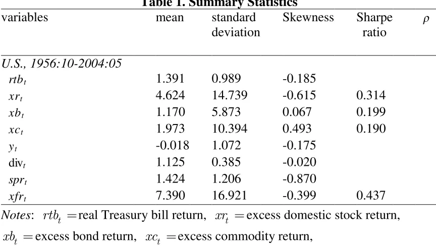
Table 1 reports the mean, variance, and skewness for the bill, bond,

stock and commodity returns and three instruments. The entries for mean and

standard deviations are expressed in percentage. The Sharpe ratios for the bond,

stock and commodity returns are reported in the last column. As expected,

Treasury bill has low return as well as low volatility. The mean excess returns for

stocks, bonds and commodities are 4.62%, 1.17% and 1.98%, respectively, and the

standard deviations of them are 14.74%, 5.87% and 10.39%, respectively. Both

the mean returns and volatility for stock and commodity are higher than for bond.

The Sharpe ratio for stock, bond, and commodity are 0.31, 0.19 and 0.20. That is,

Stock has the highest Sharpe ratio. Although commodity has higher volatility than

bonds, its Sharpe ratio is almost the same as for bonds.

[Insert Table 1 Here]

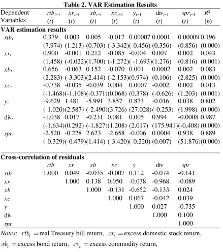
Table 2 reports the estimation results for the VAR system. The top section of the

table reports coefficients estimates and the R2 statistics (with the p-value in the

parentheses) for each equation in the VAR system. The bottom section of the table

reports the cross-correlation matrix of the innovations.

The first row of the table corresponds to the real bill return equation.

The lagged real bill return and commodity return have significant positive and

negative coefficients, respectively. The second row corresponds to the equation for

the excess stock return. None of variables are significant. This confirms that

predicting stock returns is difficult. The third row is the equation for the excess

bond return. The coefficients for the lagged bond return, excess stock return,

commodity return, and yield spread are all significant. The fourth row reports the

results for the equation of commodity. All the coefficients are insignificant, which

implies that there are few correlations between commodities and other risky assets.

This possibly implies commodity could be an important component of portfolio

choice.

The bottom section reports the covariance structure of the innovations in

the VAR system. Unexpected log excess stock returns has very low correlation

with commodity returns, but are highly negatively correlated with shocks to the

log dividend yield, which is consistent with previous empirical evidence

(Campbell, 1991; Stambaugh, 1999). Unexpected log excess bond returns are

negatively correlated with shocks to nominal bill rate, log dividend yield and

Altogether, the correlations between commodity and stock and bond returns

suggest that commodity could play an important role in the process of strategic

asset allocation. We will further explore their implications for optimal

multiple-period portfolio choice.

[Insert Table 2 Here]

3.4. Demands for Domestic Assets

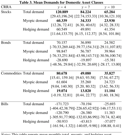
Table 3 reports the mean total, myopic, and intertemporal hedging demands (in

percentage) for domestic bills, stocks, bonds, and commodities for a U.S. investor.

The intertemporal elasticity of substitution is 1. The entries in each column

are mean asset demands when the coefficient of relative risk aversion equal to

4, 7, and 10, respectively. Both the total mean demands and the mean myopic

demands across the four assets sum to 100, while the mean hedging demands sum

to 0. By comparing numbers within each column, we can study how the portfolio

is allocated across the four risky assets and how much is the mean total demand,

myopic demand, and hedging demand for each of the asset classes. By comparing

numbers within each row, we can examine the incremental effects of relative risk

aversion on asset allocation. In addition, the numbers in brackets under each

entry are the 90% confidence intervals for the mean asset demands.

From the table, one can see that the total and myopic demand allocation

is holding a long position on stocks, bonds and commodities, while shorting bills.

commodities. The significant mean total and myopic demand for stocks is

consistent with the theory that there is higher demand for the asset with the largest

Sharpe ratio. In addition, there are positive mean hedging demands for stocks and

commodities. The mean hedging demand for commodities is significant in the

90% confidence interval, though the mean hedging demand for stocks is larger in

magnitude. Both the mean hedging demands for bonds and bills are negative,

which is consistent with the findings in Campbell, Chan, and Viceira (2003) and

Rapach and Wohar (2009). By comparing each row, as we would expect, the mean

total, myopic and hedging demands for all the risky assets decrease as relative risk

aversion increase.

The large mean demands for stocks can be explained by the negative

correlation between innovations to log excess stock returns and the log dividend

yield. As the stock returns have large positive Sharpe ratio, investors usually take

long positions in stocks. An increase in expected stock returns represents an

improvement in the investment opportunity set, while a decrease in expected

stocks returns represents a worsening of the investment set. In addition, the VAR

estimation results suggest that lagged dividend yield has a positive effect on the

expected stock returns. Given the negative correlation between innovations to

excess stock returns and dividend yield, one should expect that a negative shock to

excess stock return next period are accompanied by a positive shock to the

dividend yield next period. In turn, a positive shock to the log dividend yield next

use stocks to hedge against the negative shocks to futures returns.

[Insert Table 3 Here]

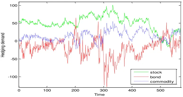
Figure 1 plots the estimated hedging demands for domestic stocks,

bonds, and commodities in order to show more intuitive picture of the

intertemporal hedging demands for each of the three asset class. Overall, the

hedging demand for commodity appears to be the most stable compared with those

for stocks and bonds. And the hedging demand for commodity and stock are well

above the hedging demand for bonds over most of the sample period.

[Insert Figure 1 Here]

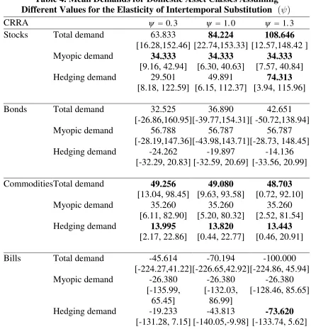
A recent theoretical work by Bhamra and Uppal (2006) suggests that the

elasticity of intertemporal substitution can affect the magnitude, but not the

sign, of the intertemporal hedging demand for the risky asset. Here we compute

the mean demands for stock, bond, and commodity by setting values of

intertemporal substitution equal to 0.3, 1, and 1.5 and the results are presented

in Table 4. The mean total and hedging demands for stocks increase largely as the

intertemporal substitution increases and gradually becomes positively

significant. That is, investors are becoming more willing to make a trade-off

between contemporary and future consumption by taking more long positions on

stocks. Both the mean total and hedging demand for commodities do not change

very much, but are always positively significant as the value of increases. The

provide support for the argument that commodity is an attractive asset class for

multi-period portfolio choice. In addition, our results are also consistent with

Bhamra and Uppal's theoretical results that only affects the magnitude, but not

the sign, of the mean hedging demands for risky assets.

[Insert Table 4 Here]

3.5. What Explains the Demands for Commodities?

What explains the striking and significant mean total and intertemporal hedging

demand for commodities? One explanation might be based on modern portfolio

theory which states the interaction of asset classes with each other provides

diversification. The commodity future return is negatively correlated with bond

return by -0.13 and a very low correlation with the most risky asset, stock return.

These findings suggest commodities have the ability to help diversify stock and

bond portfolios. Furthermore, the low correlation between innovations to stock

and commodity returns is 0.05, which almost approaches zero. Consequently, the

large positive intertemporal hedging demand for stocks does not reduce the

demand for commodities, which may explain why the positive demand for

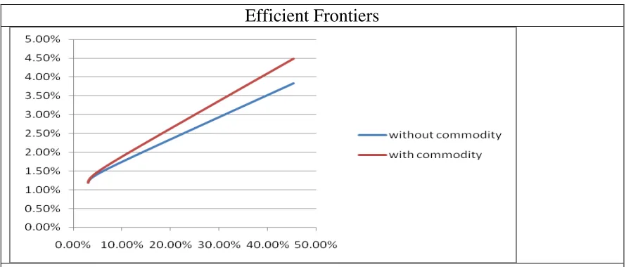
commodities is significant during the long horizons. The portfolios constructed

based on the estimation results provide further evidence to support the explanation.

In figure 3, the portfolio with commodity futures is more efficient, has a higher

ratio of return to risk, than the portfolio without commodity futures.

The second tentative explanation is from the aspect of the return

distributions. It is a well established fact that traditional asset returns, for example,

stock returns, are negatively skewed, and the distribution of commodity returns is

positively skewed. The positive skewness of commodity return together with its

lower volatility relative to stock return, imply that commodity has lower

downward risk compared to equities like stocks. In this study, the skewness for

monthly average excess stock and commodity returns are -0.62 and 0.49, while the

volatilities for them are 14.74% and 10.39%, respectively. If the tail events can

happen simultaneously for the two asset classes, commodity, as an independent

asset class, can provide large diversification benefits to the portfolio allocation.

Another explanation comes from the correlation between commodity

returns and inflation. This is because the ultimate function of portfolios is for

consumption. Thus, investors should consider the real purchasing power of their

returns; that is, the asset classes' ability of hedging against inflation Traditional

asset classes such as stocks and bonds are negatively correlated with inflation and

are not good asset classes for hedging against inflation. However, commodities

represented by commodity futures, may be a better hedge against inflation because

(i) they have a positive correlation with inflation in the long run; (ii) commodity

prices are directly linked to unexpected inflation shocks, which is an important

component of inflation. These together may explain why commodities are a better

asset class of hedging against inflation risk than stocks and bonds.

hedging demand for commodities found in this paper suggest that commodity can

be an attractive asset class to diversify traditional portfolio of stocks and bonds.

4. Controlling for International Stock Markets

To check for the robustness and stableness of the estimated hedging demand for

commodities, we expand the analysis by allowing the investors to access

international equity markets, in addition to domestic stocks, bonds, commodities,

and bills. We use the MSCI World Equity Index ex U.S. as a proxy for foreign

stock market, which makes the calibration not too complicated. In this case,

investors can make a strategic asset allocation across domestic bills, bonds, stocks,

commodities, as well as foreign stocks. We estimate the expanded VAR system

and use the CCV approach to approach the mean total, myopic, and hedging

demands for each of the asset classes. To reserve space, we will not report the

VAR estimation results.

Table 5 reports the mean total, myopic, and intertemporal hedging

demands (in percentage) for domestic bills, stocks, bonds and commodities as well

as foreign stocks for a U.S. investor. The results are computed by setting the

intertemporal elasticity of substitution 1 and the coefficient of relative risk

aversion equal to 4, 7, and 10, respectively. The demands for various asset

classes decrease, as the relative risk aversion increases. The first striking

finding is U.S. investors continue to have relative large mean total and

foreign equity markets, although these demands are no more significant according

to the 90% confidence intervals. However, the mean myopic demand for domestic

stock is essentially low compared to when they can only allocate across domestic

asset classes. The large magnitude in mean total and hedging demands for

domestic stocks is consistent with the well-established theoretical and empirical

finance literature that U.S. investors have home bias (e.g., Cooper and Kaplanis,

1994; Coval and Moskowitz, 1999; Norman and Xu, 2003; Barron and Ni, 2008).

The second striking finding is the significant mean total and myopic demand for

foreign stocks, although the mean total demand is lower relative to the mean total

demand for domestic stocks. This interesting phenomenon can be intuitively

explained based on some summary statistic characteristics of excess domestic and

foreign stock returns. The standard deviations of domestic and foreign stock

returns are almost equal, but the log excess foreign stock returns are almost two

times that for domestic stock. Thus, the foreign stock returns have higher Sharpe

ratio than domestic stock returns. All else equal, investors should have higher

myopic demands for assets with higher Sharpe ratio, which explains why the

myopic demand for domestic stocks is lower for U.S. investors.

The most striking results in Table 5 is the mean intertemporal hedging

demands for commodities. The mean intertemporal hedging as well as the mean

total and myopic demand for commodities are fairly stable compared to when

investors only have access to domestic asset classes. Furthermore, the

after investors can access foreign asset classes. This implies the intertemporal

hedging demands for commodities is stable and confirms commodities should be a

conservative component in strategic asset allocation. To give a direct explanation,

we plot the intertemporal hedging and demands for domestic bonds, stocks, and

commodities, as well as foreign stocks in Figure 2. Overall, the hedging demand

for commodity appears to be the most stable as compared to those for both

domestic and foreign stocks and bonds. Also, the hedging demand for

commodity and stock are well above the hedging demand for bonds and foreign

stocks over most of the sample period.

[Insert Table 5 Here]

[Insert Figure 2 Here]

We also compute the mean demands for stock, bond, and commodity by

setting values of intertemporal substitution equal to 0.3, 1, and 1.5. As shown

in Table 6, investors become willing to make more trade-off between

contemporary and future consumption, i.e., the hedging demands for stock

increase substantially and gradually become positively significant, as the

intertemporal substitution increases from 0.3 to 1.3. Similarly, when investors

can only access domestic asset classes, the mean hedging demand for commodities

changes very little and are always positively significant, as the value of

increases. It confirms again that commodity is effective in portfolio diversification

asset allocation process. In summary, investors in U.S. have significant

intertemporal hedging demands for commodities, in addition to domestic stocks.

This intertemporal hedging demand remains significant in amount, even when

investors have opportunities to invest in other asset classes, for example, foreign

stocks.

In summary, the results above indicate that commodity is one of the

important determinants in the process of strategic asset allocation and multi-period

portfolio choice. There exists a significant and relatively stable intertemporal

hedging demand for commodities, as well as for domestic stocks for U.S.

investors.

[Insert Table 6 Here]

5. The Utility Benefits from Including Commodities

In this section, we differentiate out the importance of the commodity asset class by

comparing the utility of an investor who has access to commodities with the utility

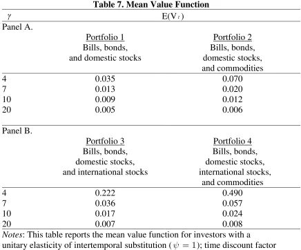
of an investor who does not. Table 7 reports the mean value function when values

of are set to 4, 7, 10, and 20. Panel A compares the mean value function when

two investors can only allocate across domestic asset classes. Panel B compares

the mean value function when two investors can allocate across domestics as well

as international asset classes. The value function is normalized so that a doubling

from one portfolio to another implies that an investor would require twice as much

one.

A comparison of portfolio 1 of panel A, in which commodities are not

included, with portfolio 2 shows that commodities generate large welfare gains for

all investors. Both aggressive and conservative investors gain by allocating some

weights to commodities, which can help hedge against the long positions in

domestic stocks and inflation risk of real interest rates. One can draw the same

conclusion by comparing portfolio 3 and 4 in panel B. In addition, a comparison of

portfolio 1 with portfolio 3 and portfolio 2 with portfolio 4 suggest that the

addition of foreign stocks to an investor's portfolio also creates large gains for all

investors.

[Insert Table 7 Here]

6. Conclusions

Using the Reuters/Jefferies Commodity Research Bureau (CRB) index as a proxy

for commodity, this paper has documented relatively strong and stable

intertemporal hedging demands of U.S. investors for commodity. The result is

robust when other traditional assets, for example, foreign stocks, are included in

the portfolio choice. We also provide evidence that the intertemporal hedging

demand for commodity are relatively stable and permanent in magnitude by

setting the intertemporal substitution and the relative risk aversion to

various values. In addition, the results referring to stock market are consistent with

stock.

A more difficult question is why U.S. investors have a strong

intertemporal hedging demand for the commodity asset class. In this paper, we

have tried to make progress on this question by providing some tentative

interpretations based on modern portfolio theory, return characteristics, as well as

the ability of hedging against inflation. The results presented in this study show,

perhaps interestingly, the significant intertemporal hedging demand for

commodity, because commodity return has low and negative correlations with

traditional asset classes, while having a lower downward risk by having higher

positive skewness. In addition, the surprisingly significant intertemporal hedging

demand for commodity seems to come through its increased ability to hedge

against the unexpected future inflation, compared to traditional assets.

Institution investors have been increasingly interested in commodities

during the past few years. There are currently many intense debates on the role of

commodities in strategic asset allocation. This study provides some new empirical

evidence for advocating commodities as an asset class in portfolio choice. Despite

this, future efforts are needed to build an well-accepted theoretical model on

commodity pricing and to analyze the sources of commodity returns and their role

References

Barron, J. M., and Ni, J., 2008, Endogenous Asymmetric Information and

International Equity Home Bias: The Effects of Portfolio Size and Information

Costs, Journal of International Money and Finance, 27, 4, 617-35.

Bodie, Zvi and Victor Rosansky., 1980, "Diversification Returns And Asset

Contributions", Financial Analysts Journal, (May/June): 26-32.

Balduzzi, P., Lynch, A., 1999, Transaction costs and predictability: some utility

cost calculations, Journal of Financial Economics, 52, 47--78.

Barberis, N.C., 2000, Investing for the long run when returns are predictable,

Journal of Finance, 55, 225--264.

Bhamra, H.S., Uppal, R., 2006, The role of risk aversion and intertemporal

substitution in dynamic consumption-portfolio choice with recursive utility,

Journal of Economic Dynamics and Control, 30 (6), 967--991.

Brennan, M.J., Schwartz, E.S., Lagnado, R., 1997, Strategic asset allocation,

Journal of Economic Dynamics and Control, 21, 1377--1403.

Campbell, J.Y., 1991. A variance decomposition for stock returns. Economic

Journal 101, 157--179.

Campbell, J.Y., Viceira, L.M., 1999, Consumption and portfolio decisions when

expected returns are time varying, Quarterly Journal of Economics, 114,

433--495.

expected returns are time varying: erratum, Unpublished paper, Harvard

University, available on the authors' websites.

Campbell, J.Y., Viceira, L.M., 2001, Who should buy long-term bonds? American

Economic Review, 91, 99--127.

Campbell, J.Y., Viceira, L.M., 2002, Strategic Asset Allocation: Portfolio Choice

for Long-Term Investors, Oxford University Press, Oxford.

Campbell, J.Y., Chan, Y.L., Viceira, L.M., 2003, A multivariate model of strategic

asset allocation, Journal of Financial Economics, 67 (1), 41--81.

Cooper, L., and Kaplanis, E., 1994, Home Bias in Equity Portfolios, Inflation

Hedging, and International Capital Market Equilibrium, Review of Financial

Studies, 7, 1, 45-60.

Coval, J.D., and Moskowitz, T.J., 1999, Home Bias at Home: Local Equity

Preference in Domestic Portfolios, Journal of Finance, 54, 6, 2045-73.

Gorton, Gary, and Geert Rouwenhorst. 2006, Facts and Fantasies about

Commodity Futures. Financial Analysts Journal, 62, 47-68.

Greer, Robert J., 1978, Conservative Commodities a Key Inflation Hedge, Journal

of Portfolio Management, 4(4), 26-29.

Idzorek, M.T., 2008, Strategic Asset Allocation and Commodities, Ibboston

Associates Reports.

Merton, R.C., 1969, Lifetime portfolio selection under uncertainty: the

continuous time case, Review of Economics and Statistics, 51, 3, 247--257.

from Survey Data, Review of Economics and Statistics, 85, 2, 307-12.

Rapach, E.D., and Wohar, E.M., 2009, "International Asset Allocation with

Regime Shifts," Journal of International Money and Finance, 28, 1137--1387.

Lynch, A.W., 2001, Portfolio choice and equity characteristics: characterizing the

hedging demands induced by return predictability, Journal of Financial

Economics, 62, 67--130.

Lynch, A.W., Tan, S., 2010, Multiple Risky Assets, Transaction Costs and Return

Predictability: Allocation Rules and Implications for U.S. Investors, Journal of

Financial and Quantitative Analysis, Forthcoming.

Stambaugh, R.F., 1999. Predictive regressions, Journal of Financial Economics,

Table 1. Summary Statistics

variables mean standard deviation

Skewness Sharpe ratio



U.S., 1956:10-2004:05

rtbt 1.391 0.989 -0.185

xrt 4.624 14.739 -0.615 0.314

xbt 1.170 5.873 0.067 0.199

xct 1.973 10.394 0.493 0.190

yt -0.018 1.072 -0.175

divt 1.125 0.385 -0.020 sprt 1.424 1.206 -0.870

xfrt 7.390 16.921 -0.399 0.437

Notes: rtb_t real Treasury bill return, xr_t excess domestic stock return,

t

xb excess bond return, xc_t excess commodity return,

t

y nominal Treasury bill yield, div_t log dividend yield,

t

Table 2. VAR Estimation Results

Dependent Variables

rtbt1

t

xrt1

t

xbt1

t

xct1

t

yt1

t

divt1

t

sprt1

t R2

p

VAR estimation results

rtbt 0.379 0.003 0.005 -0.017 0.00007 0.0001 0.00009 0.196 (7.974) (1.213) (0.703) (-3.342) (-0.456) (0.356) (0.856) (0.000)

xrt 0.900 -0.001 0.212 -0.085 -0.004 0.007 0.002 0.043 (1.458) (-0.022) (1.700) (-1.272) ( -1.693) (1.276) (0.816) (0.001)

xbt 0.656 -0.063 0.152 -0.070 0.001 0.0002 0.002 0.083 (2.283) (-3.303) (2.414) (-2.153) (0.974) (0.106) (2.825) (0.000)

xct -0.738 -0.035 -0.039 0.004 0.0007 -0.002 0.002 0.013 (-1.468) (-1.108) (-0.371) (0.068) (0.378) (-0.626) (1.203) (0.001)

yt -9.629 1.481 -5.991 3.857 0.873 -0.016 0.038 0.802 (-1.020) (2.587) (-2.490) (3.726) (27.028) (-0.253) (1.998) (0.000)

divt -1.038 0.017 -0.231 0.081 0.005 0.994 -0.0008 0.987

(-1.634) (0.292) (-1.827) (1.208) (2.017) (175.941) (-0.408) (0.000)

sprt -2.520 -0.228 2.623 -2.658 -0.006 0.0004 0.938 0.889

(-0.329) (-0.479) (1.414) (-3.420) (-0.220) (0.007) (51.876) (0.000)

Cross-correlation of residuals

rtb xr xb xc y div spr rtb 1.000 0.049 -0.035 -0.007 0.112 -0.074 -0.141

xr 1.000 0.138 0.050 -0.038 -0.968 -0.089

xb 1.000 -0.131 -0.652 -0.133 0.024

xc 1.000 0.067 -0.042 0.039

y 1.000 0.027 -0.735

div 1.000 0.100

spr 1.000

Notes: rtb_t real Treasury bill return, xr_t excess domestic stock return,

t

xb excess bond return, xc_t excess commodity return,

t

y nominal Treasury bill yield, div_t log dividend yield,

t

Table 3. Mean Demands for Domestic Asset Classes

CRRA   4   7   10

Stocks Total demand 120.889 84.224 65.284

[29.43,196.24] [22.74,153.33] [10.36,121.10] Myopic demand 60.339 34.333 23.930

[12.26, 72.41] [6.30, 40.63] [4.32, 28.33] Hedging demand 60.549 49.891 41.354

[11.64,133.75] [6.15, 112.37] [8.54, 101.86]

Bonds Total demand 70.157 36.890 24.582 [-70.33,269.44] [-39.77,154.31] [-29.11,107.85] Myopic demand 98.847 56.787 39.964

[-76.33,251.84] [-43.98,143.71] [-30.56,100.74] Hedging demand -28.690 -19.897 -15.381

[-48.56, 29.84] [-32.59, 20.69] [-28.17, 13.00]

Commodities Total demand 80.678 49.080 35.827

[15.41, 159.16] [9.63, 93.58] [7.54, 67.27] Myopic demand 61.604 35.260 24.723

[9.04, 140.30] [5.20, 80.32] [3.62, 56.33] Hedging demand 19.074 13.820 11.104

[-0.19, 32.81] [0.44, 22.77] [1.60, 18.36]

Bills Total demand -171.723 -70.194 -25.693 [-404.42,38.79] [-226.65,42.92] [-146.17,53.11] Myopic demand -120.790 -26.380 11.383

[-305.91,77.90] [-132.03,86.99] [-70.74, 82.40] Hedging demand -50.933 -43.813 -37.077

[-161.94,-1.32] [-140.05,-9.98] [-108.88, 0.41]

Notes: This table reports mean monthly total, myopic, and hedging asset demands in percentage for stocks, 10-year government bonds,

commodities and 3-month Treasury bills (cash) for an investor with a unitary elasticity of intertemporal substitution ( 1); time discount

factor equals 0.921/12_{; and coefficient of relative risk aversion ( )}

equal to 4, 7, or 10. Numbers in brackets are Bootstrapped 90% confidence interval. A bold entry indicates significance according

Table 4. Mean Demands for Domestic Asset Classes Assuming

Different Values for the Elasticity of Intertemporal Substitution ( )

CRRA   0. 3   1. 0   1. 3

Stocks Total demand 63.833 84.224 108.646

[16.28,152.46] [22.74,153.33] [12.57,148.42 ] Myopic demand 34.333 34.333 34.333

[9.16, 42.94] [6.30, 40.63] [7.57, 40.84] Hedging demand 29.501 49.891 74.313

[8.18, 122.59] [6.15, 112.37] [3.94, 115.96]

Bonds Total demand 32.525 36.890 42.651 [-26.86,160.95] [-39.77,154.31] [ -50.72,138.94] Myopic demand 56.788 56.787 56.787

[-28.19,147.36] [-43.98,143.71] [-28.73, 148.45] Hedging demand -24.262 -19.897 -14.136

[-32.29, 20.83] [-32.59, 20.69] [-33.56, 20.99]

Commodities Total demand 49.256 49.080 48.703

[13.04, 98.45] [9.63, 93.58] [0.72, 92.10] Myopic demand 35.260 35.260 35.260

[6.11, 82.90] [5.20, 80.32] [2.52, 81.54] Hedging demand 13.995 13.820 13.443

[2.17, 22.86] [0.44, 22.77] [0.46, 20.91]

Bills Total demand -45.614 -70.194 -100.000 [-224.27,41.22] [-226.65,42.92] [-224.86, 45.94] Myopic demand -26.380 -26.380 -26.380

[-135.99, 65.45]

[-132.03, 86.99]

[-128.46, 85.65]

Hedging demand -19.233 -43.813 -73.620

[-131.28, 7.15] [-140.05,-9.98] [-133.74, 5.62]

Notes: This table reports mean monthly total, myopic, and hedging asset demands in percentage for stocks, 10-year government bonds, commodities and 3-month Treasury bills (cash) for an investor with a unitary elasticity of intertemporal of relative risk aversion ( ) equal to 4. Numbers in brackets are

Table 5. Mean Demands for Domestic and International Asset Classes

CRRA   4   7  10

Domestic Total demand 77.01 58.37 46.80 Stocks [-52.30,165.25] [-33.47,134.21] [-22.24,115.66]

Myopic demand 8.60 4.69 3.12 [-45.57, 57.00] [-26.15, 33.60] [-21.50, 19.67] Hedging demand 68.41 53.69 43.68

[-17.88,160.44] [-13.13,134.95] [-6.44, 118.56] Domestic Total demand 127.00 69.27 46.96 Bonds [-17.01,363.00] [-14.35,205.01] [-12.26,142.90]

Myopic demand 141.02 81.08 57.10 [-17.88,337.15] [-9.87, 193.28] [-6.67, 135.73] Hedging demand -14.02 -11.81 -10.14

[-52.75, 65.19] [-37.36, 42.45] [-29.67, 29.65] Commodities Total demand 90.24 55.75 40.99

[34.54, 185.67] [24.52, 113.92] [16.41, 79.62] Myopic demand 63.95 36.62 25.69

[22.05, 162.01] [12.79, 92.76] [8.19, 64.09] Hedging demand 26.29 19.13 15.29

[4.49, 48.52] [4.82, 34.31] [3.97, 25.94] Domestic Total demand -262.15 -122.13 -61.86 Bills [-560.42,-25.35] [-350.23,-5.78] [-202.00,52.93]

Myopic demand -179.07 -59.80 -12.09 [-409.47,-17.48] [-191.68,32.76] [-104.56,52.86] Hedging demand -83.07 -62.33 -49.77

[-204.14, 35.68] [-158.30,-19.19] [-131.86,11.81]

Foreign Total demand 67.90 38.74 27.12

Stocks [-30.03, 115.64] [-16.55, 67.67] [-11.67, 47.47] Myopic demand 65.50 37.41 26.18

[-28.58, 122.47] [-16.24, 69.93] [-11.31, 48.93] Hedging demand 2.39 1.33 0.94

[-9.56, 18.13] [-6.72, 12.32] [-4.20, 10.15]

Table 6. Mean Demands for Domestic and International Asset Classes

Assuming Different Values for Elasticity of Intertemporal Substitution ( )

CRRA   0. 3   1. 0   1. 3

Domestic Total demand 28.03 58.37 121.19

Stocks [-29.82,136.66] [-33.47,134.21] [-26.25,140.56] Myopic demand 4.69 4.69 4.69

[-25.92, 27.65] [-26.15, 33.60] [-28.15, 33.83] Hedging demand 23.35 53.69 116.51

[-8.10, 135.21] [-13.13,134.95] [-20.32,125.89] Domestic Total demand 63.90 69.27 82.51 Bonds [-11.80,202.45] [-14.35,205.01] [-14.98,196.10]

Myopic demand 81.08 81.08 81.08 [-14.93,192.35] [-9.87, 193.28] [0.86, 189.29] Hedging demand -17.18 -11.81 1.44

[-39.66. 39.37] [-37.36, 42.45] [-37.59, 37.94] Commodities Total demand 54.86 55.75 56.00

[16.98, 112.65] [24.52, 113.92] [19.77, 112.32] Myopic demand 36.62 36.62 36.62

[5.92, 91.74] [12.79, 92.76] [8.78, 91.76] Hedging demand 18.24 19.13 19.38

[1.81, 30.46] [4.82, 34.31] [4.89, 32.74] Domestic Total demand -86.69 -122.13 -196.40 Bills [-305.45,30.41] [-350.23,-5.78] [-293.89,24.86]

Myopic demand -59.90 -59.80 -59.80 [-193.18,41.07] [-191.68,32.76] [-167.34,45.80] Hedging demand -26.89 -62.33 -136.61

[-175.51,10.47] [-158.30,-19.19] [-163.24,20.06] Foreign Total demand 39.90 38.74 36.70

Stocks [-16.95, 69.14] [-16.55, 67.67] [-20.97, 73.35] Myopic demand 37.41 37.41 37.41

[-21.66, 65.02] [-16.24, 69.93] [-21.79, 74.26] Hedging demand 2.49 1.33 -0.71

[-6.76, 12.32] [-6.72, 12.32] [-7.20, 12.88]

Notes: This table reports mean monthly total, myopic, and hedging asset demands in percentage for stocks, 10-year government bonds, commodities, 3-month Treasury bills (cash) and foreign stocks for an investor with elasticity

of intertemporal substitution ( 0.3,1,1.3); time discount factor equals 0.92

1/12

Table 7. Mean Value Function

 E(Vt)

Panel A.

Portfolio 1 Portfolio 2 Bills, bonds,

and domestic stocks

Bills, bonds, domestic stocks, and commodities

4 0.035 0.070

7 0.013 0.020

10 0.009 0.012

20 0.005 0.006

Panel B.

Portfolio 3 Portfolio 4 Bills, bonds,

domestic stocks, and international stocks

Bills, bonds, domestic stocks, international stocks,

and commodities

4 0.222 0.490

7 0.036 0.057

10 0.017 0.024

20 0.007 0.008

Notes: This table reports the mean value function for investors with a

0 100 200 300 400 500 -100 -50 0 50 100 Time He dg in g de m an d stock bond commodity

Fig 1. Historical intertemporal hedging demands for domestic stocks, bonds and commodities for U.S. investors.

0 50 100 150 200 250 300 350 400

-100 -50 0 50 100 Time He dg ing d em an d Figure 2. stock bond commodity foreign stock

Fig 2. Historical intertemporal hedging demands for domestic stocks,

Efficient Frontiers