Corruption and the Composition of Public Expenditures: Evidence from OECD Countries

(1)

Munich Personal RePEc Archive

Corruption and the Composition of

Public Expenditures: Evidence from

OECD Countries

Hessami, Zohal

University of Konstanz, Department of Economics

26 September 2010

Online at

https://mpra.ub.uni-muenchen.de/25945/

(2)

Corruption and the Composition of Public

Expenditures: Evidence from OECD Countries

Zohal Hessami

∗

University of Konstanz, [email protected]

Abstract

This paper analyzes how corruption affects the composition of public expenditures. First, a two-stage rent-seeking model with endogenous rent-setting is derived that captures both “political corruption” and “bureaucratic corruption”. The model illustrates how asym-metries between industries in the degree of competition and in the difficulty of concealing bribery may influence the allocation of public spending. The theoretical implications are tested with a panel dataset for 26 OECD countries over the 1996 - 2008 period. The results suggest that the shares of spending on health and environmental protection increase, while the shares of spending on social protection and recreation, culture and religion decline with higher levels of corruption. The significance of these distortions is robust to a variety of specifications such as fixed effects, random effects, seemingly unrelated regressions, the inclusion of additional controls, and the use of alternative corruption indicators.

Keywords: Corruption; rent-seeking; public expenditures; budget composition

JEL codes: D72; D73; H11; H50

∗_{Department of Economics, University of Konstanz, Box 138, 78457 Konstanz, Germany; Phone:}

(3)

1 Introduction

The literature provides robust evidence that corruption is detrimental to the economic devel-opment of a country. More specifically, empirical investigations suggest that an increase in corruption by one standard deviation is associated with an 0.8 to 1.0 percentage point decline in the GDP growth rate (Mauro, 1995; Pellegrini and Gerlagh, 2004). A recent study that benefits from the availability of longer time series of corruption data even suggests a causal link that runs from corruption to economic growth (Swaleheen, forthcoming).1 This causal effect apparently relies on the following transmission channels: investments, trade openness, and political stability (M´eon and Sekkat, 2005; Pellegrini and Gerlagh, 2004).

Firstly, corruption reduces expected returns on investments through an increase in un-certainty and the creation of additional costs. Higher levels of risk associated with returns on investments are due to the difficulty of enforcing bribes (Boycko et al., 1996) and the fact that bribery introduces the risk of being detected. On the other hand, corruption diminishes returns on investments (even when ignoring the risk involved) because it acts as a tax. For instance, when an entrepreneur in a developing country intends to start a business, he may have to bribe a bureaucrat in order to obtain a mandatory business license.

Secondly, policy-makers are likely to create more barriers to trade than is socially opti-mal since trade restrictions can be a substantial source of rents (Krueger, 1974). For instance, a domestic monopolist has an incentive to pay bribes in order to be protected against for-eign competition. Since free trade and international competition increase economic efficiency (Krugman and Obstfeld, 2006), such restrictions cause an impairment of economic growth (Pellegrini and Gerlagh, 2004). Thirdly, the perception that corrupted practices are pervasive in the public sector fuels political discontent and causes instability and violence. Empirical studies (Bardhan, 1997; Jong-A-Pin, 2009; Mo, 2001) point out that such a climate of political instability can be a serious obstacle to economic activity.

A fourth channel, which is relatively neglected in the existing literature, is corruption’s distortionary effect on the allocation of public spending2. Given the growth in public expendi-tures during the past few decades, this transmission channel has most likely gained importance and therefore deserves more attention. The rationale behind a corruption-induced distortion of the public budget is that bribe-maximizing politicians and/or bureaucrats prefer to shift resources to areas with the best opportunities to be bribed. More specifically, they have an incentive to increase the share of public expenditures that is spent on high-technology goods produced in oligopolistic markets (Mauro, 1998), which ensures that bribery is difficult to detect as prices are hardly comparable for innovative products and allows politicians and/or bureaucrats to collect more generous bribes since large profits are at stake.

1

(4)

In line with the fourth transmission channel, Gupta et al. (2001) provide evidence that corruption stimulates military spending, while Mauro (1998) presents cross-sectional evidence that corruption has a negative impact on education expenditures. The neglect of unobserved heterogeneity in Mauro’s cross-country analysis may explain why he does not find a positive association of corruption with defense expenditures in contrast to Gupta et al. (2001), while the time dimension in Gupta et al.’s panel analysis is relatively short (1995 - 2001). Another shortcoming is that both studies mostly rely on data from developing countries, which makes it difficult to draw conclusions with regard to developed countries.

This paper first derives how a distortion in public spending arises in the context of a two-stage rent-seeking model with endogenous rent-setting that captures both “political corruption” and “bureaucratic corruption”. The model illustrates how the number of firms in an industry (representing the degree of competition within an industry) and transaction costs (representing the difficulty of concealing bribery) affect the allocation of public expenditures and the willingness of a politician to make resources available to the rent-seeking contest. To our knowledge, the distortion of public spending due to corruption has so far not been addressed in any existing rent-seeking model in the literature.

The second part of this paper addresses the shortcomings of the aforementioned empirical literature and analyzes the effect of corruption on the composition of public expenditures with panel data for 26 OECD countries that reaches from 1996 to 2008.3 _{Even though the focus}

on a specific group of countries reduces the heterogeneity in the dataset, the cross-country variation in Transparency International’s Corruption Perceptions Index (CPI) is quite large. To be exact, in the data used in this paper the CPI ranges from 0.4 (average for Denmark) to 5.9 (average for Slovak Republic)4. As a third extension to existing studies, the regression analysis includes all ten expenditure categories that are commonly provided instead of a priori assuming that only one or two specific expenditure categories are affected.5

The empirical analysis suggests that an increase in the perceived level of corruption induces a growth in the shares of spending on health and environmental protection, while the shares of expenditures on social protection and recreation, culture and religion decline with increasing corruption. The statistical significance of these effects is robust to a variety of specifications such as fixed effects, random effects, seemingly unrelated regressions, the inclusion of additional controls, and the use of alternative corruption indicators.

The analysis is structured as follows: Section 2 discusses the role that non-competitive market structures and high-technology play with regard to the existence of corruption in the

3

Another reason why we focus on developed countries is that in contrast to the corresponding OECD datasets the GFS data by the IMF on worldwide public expenditures is criticized for its lack of cross-country comparability (Mauro, 1998). Australia, Mexico, Switzerland and Turkey are not included in our sample since data on public expenditures is not available for these four OECD countries.

4

The CPI scale from 0 to 10 has been inverted so that a higher value indicates a higher level of corruption.

5_{Dellavalade (2006) also includes several expenditure categories in her analysis, but focuses on a set of}

(5)

public sector. Section 3 outlines the theoretical background of the analysis in the context of a two-stage rent-seeking model with endogenous rent-setting. Afterwards, section 4 describes the dataset and the empirical strategy, while section 5 reports the results for the baseline estimations and four robustness checks. Finally, section 6 concludes the analysis.

2 Market structure, technology, and public sector corruption

Governments spend the resources that are available to them in various ways. In some cases, governments directly provide services such as education and fire protection. In other cases, governments redistribute income from some members of society to others. In the following, we focus on the kinds of public expenditures that arise when politicians or bureaucrats com-mission firms in the private sector to provide the government with specific goods or services. Examples can be found in the health sector, in the military sector, and with regard to waste management. The objective in this section is to identify what factors make corruption more likely when the government and the private sector interact in such a setting.

In her seminal contribution, Krueger (1974) points out the simple fact that the existence of rents induces rent-seeking behavior.6 Hence, one way to assess where public sector cor-ruption is most likely to occur is to analyze which types of public expenditures promise rents to politicians and/or bureaucrats. Going one step further, it makes sense to analyze which types of public expenditures promise thehighest rents to politicians and/or bureaucrats.

One factor that is strongly related to the size of the rent, which the public official can expect, is the market structure that potential bribers are facing (Rose-Ackerman, 1975). Since the stakes for being awarded a public contract are much higher in a non-competitive than in a competitive setting, a bribe-maximizing politician has an incentive to shift as much of the public resources available to him to types of expenditures which are spent in non-competitive markets (Mauro, 1998). Of course, there is a limit as to how large this distortion will get since the politician wants to keep the probability of detection reasonably low. The impact of the market structure on rent-seeking activities can also be extended to the international sphere given the evidence that corruption prevails in countries where firms have low exposure to foreign competition (Ades and Di Tella, 1999).

(6)

Vishny, 1993). The fact that this is especially true for defense expenditures due to national security reasons is pointed out by Hines (1995) who provides evidence that international trade in military aircraft is particularly prone to corruption.

The bribe that an agent from the private sector is willing to pay in order to succeed in a public invitation to tender increases proportionally with the profits that the briber earns with the involved public project. This line of reasoning implies that corruption induces a shift of public resources to expenditure types that are allocated to large projects (Bardhan, 1997). Since the size of a project increases with the prices of the products bought, this argument is again related to oligopolistic market structures and the fact that high-technology products require large R&D investments. Tanzi and Davoodi’s (1997) finding that public resources are shifted to investments in the building and creation of projects and away from operation and maintenance lends some support to this hypothesis.

To conclude, the above considerations suggest that two main factors affect the likelihood that corruption occurs. First, the number of bribers in an industry that try to induce a shift public expenditures in their favor is negatively correlated with the likelihood that this shift will occur. Second, it is more likely that corruption occurs in fields where it is easy to keep bribery secret, i.e. where products involve high-technology and prices are difficult to ascertain. The following section will integrate these considerations in a two-stage rent-seeking model to illustrate how these two factors affect the composition of public spending. To do so, we divide the private sector into different industries that may be commissioned by the government to provide a good or a service. The government’s purchase of these goods and services in turn gives rise to public expenditures in distinct expenditure categories.

3 A two-stage bribing contest with endogenous rent-setting

3.1 General framework

This section applies the two-stage rent-seeking framework by Katz and Tokatlidu (1996) in the context of public sector corruption. The model is augmented by allowing for an endogenous determination of the size of the rent in line with Appelbaum and Katz (1987). The considerations from section 2 are integrated into this model by means of an asymmetry in the number of firmsnj ≥2 (representing the degree of competition) and an asymmetry in

the effectiveness of rent-seeking effortsβj7 (inversely related to the transaction costs involved

in keeping bribery secret) across two industries j =A, B. The objective is to illustrate how these factors affect the share of the rent that the two industry groups are expected to gain. This in turn sheds light on the question how the allocation of public expenditures is distorted.

7

(7)

The model rests on the assumption that a politician has discretion over the allocation of a budget G > 0 that is exogenously given. The politician can, however, determine what share (1−γ) of the public budget G he wants to make available to the rent-seeking contest and therefore, he is a rent-setter. There are two industries denoted as j =A, B that consist of nj firms and that pay bribesxij to the politician in order to win the rentS = (1−γ)G.

Given that the rent is divisible, each industry wins an expected share of the rentS which represents apublic good at this point. If the politician announces that he will allocate a large share of the public budget G to the rent-seeking contest, he is likely to lose the election and to receive neither any of the bribe income nor his salary in office y. Instead, he earns an alternative compensationV < y.8 _{On the other hand, if the politician announces that a small}

share of G will be allocated to the contest, he is more likely to win the election but he will receive a smaller amount of bribe income when he is in office.

In the second stage, we do not presume that there is an endogenous sharing rule as in Nitzan (1991). Instead, since the recipient of the bribe is now a different person (a bureaucrat) who we assume to be independent from the politician, the second stage constitutes a separate contest and the first-stage bribes by the individual firms are sunk. In this intra-industry bribing contest, the expected share of the rent S represents a private good. Expenditures by each of the firms in the second round are denoted byyij.

In sections 3.2 to 3.4, this model is solved recursively, i.e. the analysis starts out with the second stage. The reason is that the individual firms anticipate in the first stage that they will have to engage in a second-round contest where they have to incur additional expenses in order to win their individual share of the rent.

3.2 Bureaucratic corruption: Bribing contest between firms

In the second stage, the firms in industries AandB compete for their individual share of the rent S by paying bribesyij to a bureaucrat who has complete discretion over the allocation

of his fixed budget. His decision is based entirely on the relative amount of bribes that he receives. More specifically, following Tullock (1980) the share of the rent S that firm iwins is represented by:

pij =

 



yij

yj if max

y₁j, ..., ynjj >0

1

nj else.

(3.1)

8

(8)

Since it has not been derived yet what share ofS is allocated to the two industries, we solve the optimization problem for the case where one of the groups wins the whole rent S in the first stage. Consequently, firm i= 1, ..., nj in industry j=A, B solves:

Max πij =pijS−yij. (3.2)

Assuming a Cournot-Nash equilibrium, an interior solution and symmetric firms within each industry, the size of the bribe that an individual firm pays to the bureaucrat and the sum of bribes paid by an entire industry can be expressed as follows:

yij∗=

nj−1

nj2

S, yj∗ =

nj−1

nj

S. (3.3)

We can infer from these equations that the optimal bribe paid by an individual firm decreases with the number of firms since each firm expects to win a smaller share of the rent. Yet, the sum of bribes paid by an industry increases with the number of firms. If we plug the expression for the optimal bribe paid to the bureaucrat (equation 3.3) into the profit function in equation 3.2, the expected profit of an individual firm is derived as:9

πij∗ =

1

nj2

S. (3.4)

Note that the existence of a second-stage contest causes a waste of resources. If the bureaucrat simply allocates the rent that is intended for a specific industry equally among the individual firms, each firm would have an expected profit of πij∗ = _n1_jS. However, we assume that the

firms mistrust each other and do not rely on the fact that the other firms will abstain from bribing the bureaucrat.

In the case where industry A is characterized by an oligopolistic market structure, whereas firms in industry B operate in a competitive market environment, it holds that

nA < nB, i.e. the number of contestants differs between the two industries. If nA < nB is

fulfilled, equation 3.4 predicts that the expected profit for firms in industryA is higher than for firms in industryB, i.e. πiA∗ > πiB∗.10 If the valuation of firms in industryB for entering

the second round contest is comparatively lower, this is likely to have an influence on the first-stage bidding behavior of this industry. This will be analyzed in the next section.

9

Obviously, the share of the rent that an individual firm obtains (i.e. the value of the project(s) that the firm has been assigned to) does not represent pure profits. However, in order to keep the model tractable we have abstained from introducing an additional parameter that captures the profit margin.

10_{Note that the difference in expected profits between the two industries grows disproportionately with the}

(9)

3.3 Political corruption: Bribing contest between industries

In the first stage of the contest, the politician decides what share of the rent S to allocate to each of the two industries. His decision depends on the relative size of the bribes that he receives from the two industries. When industry j collectively expends xj, the politician

receives βjxj with 0< βj ≤1.

The parameter βj is introduced in order to reflect the fact that the transaction costs

involved in keeping the bribe payment secret may differ between the two industries. The larger βj is, the lower are the transaction costs. In conclusion, the share of the rent S that

the firms in industry j=A, B obtain is represented by:

Pj =

 



βjxj

βjxj+βjxj if max{xj, xj}>0

1

2 else.

(3.5)

Even though the politician allocates S according to the relative size of the aggregate bribes in each industry, each firm decides individually on the size of the bribe xij that is paid to

the politician. The profit that an individual firm can expect when entering the second round of the contest is represented by πij∗ (see section 3.2). Based on these considerations, each of

the nj symmetric firms in industryj =A, B solves the following maximization problem:

Max Πij =Pjπij∗−xij. (3.6)

The first-order condition for this optimization problem can be written as follows:

βjβj

X

i=1

nj

xi jS− βj

X

i=1

nj

xij +βj

X

i=1

nj

xi j

!2

nj2= 0. (3.7)

If we use the fact that the firms are symmetric within the two industries, we obtain:

njβjβjxi jS−(njβjxij +njβjxi j)2nj2 = 0. (3.8)

Further manipulation of equation 3.8 yields the following expression that describes the rela-tionship between the total expenditures of the two industries in equilibrium:

xj∗ =xj∗

nj2

(10)

Finally, we combine equations 3.8 and 3.9 to obtain the equilibrium expenditures by industry

j. As the following expression shows, this amount depends on the number of firms in each industry, the transaction costs in making a bribe payment, and the size of the total rent:

xj∗ =

βjβj

nj2(βjnj

2

nj2 +βj)

2S. (3.10)

On the basis of equation 3.10, it is straightforward to derive the politician’s total bribe income (βjxj∗+βjxj∗), which we denote asR1:

R₁ =





βj

nj2(βjnj

2

nj2 +βj)

2 +

βj

nj2(βjnj

2

n2

j +

βj)2



βjβjS. (3.11)

Equation 3.11 suggests that the larger the rent S is, the more bribe income is collected by the politician. However, the influence of the number of firms and the size of transaction costs is less obvious at this point (see section 3.4 for such comparative statics analyses).

3.4 Endogenous rent-setting

Following Appelbaum and Katz (1987), the politician is at the same time a rent-seeker and a rent-setter. Therefore, the size of the rent is determined endogenously. More specifically, the politician is torn between two objectives. He wants to be elected and earn a high salary

y, but on the other hand he also wants to collect a high bribe incomeR1.

Both of these objectives depend on what share (1−γ) (with 0 ≤ γ ≤ 1) of the total budget G he makes available to the rent-seeking contest (S = (1−γ)G). When γ is large, the rent S is small and following equation 3.11 the politician’s bribe income will be low. On the other hand, a large γ increases the probability gthat the politician wins the election and receives a high salary. In summary, the politician faces the following objective function:

Max E[U] =g(γ)(y+R₁) + (1−g(γ))V. (3.12)

In order to allow for an explicit solution for equation 3.12, we assume g(γ) = γ. The max-imization of equation 3.12 yields the following expression for the equilibrium share of the budget Gthat is not allocated to the rent-seeking contest:

γ∗ = 1 2 +

y−V

2κG with κ=





βj

nj2(βjnj

2

nj2 +βj)

2 +

βj

nj2(βjnj

2

n2

j

+βj)2



(11)

Equation 3.13 shows that the politician makes less than half of the total budgetGavailable as a rent for the bribing contest under the assumption that y > V holds. In addition, since

γ∗ _≤ _{1 has to be fulfilled, we know that} _G _≥ y−V

κ . Hence, the total budget has to be large

enough or conversely the salary gain from being elected into office should be moderate. Based on equation 3.13, one can easily derive the following relationships:

∂γ∗ ∂y >0,

∂γ∗

∂V <0, and ∂γ∗

∂G <0. (3.14)

Equation 3.14 suggests that the politician’s motivation to abstain from making public re-sources available for the rent-seeking contest depends positively on the size of his salary when in office y and negatively on his alternative wage V. This corresponds with the existing evidence in the empirical (Van Rijckeghem and Weder, 2001) and experimental literature (Schulze and Frank, 2003) for a negative relationship between the wage level in the public sector (compared to the wage level in the private sector) and corruptibility.

Finally, the larger the overall budget G is, the higher is the potential bribe income of the politician and the more public resources will he make available as a prize for the bribing contest. This aspect is particularly noteworthy when considering the growth in public sector size over the past few decades because it points out that distortions in the allocation of public budgets have become more significant over time.

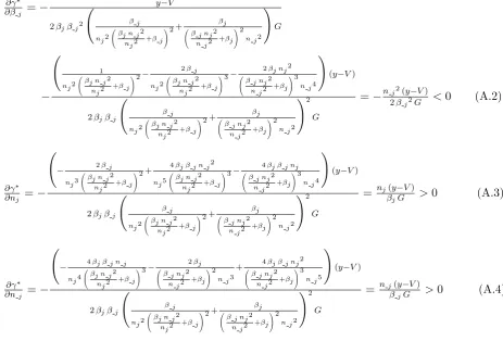
In addition to the relationships summarized in equation 3.14, one can derive how γ∗

is influenced by the number of firms and the size of the transaction costs in each industry (complete derivations are provided in appendix A):

∂γ∗ ∂βj

<0, ∂γ

∗ ∂βj

<0, ∂γ

∗ ∂nj

>0 and ∂γ

∗ ∂nj

>0. (3.15)

It follows from equation 3.15 that higher transaction costs (1−βj or 1 −βj) associated

(12)

4 Data and model specification

4.1 Data description

The dependent variable in the estimations is one of ten expenditure types as a share of total public expenditures taken from the OECD National Accounts database (see table 6 in the appendix for a definition of these expenditure types). Even though theabsolute amount of public resources spent on purposes such as social protection is unlikely to be affected by corruption in the way described in sections 2 and 3, we include these expenditure types in the regression analysis since it is still possible that the relative shares are affected.

[image:12.595.178.422.434.611.2]

Corruption is the main explanatory variable in the empirical analysis and is measured by the Corruption Perceptions Index (CPI) from Transparency International. This data is of a subjective nature since the CPI relies on surveys among international business people, risk analysts, local residents and expatriates. Figure 1 illustrates averages for the CPI from 1996 to 2008 for each of the 26 OECD countries. Obviously, corruption is lowest in Scandinavian countries, whereas the most corrupt countries are mainly located in Eastern Europe and the Mediterranean region. The CPI averages exhibit a high cross-country variation with values ranging from less than 1 until up to 6 on a scale from 0 to 10.

Figure 1: Corruption averages per country, 1996 - 2008

Source: Transparency International

(13)

is not a trivial finding given that one might expect foreign experts to have different perceptions of the incidence of corruption in a country than residents and local businessmen. Third, Kaufmann et al. (2004) investigate the potential for biases in perceptions more specifically and report that they do not find any significant ideological biases in corruption ratings. Finally, it has been argued that the CPI allows for year-to-year comparisons even if the sources used are not the same in each year. This is due to the fact that the effect of changes in the sources on the CPI estimate is rather small (Lambsdorff, 2004b).

In order to accommodate the fact that demographic factors have a strong influence on the composition of the public budget, we include the age-dependency ratio based on the OECD Annual Labour Force Statistics (ALFS) in all the estimations. In addition, the regressions control for population density since the provision of public goods should be cheaper in more densely populated areas due to economies of scale. Moreover, we take into account the share of the urban population in all estimations since preferences for the provision of public goods and services are likely to differ between urban and rural areas. The data for both population-related variables is taken from the World Bank’s World Development Indicators.

In addition, we include the growth rate of real GDP as one of two economic variables from the OECD databases in the regressions due to Wagner’s Law. According to this rule, the public sector grows as a society becomes wealthier based on two arguments. Firstly, as states grow wealthier they also grow more complex, increasing the need for public regulatory action. Secondly and more importantly, certain publicly provided goods such as education are luxury goods only provided when society reaches a certain level of wealth. In addition, we include the unemployment rate given that the relative importance of social protection expenditures in the public budget is likely to increase with high levels of unemployment.

The estimations also take into account several fiscal policy variables. First, we control for government size (total expenditures divided by GDP). Second, the estimations include gross financial liabilities of the general government as a share of GDP. A government that faces high levels of debt is likely to temporarily cut expenditures in certain areas. Third, we include the interest rate on government bonds as a catch-all measure for the fiscal situation in a certain country. This has the advantage that we can capture government stability and political risks. All three variables are taken from the OECD Annual National Accounts.

(14)

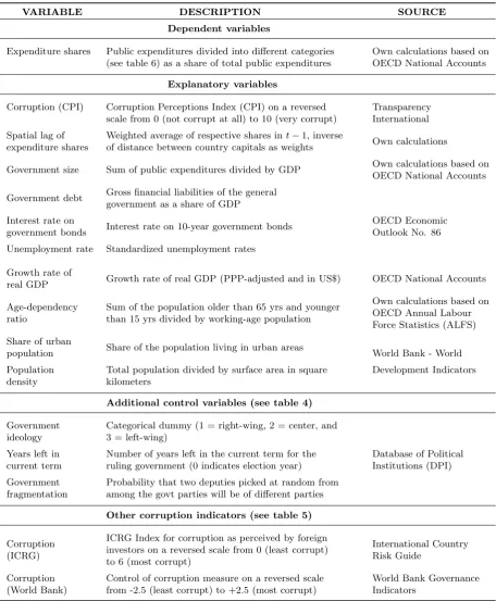
government coalition and their relative sizes are likely to affect how the budget is allocated (for a more detailed definition of the political variables see table 7).11

Moreover, we use two alternative measures for corruption as a robustness check. The first measure belongs to the World Bank Governance Indicators (Kaufmann et al, 2004). While this measure is an aggregate indicator like the CPI, one of the main advantages is that it uses more sources than the CPI. As a result, the World Bank corruption measure captures corruption in the public as well as the private sector (some sources provide data on corruption at the household level) as perceived by experts and opinion polls, while the CPI measures public sector corruption as perceived by experts only. We do not use the World Bank’s corruption measure in the baseline estimations because it has only been published bi-annually prior to 2002. The second corruption measure that we use as a robustness check is provided by the private risk-rating agency Political Risk Services, Inc. that publishes the International Country Risk Guide (ICRG). The advantage of the ICRG corruption measure is that it is not a composite indicator and therefore year-to-year comparisons are more reliable.12

4.2 Empirical strategy

In addition to being affected by the extent of corruption and the control variables outlined in the previous section, the budget composition in a country may also be directly influenced by the budget composition in other countries. In line with Devereux et al. (2008), the policy reaction function in this particular case can be expressed as follows:

Expshare_it =Ri(Expshare−i,t−1, Zit). (4.1)

In equation 4.1 the term Expshareit represents the respective expenditure category, while

Expshare−i,t−1captures the vector of expenditure shares in all other countries in the previous

period. Finally, Zit stands for all remaining factors that influence the budget composition

including the extent of corruption.

Since equation 4.1 cannot be estimated given the available degress of freedom, Devereux et al. (2008) recommend to replace the vector Expshare−i,t−1 by weighted averages. As

weightsωij, we choose the inverse of the spatial distance between the capitals of the countries

in our sample, since countries are more likely to respond to fiscal policy changes in countries that are closeby rather than geographically distant. Summarizing, we estimate the following equation for each of the ten expenditure categories:

Expshare_it=αi+βCorruptionit−1+γ X

j6=i

ωijExpsharejt−1+δXit+νt+ǫit, (4.2)

11

For evidence on the relationship between fragmentation and fiscal policy see Ricciuti (2004) and Volkerink and de Haan (2001).

12

(15)

where the subscripts refer to a country i = 1,2, ...,26 and the respective time period t = 1996,1997, ...,2008 . ǫit represents the normally distributed error term.

Corruptionit−1 measures the lag of perceived corruption in a country according to the

CPI index from Transparency International. We have chosen to lag this variable in order to take into account potential endogeneity problems and to accomodate the fact that corruption is unlikely to have an immediate effect on budgetary measures. Xit is a vector that includes

the age-dependency ratio, the share of the urban population, the growth rate of real GDP, and the unemployment rate. All regressions include time dummies in order to control for common exogenous shocks νt and an intercept αi in order to deal with unobserved hetereogeneity.

Moreover, hypothesis tests are based on standard errors that are robust to heteroscedasticity. It is finally important to note that the spatially weighted expenditure shares also enter the regressions with a lag. This is preferable from a theoretical perspective since fiscal policy responses to changes in neighboring countries are likely to take time. From an econometric perspective, it is additionally advantageous to lag this variable since the potential endogeneity problem with regard to these averages is solved without relying on the use of instrumental variables (Devereux et al., 2008).

The estimation results for the two-way fixed effects models are presented in section 5.1. The baseline estimations are followed by four robustness checks (section 5.2) that involve random effects, seemingly unrelated regressions, the inclusion of additional controls, and the use of alternative corruption measures.

5 Estimation results

5.1 Baseline regressions

(16)

One example of anecdocatal evidence is the Cologne incinerator project in Germany, where allegedly US $13 million were paid in bribes during the construction of a US$ 500 million waste incineration plant (Transparency International, 2005). A second example is the Naples waste management crisis that peaked in the summer of 2008 (Smoltczyk, 2008). In this particular case, municipalities awarded expensive waste disposal contracts to shady consortiums controlled by the local Mafia. After fourteen years and a total cost of $ 2 billion none of the three waste incinerators were operational and the garbage piled up on the streets of Naples. An alternative explanation for the observed positive correlation could be that corruption represents a major obstacle to environmental protection as it helps companies to circumvent laws and regulations (Fredriksson and Svensson, 2003; Pellegrini and Gerlagh, 2006; Woods, 2008). In the long run, this should lead to a deterioration in environmental quality that creates a need for higher expenditures on environmental protection.

Since public spending on social protection merely represents redistributive transfers be-tween different population groups that are unlikely to be influenced by bribe-paying firms, the relative importance of this expenditure category decreases with corruption. This does not necessarily imply that expenditures in this area are cut, but only that the relative share significantly shrinks. In addition, public spending on recreation, culture and religion de-creases as well relative to other expenditure categories, which is in line with the theoretical considerations in sections 2 and 3 as they also provide very few opportunities for bribery.

The magnitudes of the coefficients for corruption in table 1 can be interpreted as follows: An increase in perceived corruption leads ceteris paribus to an increase in expenditures on health and environmental protection by 0.4 and 0.05 percentage points, respectively. In addition, this change leads to a decrease in expenditures on social protection and recreation, culture and religion by 0.3 and 0.04 percentage points.13 _{With regard to the control variables,}

it can be stated that the ten expenditure categories are in most cases significantly affected by demographic factors, fiscal policy shocks in neighboring countries, the economic situation in a particular country and other fiscal policy variables (government size, government debt, and interest rate on government bonds). In addition, the country and time fixed effects are jointly significant at the 1% level, respectively.

To conclude, by focusing on developed countries and using a longer time series in addition to panel-specific estimation techniques we observe corruption-induced changes in the relative importance of expenditure categories that are quite different from those observed by Mauro (1998) and Gupta et al. (2001). However, they are in line with our theoretical predictions in sections 2 and 3. Apart from the fact that we use alternative estimation techniques and other data sources, there is an additional reason why we obtain different results.

13

(17)

[image:17.595.100.756.139.444.2]

Table 1: Estimation results with fixed effects, 1996 - 2008

Model 1a Model 2a Model 3a Model 4a Model 5a Model 6a Model 7a Model 8a Model 9a Model 10a

Social Health Education Defense General Public Economic Housing & Environ- Recreation, protection public order & affairs community mental culture and

services safety amenities protection religion Corruption (t−1) -0.281** 0.428*** 0.065 -0.110 -0.163 0.029 0.005 0.049 0.054* -0.038*

(-2.494) (5.737) (1.221) (-1.488) (-1.355) (0.888) (0.021) (0.892) (1.886) (-1.756) Spatially weighted -0.097 0.466*** -0.573*** -0.241*** -0.095 -0.092 -0.098 -0.298*** -0.242* 0.224** exp. shares (t−1) (-0.967) (3.195) (-5.709) (-4.311) (-0.463) (-1.036) (-0.385) (-3.023) (-1.762) (2.465) Government size -0.116*** -0.085*** -0.061*** 0.009 0.062 -0.023*** 0.117** 0.046*** 0.019** 0.013

(-5.409) (-3.221) (-4.314) (0.677) (1.347) (-2.910) (2.035) (4.289) (2.120) (1.291) Government debt 0.029*** 0.009** -0.012*** -0.006** 0.029** -0.001 -0.038*** -0.004 -0.008*** -0.005***

(6.889) (2.488) (-9.607) (-2.351) (2.188) (-0.763) (-3.287) (-1.531) (-8.805) (-3.528) Interest rate on -0.428*** -0.218*** 0.080* 0.081* 0.275*** 0.045** 0.130 0.062 -0.058*** 0.036 government bonds (-3.504) (-3.059) (1.799) (1.914) (4.837) (2.532) (0.914) (1.544) (-4.259) (1.482) Growth rate of -0.080** 0.070* 0.028 0.033* -0.012 0.032** -0.082 -0.012 -0.003 0.020* real GDP (-2.239) (1.763) (1.550) (1.678) (-0.214) (2.035) (-1.250) (-0.455) (-0.369) (1.921) Unemployment 0.421*** -0.238*** -0.036* 0.012 0.043 -0.038* -0.170*** 0.016 -0.046*** 0.025*** rate (6.463) (-6.964) (-1.855) (0.574) (0.839) (-1.878) (-2.621) (0.752) (-4.383) (2.594) Age-dependency 34.478*** -2.305 -5.020*** 2.453 -24.335*** 1.041 1.478 -2.327*** -3.879*** -0.735 ratio (8.513) (-0.806) (-4.039) (1.261) (-5.389) (0.862) (0.262) (-2.727) (-6.632) (-0.636) Share of urban 0.130*** 0.279*** -0.040 0.007 0.088 0.031** -0.473*** -0.002 0.003 -0.038*** population (3.440) (4.683) (-0.886) (0.242) (1.309) (2.254) (-7.827) (-0.101) (0.174) (-3.154) Population -0.139*** 0.056*** 0.006 -0.074*** 0.083*** 0.005 0.037** -0.003 -0.003 0.029*** density (-11.820) (2.861) (1.269) (-11.713) (3.581) (1.289) (2.437) (-0.281) (-0.830) (3.796) R2

0.512 0.626 0.316 0.301 0.566 0.248 0.263 0.126 0.350 0.317

Observations 273 273 273 273 273 273 273 273 273 273

1 _{Hypothesis tests are based on panel-corrected standard errors that are robust to heteroscedasticity} 2 _{t-statistics in parentheses}

(18)

In developing countries, a relative increase in the defense budget is more likely to be detected by the press and the general public. The same is true when level of education spending changes. In addition, since developing countries are usually characterized by a democratic political system, politicians are more likely to be punished in upcoming elections if they distort the composition of public expenditures in sensitive areas such as education and defense. Therefore, the exact nature of the distortions that occur due to corruption are likely to depend on the development status of a country.

5.2 Sensitivity analysis

Two-way fixed effects estimations only take into account the within-variation of the data. Since existing investigations mostly rely on cross-sectional estimations and since the Hausman test does not clearly indicate whether we should use random or fixed effects, we are now investigating to what extent the results change with random effects.14 The key difference is that in fixed effects estimations one assumes that the time-invariant characteristics of a country are correlated with the explanatory variables, while in random effects estimations they are not correlated. In table 2, we collect these additional estimation results.

The most interesting insight gained from table 2 is that with random effects the rela-tionship between corruption and the composition of public expenditures is almost the same as with country fixed effects. As in table 1 expenditures on health and environmental pro-tection increase significantly, while expenditures on recreation, culture and religion decline significantly. However, the coefficient for corruption in the model for social protection expen-ditures is still negative but not significant with a t-statistic of -1.06. The magnitudes of the coefficients also only change slightly and are quite robust compared to the results in table 1. In addition, the coefficients for lagged corruption are in two cases more significant than in table 1 (10% level). For environmental protection, the coefficient is now even significant at the 5% level, while for recreation, culture and religion it is significant at the 1% level.

The second robustness check estimates the ten models in table 1 as a system rather than estimating each equation separately. Since the ten expenditure categories sum up to a total of 100%, the regressions for each of the categories are by definition not independent from each other. In fact, when one of the shares decreases, we have the additional information that at least one of the other shares must have increased. Zellner’s (1962) Seemingly Unrelated Regressions (SUR) model makes use of this information. This particular estimation procedure allows for an improvement in efficiency compared to estimating the ten models separately with OLS. The results for this robustness check are summarized in table 3.

14

(19)

[image:19.595.100.755.144.448.2]

Table 2: Robustness check I: Estimation results with random effects, 1996 - 2008

Model 1b Model 2b Model 3b Model 4b Model 5b Model 6b Model 7b Model 8b Model 9b Model 10b

services safety amenities protection religion Corruption (t−1) -0.182 0.296*** -0.026 0.001 -0.077 0.058 0.206 0.066 0.063** -0.090***

(-1.064) (2.713) (-0.404) (0.018) (-0.508) (1.500) (1.258) (1.349) (2.254) (-2.969) Spatially weighted 0.213 0.429** -0.328* -0.171 0.028 -0.022 -0.194 -0.337* -0.208 0.142 exp. shares (t−1) (1.452) (2.522) (-1.936) (-1.084) (0.110) (-0.185) (-1.251) (-1.692) (-1.119) (0.834) Government size -0.130*** -0.089** -0.063*** -0.053* 0.107** -0.029*** -0.019 0.021 0.010 0.031***

(-2.690) (-2.366) (-2.585) (-1.949) (2.369) (-2.661) (-0.455) (1.314) (1.020) (2.799) Government debt 0.029*** 0.010 -0.011*** -0.001 0.066*** -0.001 -0.029*** -0.005** -0.007*** -0.007***

(3.808) (1.506) (-2.984) (-0.395) (6.526) (-0.523) (-4.070) (-2.432) (-4.547) (-4.651) Interest rate on -0.361*** -0.374*** 0.083 0.116 0.294 0.039 0.218 0.048 -0.059** 0.041 govt bonds (-2.931) (-3.874) (1.436) (1.109) (1.144) (1.001) (1.402) (1.069) (-2.414) (1.195) Growth rate of -0.097* 0.014 0.034 0.028 -0.040 0.032* -0.021 -0.014 -0.005 0.030** real GDP (-1.673) (0.253) (1.134) (0.703) (-0.298) (1.933) (-0.325) (-0.949) (-0.496) (2.160) Unemployment 0.431*** -0.228*** -0.048 -0.008 -0.052 -0.030 -0.218*** 0.021 -0.049*** 0.028* rate (5.317) (-3.878) (-1.336) (-0.234) (-0.599) (-1.408) (-2.603) (1.053) (-4.021) (1.762) Age-dependency 36.122*** 2.465 -6.153** 0.695 -31.609*** 0.601 -13.135** -2.922 -4.117*** -0.862 ratio (5.103) (0.462) (-2.005) (0.232) (-3.845) (0.430) (-2.311) (-1.361) (-3.716) (-0.452) Share of urban -0.031 0.078*** 0.079** -0.003 0.016 0.004 -0.082** -0.005 0.004 0.026* population (-0.302) (2.826) (2.458) (-0.094) (0.488) (0.214) (-2.239) (-0.400) (0.380) (1.669) Population -0.013* -0.012*** -0.007*** -0.001 -0.000 0.001 0.009** 0.002* 0.002* 0.000 density (-1.657) (-4.357) (-2.583) (-0.370) (-0.056) (0.835) (2.294) (1.825) (1.950) (0.187) R2

0.197 0.507 0.379 0.190 0.652 0.318 0.490 0.189 0.326 0.309

Observations 273 273 273 273 273 273 273 273 273 273

1 _{Hypothesis tests are based on standard errors that are robust to heteroscedasticity} 2 _{t-statistics in parentheses}

(20)

[image:20.595.99.757.143.447.2]

Table 3: Robustness check II: Estimation results with fixed effects (Seemingly unrelated regressions), 1996 - 2008

Model 1c Model 2c Model 3c Model 4c Model 5c Model 6c Model 7c Model 8c Model 9c Model 10c

services safety amenities protection religion Corruption (t−1) -0.282* 0.396*** 0.057 -0.107 -0.172 0.031 0.005 0.058 0.054* -0.038

(-1.787) (3.081) (0.813) (-1.464) (-0.883) (0.831) (0.030) (1.047) (1.892) (-1.121) Spatially weighted -0.038 0.013 -0.183* -0.081 -0.009 -0.008 -0.057 -0.072 -0.115 0.091 expend. shares (t−1) (-0.569) (0.181) (-1.804) (-0.792) (-0.118) (-0.058) (-0.792) (-0.675) (-0.875) (0.810) Government size -0.117** -0.082** -0.051** 0.009 0.064 -0.023** 0.117** 0.045*** 0.018** 0.015

(-2.574) (-2.213) (-2.501) (0.430) (1.143) (-2.179) (2.367) (2.868) (2.221) (1.522) Government debt 0.029*** 0.013** -0.011*** -0.006 0.030*** -0.001 -0.038*** -0.004 -0.008*** -0.005***

(3.565) (1.992) (-3.163) (-1.521) (2.987) (-0.344) (-4.369) (-1.343) (-5.380) (-2.700) Interest rate on -0.426*** -0.231*** 0.082* 0.091* 0.270** 0.046* 0.128 0.060* -0.060*** 0.037* government bonds (-4.095) (-2.730) (1.764) (1.875) (2.106) (1.878) (1.137) (1.659) (-3.159) (1.675) Growth rate of -0.081 0.063 0.036 0.035 -0.016 0.033*** -0.082 -0.011 -0.003 0.020* real GDP (-1.594) (1.539) (1.587) (1.507) (-0.249) (2.707) (-1.494) (-0.605) (-0.289) (1.827) Unemployment rate 0.425*** -0.233*** -0.030 0.009 0.040 -0.039*** -0.171*** 0.017 -0.046*** 0.025*

(7.146) (-4.826) (-1.135) (0.341) (0.553) (-2.751) (-2.651) (0.806) (-4.307) (1.941) Age-dependency ratio 34.427*** -3.302 -5.290** 2.723 -25.319*** 1.049 1.743 -1.996 -3.745*** -0.736

(6.030) (-0.711) (-2.085) (1.030) (-3.571) (0.778) (0.281) (-1.003) (-3.592) (-0.602) Share of urban 0.133 0.288*** -0.034 0.008 0.098 0.030 -0.477*** -0.009 0.001 -0.036* population (1.371) (3.656) (-0.790) (0.181) (0.813) (1.315) (-4.526) (-0.276) (0.071) (-1.737) Population density -0.138*** 0.060*** 0.004 -0.073*** 0.083*** 0.005 0.036 -0.003 -0.003 0.029***

(-5.612) (3.029) (0.403) (-6.448) (2.736) (0.808) (1.367) (-0.383) (-0.720) (5.523) R2

0.512 0.613 0.305 0.299 0.566 0.247 0.263 0.121 0.349 0.316

Observations 273 273 273 273 273 273 273 273 273 273

3 _{Stars indicate significance at 10% (*), 5% (**) and 1% (***)} 4

(21)

While the coefficients for corruption in the previous period are significant and have the same sign with regard to the models for social protection, health and environmental protection, corruption has an insignificant effect on expenditures on recreation, culture and religion. However, the t-statistic is still negative witht= −1.12. Hence, as with the first robustness check we find confirmation of the significant results in table 1 in three out of four cases.

The third robustness check re-estimates the models in table 1 while adding three political control variables. It should be noted that for the time period considered, there is no data available for government ideology in the DPI with regard to the Slovak Republic. Therefore, the number of countries included in the regressions drops to 25, while the total number of observations drops from 273 to 268. The results for this robustness check are summarized in table 4 and provide additional support for the findings in table 1. The coefficients for lagged corruption have the same sign and significance as in table 1, except that in the model for social protection expenditures (model 1d) the coefficient is now even significant at the 1% level. Furthermore, the coefficients for government ideology and government fragmentation are in most cases significant, while we find only weak evidence for political cycles in the allocation of the public budget. More specifically, the estimation results suggest that left-wing parties spend a higher share of the public budget on social protection and health, while right-wing parties are likely to spend more on public order and safety. In addition, government fragmentation has a significant influence on seven out of ten expenditure shares.

As a final robustness check, we have re-estimated the models for expenditures on social protection, health, general public services, environmental protection and recreation, culture and religion with two alternative corruption indicators. The analysis is limited to these five models since the lagged corruption coefficient has not been significant in any of the other five models in tables 1 to 4. Columns 2 to 6 in table 5 report the results for the estimations that use the ICRG Corruption Index, while columns 7 to 11 refer to the estimations that use the World Bank Corruption Indicator. Since the World Bank measure is only available bi-annually prior to 2002, we have interpolated the values for 1997, 1999, and 2001. Moreover, the estimations in columns 2 to 6 only cover the time period until 2006.

(22)

[image:22.595.103.752.109.484.2]

Table 4: Robustness check III: Estimation results with fixed effects (political control variables), 1996 - 2008

Model 1d Model 2d Model 3d Model 4d Model 5d Model 6d Model 7d Model 8d Model 9d Model 10d

services safety amenities protection religion Corruption (t−1) -0.321*** 0.476*** 0.070 -0.105 -0.185* 0.041 -0.011 0.060 0.054* -0.039* (-2.832) (5.695) (1.496) (-1.480) (-1.883) (1.348) (-0.049) (1.135) (1.906) (-1.718) Spatially weighted -0.064 0.523*** -0.497*** -0.184** 0.019 -0.066 -0.026 -0.210* -0.196 0.256** exp. shares (t−1) (-1.220) (3.570) (-5.753) (-2.157) (0.103) (-0.713) (-0.118) (-1.865) (-1.342) (2.179) Government size -0.129*** -0.070*** -0.056*** 0.009 0.071* -0.018*** 0.109** 0.038*** 0.018** 0.010

(-7.031) (-3.089) (-3.780) (0.596) (1.654) (-3.036) (2.067) (3.555) (2.031) (0.891) Government debt 0.028*** 0.004 -0.013*** -0.006** 0.033*** -0.001 -0.036*** -0.004 -0.008*** -0.004***

(8.325) (1.463) (-12.649) (-2.095) (2.605) (-0.934) (-2.958) (-1.384) (-8.715) (-3.186) Interest rate on -0.475*** -0.264*** 0.065 0.087* 0.336*** 0.047*** 0.149 0.077** -0.057*** 0.045* govt bonds (-3.984) (-3.983) (1.405) (1.930) (5.449) (2.990) (1.090) (2.154) (-3.878) (1.882) Growth rate of -0.065** 0.029 0.019 0.026 0.006 0.025* -0.057 -0.011 -0.004 0.024** real GDP (-2.008) (0.831) (1.042) (1.486) (0.103) (1.836) (-0.966) (-0.444) (-0.408) (2.276) Unemployment 0.390*** -0.185*** -0.023* 0.022 0.019 -0.024** -0.198*** 0.015 -0.046*** 0.020 rate (8.912) (-6.258) (-1.849) (1.446) (0.500) (-2.433) (-2.787) (0.783) (-4.496) (1.607) Age-dependency 33.913*** 2.866 -3.794*** 2.882* -28.459*** 1.698*** -1.100 -2.705*** -3.826*** -1.352 ratio (11.017) (1.054) (-3.450) (1.856) (-7.283) (2.610) (-0.171) (-3.382) (-7.197) (-1.139) Share of urban 0.200*** 0.272*** -0.049 -0.015 0.099 0.005 -0.511*** 0.005 0.007 -0.035*** population (4.321) (5.233) (-1.300) (-0.798) (1.638) (0.421) (-6.780) (0.325) (0.403) (-2.697) Population -0.134*** 0.064*** 0.012** -0.071*** 0.069*** 0.008** 0.033** -0.009 -0.004 0.026*** density (-10.672) (3.064) (2.093) (-10.336) (3.139) (2.177) (2.091) (-0.961) (-1.209) (3.562) Government 0.150** 0.096* -0.002 -0.047 -0.048 -0.056*** -0.162 0.026 0.019 -0.006 ideology (2.273) (1.833) (-0.119) (-1.321) (-1.058) (-2.722) (-1.365) (1.118) (0.876) (-0.406) Years left in -0.007 -0.019 -0.031*** -0.024 0.074* 0.003 0.026 -0.024 0.000 0.006 current term (-0.221) (-0.599) (-2.757) (-0.976) (1.874) (0.412) (0.505) (-1.395) (0.017) (0.596) Government 0.965 1.545*** 0.765*** 0.146 -1.733*** 0.197** -1.067 -0.756*** -0.097** -0.404*** fragmentation (1.408) (5.051) (5.804) (0.486) (-5.501) (2.510) (-1.408) (-3.753) (-2.013) (-3.341) R2 _0.531 _0.674 _0.336 _0.316 _0.590 _0.300 _0.290 _0.177 _0.350 _0.347

Observations 268 268 268 268 268 268 268 268 268 268

3

(23)

[image:23.595.104.746.146.451.2]

Table 5: Robustness check IV: Estimation results with alternative corruption indicators, 1996 - 2008

ICRG Corruption Index World Bank Corruption Indicator

Model 1e Model 2e Model 5e Model 9e Model 10e Model 1f Model 2f Model 5f Model 9f Model 10f

Social Health General Environ- Recreation, Social Health General Environ- Recreation, protection public mental culture and protection public mental culture and

services protection religion services protection religion Corruption (t−1) 0.164 0.230* -0.176 0.052** -0.011 -0.736* 0.377 -0.485 0.154 -0.340**

(1.333) (1.949) (-1.403) (2.044) (-1.101) (-1.664) (0.964) (-0.769) (1.271) (-2.407) Spatially weighted -0.189 0.593*** 0.037 -0.123 0.255*** -0.056 0.415*** -0.215 -0.454*** 0.325*** exp. shares (t−1) (-1.042) (3.200) (0.137) (-0.827) (3.028) (-0.505) (3.088) (-1.257) (-3.015) (2.852) Government size -0.165*** -0.096*** 0.097* 0.013 0.012 -0.117*** -0.078*** 0.082* 0.010 0.014

(-4.812) (-3.191) (1.839) (1.579) (1.162) (-4.622) (-2.766) (1.799) (1.220) (1.275) Government debt 0.037*** 0.009** 0.032** -0.008*** -0.005*** 0.028*** 0.008*** 0.021 -0.007*** -0.005***

(8.720) (2.290) (2.117) (-7.308) (-2.959) (6.937) (2.693) (1.534) (-7.777) (-3.633) Interest rate on -0.358*** -0.222*** 0.373*** -0.062*** 0.023 -0.329*** -0.187*** 0.147** -0.040*** 0.048* government bonds (-2.615) (-3.221) (4.499) (-3.300) (0.789) (-2.771) (-2.653) (2.391) (-2.586) (1.928) Growth rate of -0.053 0.005 0.019 -0.001 0.014 -0.071** 0.090** -0.035 -0.001 0.024** real GDP (-1.298) (0.164) (0.279) (-0.177) (1.138) (-2.140) (2.171) (-0.715) (-0.079) (2.214) Unemployment 0.323*** -0.132*** -0.061 -0.056*** 0.031*** 0.395*** -0.255*** 0.048 -0.033*** 0.032*** rate (5.209) (-3.149) (-1.006) (-5.825) (2.855) (5.432) (-8.480) (0.792) (-3.881) (2.911) Age-dependency 31.602*** -9.339*** -26.175*** -3.796*** 0.918 35.498*** -3.841 -17.486*** -5.102*** -1.504 ratio (7.538) (-3.563) (-5.668) (-4.227) (0.830) (7.634) (-1.310) (-4.582) (-9.933) (-1.397) Share of urban 0.134*** 0.288*** -0.004 0.022* -0.031** 0.186*** 0.306*** 0.190*** 0.005 -0.047*** population (3.664) (4.158) (-0.064) (1.875) (-1.995) (4.447) (5.026) (3.529) (0.305) (-3.820) Population -0.134*** 0.033* 0.122*** -0.007** 0.032*** -0.132*** 0.041** 0.062*** -0.006 0.025*** density (-9.626) (1.774) (6.207) (-2.327) (5.073) (-11.727) (2.274) (2.610) (-1.639) (2.840) R2 _0.519 _0.646 _0.585 _0.352 _0.322 _0.492 _0.599 _0.555 _0.385 _0.307

Observations 244 244 244 244 244 257 257 257 257 257

1

Hypothesis tests are based on panel-corrected standard errors that are robust to heteroscedasticity

2

t-statistics in parentheses

(24)

6 Conclusion

This paper analyzes the effect of corruption on the composition of public expenditures. The theoretical part first derives how a distortion in public spending arises in the context of a two-stage rent-seeking model with endogenous rent-setting that captures both “political cor-ruption” and “bureaucratic corcor-ruption”. The model illustrates how the degree of competition within an industry and the difficulty of concealing bribery affect the share of the rent that is obtained by an industry and the willingness of a politician to make resources available to the rent-seeking contest. The empirical investigation is based on a panel dataset for 26 OECD countries covering the time period from 1996 to 2008. The results suggest that with an in-crease in corruption the shares of spending on health and environmental protection inin-crease, while the shares of expenditures on social protection and recreation, culture and religion de-cline. The significance of these distortions is robust to a variety of specifications such as fixed effects, random effects, seemingly unrelated regressions, the inclusion of additional controls, and the use of alternative corruption indicators.

The findings in this paper raise concerns about the wider implications of a distortion in public expenditures. First of all, not only the distortion in the allocation of public resources itself may cause inefficiency. In addition, bribe payments represent social waste as they are spent to influence the allocation of an income that has already been earned (Hillman, 2009). If one additionally assumes that bribe payments between politicians and bureaucrats occur as in a multi-stage hierarchical contest framework, the extent of this social waste is even more considerable (Hillman and Katz, 1987).

Second, a distortion in the allocation of public expenditures leads to a failure of the government in fulfilling its objectives. For instance, due to an allocation of resources to suppliers other than the most efficient suppliers, both the quantity and quality of public provision will be less satisfactory. As a consequence, voters’ disenchantment with politics may increase which means that more and more voters will be less interested in following the news. More importantly, politicians will have even more freedom in distorting the allocation of public resources. Hence, the problem feeds itself and public sector corruption is likely to have more serious consequences in the future. To conclude, the results in this paper suggest that the fight against corruption should rank high on the agenda of international institutions and decision-makers and should not be limited to developing countries.

Acknowledgements

(25)

References

Ades, A. and R. Di Tella (1999). Rents, Competition, and Corruption. American Economic Review 89(4), 982–993.

Appelbaum, E. and E. Katz (1987). Seeking Rents by Setting Rents: The Political Economy of Rent Seeking. Economic Journal 97(387), 685–699.

Bardhan, P. (1997). Corruption and Development: A Review of Issues. Journal of Economic Literature 35(3), 1320–1346.

Beck, T., G. Clarke, A. Groff, P. Keefer, and P. Walsh (2001). New Tools in Compara-tive Political Economy: The Database of Political Institutions. World Bank Economic Review 15(1), 165–176.

Boycko, M., A. Shleifer, and R. Vishny (1996). A Theory of Privatization. Economic Jour-nal 106(435), 309–319.

Br¨auninger, T. (2005). A Partisan Model of Government Expenditure. Public Choice 125 (3-4), 409–429.

Delavallade, C. (2006). Corruption and Distribution of Public Spending in Developing Coun-tries. Journal of Economics and Finance 30(2), 222–239.

Devereux, M. P., B. Lockwood, and M. Redoano (2008). Do Countries Compete Over Cor-porate Tax Rates? Journal of Public Economics 92(5-6), 1210–1235.

European Commission (2007). Manual on Sources and Methods for the Compilation of CO-FOG Statistics: Classification of the Functions of Government (COCO-FOG). Luxembourg: Office for Official Publications of the European Communities.

Fredriksson, P. G. and J. Svensson (2003). Political Instability, Corruption and Policy Forma-tion: The Case of Environmental Policy. Journal of Public Economics 87(7-8), 1383–1405. Gupta, S., L. R. de Mello, and R. Sharan (2001). Corruption and Military Spending.European

Journal of Political Economy 17(4), 749–777.

Hillman, A. L. (2004). Corruption and Public Finance: An IMF Perspective. European Journal of Political Economy 20(4), 1067–1077.

Hillman, A. L. (2009). Public Finance and Public Policy: Responsibilities and Limitations of Government (2nd ed.). Cambridge, MA: Cambridge University Press.

(26)

Hines, J. R. (1995). Forbidden Payment: Foreign Bribery and American Business After 1977.

NBER Working Paper No. 5266.

Huntington, S. P. (1968). Political Order in Changing Societies. New Haven, CT: Yale University Press.

Jong-A-Pin, R. (2009). On the Measurement of Political Instability and Its Impact on Eco-nomic Growth. European Journal of Political Economy 25(1), 15–29.

Katz, E. and J. Tokatlidu (1996). Group Competition for Rents.European Journal of Political Economy 12(4), 599–607.

Kaufmann, D., A. Kraay, and M. Mastruzzi (2004). Governance Matters III: Governance Indicators for 1996, 1998, 2000, and 2002. World Bank Economic Review 18(2), 253–287. Krueger, A. (1974). The Political Economy of the Rent-Seeking Society.American Economic

Review 64(3), 291–303.

Krugman, P. and M. Obstfeld (2006).International Economics: Theory and Policy (7th ed.). Boston, MA: Pearson Addison Wesley.

Lambsdorff, J. G. (2002). Corruption and Rent-Seeking. Public Choice 113(1-2), 97–125. Lambsdorff, J. G. (2004a). Background Paper to the 2005 Corruption Perceptions Index.

University of Passau, 1–14.

Lambsdorff, J. G. (2004b). Corruption Perceptions Index 2003. In R. Hodess, T. Inowl-ocki, D. Rodriguez, and T. Wolfe (Eds.), Global Corruption Report 2004: Transparency International, pp. 282–287. London, UK: Pluto Press.

Leff, N. H. (1964). Economic Development through Bureaucratic Corruption. American Behavioral Scientist 82(2), 337–341.

Mauro, P. (1995). Corruption and Growth.Quarterly Journal of Economics 110(3), 681–712. Mauro, P. (1998). Corruption and the Composition of Government Expenditure. Journal of

Public Economics 69(2), 263–279.

Mo, P. H. (2001). Corruption and Economic Growth. Journal of Comparative

Eco-nomics 29(1), 66–79.

M´eon, P. G. and K. Sekkat (2005). Does Corruption Grease or Sand the Wheels of Growth?

Public Choice 122(1-2), 69–97.

(27)

Nordhaus, W. (1975). The Political Business Cycle. Review of Economic Studies 42(2), 169–190.

Olson, M. (1965). The Logic of Collective Action: Public Goods and the Theory of Groups. Cambridge, MA: Harvard University Press.

Pellegrini, L. and R. Gerlagh (2004). Corruption’s Effect on Growth and its Transmission Channels. Kyklos 57(3), 429–456.

Pellegrini, L. and R. Gerlagh (2006). Corruption, Democracy, and Environmental Policy: An Empirical Contribution to the Debate. Journal of Environment and Development 15(3), 332–354.

Ricciuti, R. (2004). Political Fragmentation and Fiscal Outcomes. Public Choice 118(3-4), 365–388.

Robone, S. and A. Zanardi (2006). Market Structure and Technology: Evidence from the Italian National Health Service. International Journal of Health Care Finance and Eco-nomics 6(3), 215–236.

Rose-Ackerman, S. (1975). The Economics of Corruption.Journal of Public Economics 4(2), 187–203.

Schulze, G. G. and B. Frank (2003). Deterrence versus Intrinsic Motivation: Experimental Evidence on the Determinants of Corruptibility. Economics of Governance 4(2), 143–160. Shleifer, A. and R. W. Vishny (1993). Corruption. Quarterly Journal of Economics 108(3),

599–617.

Smoltczyk, A. (2008). In Naples, Waste is Pure Gold. Retrieved on 18 January 2010 from http://www.spiegel.de/international/europe/0,1518,528501,00.html.

Stein, W. E. (2002). Asymmetric Rent-Seeking with More than Two Contestants. Public Choice 113(3-4), 325–336.

Swaleheen, M. (forthcoming). Economic Growth with Endogenous Corruption: An Empirical Study. Public Choice.

Tanzi, V. and H. Davoodi (2000). Corruption, Public Investment and Growth. In V. Tanzi (Ed.), Policies, Institutions and the Dark Side of Economics, pp. 154–170. Cheltenham, UK and Northampton, MA: Edward Elgar.

Transparency International (2005). Global Corruption Report 2005. Retrieved on 21 January

(28)

Tullock, G. (1980). Efficient Rent-Seeking. In J. M. Buchanan, R. D. Tollison, and G. Tullock (Eds.), Towards a Theory of the Rent-Seeking Society, pp. 97–112. College Station, TX: Texas A&M University Press.

Van Dalen, H. P. and O. H. Swank (1996). Government Spending Cycles: Ideological or Opportunistic? Public Choice 89(1-2), 183–200.

Van Rijckeghem, C. and B. Weder (2001). Bureaucratic Corruption and the Rate of Temp-tation: Do Wages in the Civil Service Affect Corruption, and by How Much? Journal of Development Economics 65(2), 307–331.

Volkerink, B. and J. de Haan (2001). Fragmented Government Effects on Fiscal Policy: New Evidence. Public Choice 109(3-4), 221–242.

Woods, N. D. (2008). The Policy Consequences of Political Corruption: Evidence from State Environmental Programs. Social Science Quarterly 89(1), 258–271.

World Bank (2008). World Development Indicators. Washington DC: The World Bank. Zellner, A. (1962). An Efficient Method of Estimating Seemingly Unrelated Regressions and

Tests of Aggregation Bias. Journal of the American Statistical Association 57(298), 348– 368.

Appendix A

Equations A.1 to A.4 summarize how the relationships in equation 3.15 have been derived.

∂γ∗

∂βj =−

y−V

2βj2βj β j nj2 βj n j

2

nj2 +β j

!2+

βj β j nj2

n j2 +βj

!2

n j2

!

G

−

− 2β j n j

2

nj4 βj n j 2

nj2 +β j

!3+

1

β j nj2 n j2 +βj

!2

n j2

− 2βj

β j nj2 n j2 +βj

!3

n j2

! (y−V)

2βjβj β j nj2 βj n j 2

nj2 +β j

!2+

βj β j nj2

n j2 +βj

!2

n j2

!2

G

=−nj2(y−V)

(29)

∂γ∗

∂βj =−

y−V

2βjβj2 β j nj2 βj n j

2

nj2 +β j

!2+

βj β j nj2

n j2 +βj

!2

n j2

!

G

−

1

nj2 βj n j 2

nj2 +β j

!2−

2_{β j}

nj2 βj n j 2

nj2 +β j

!3−

2_{βj nj}2

β j nj2 n j2 +βj

!3

n j4

! (y−V)

nj2 +β j

!2+

βj β j nj2

n j2 +βj

!2

n j2

!2

G

=−nj2(y−V)

2βj2G <0 (A.2)

∂γ∗

∂nj =−

− 2β j

nj3 βj n j2

nj2 +β j

!2+

4_{βj β j n j}2

nj5 βj n j2

nj2 +β j

!3−

4_{βj β j nj}

β j nj2

n j2 +βj

!3

n j4

! (y−V)

nj2 +β j

!2+

βj β j nj2

n j2 +βj

!2

n j2

!2

G

= nj(y−V)

βjG >0 (A.3)

∂γ∗

∂nj =−

− 4βj β j n j

nj4 βj n j 2

nj2 +β j

!3−

2_βj

β j nj2

n j2 +βj

!2

n j3

+ 4βj β j nj

2

β j nj2

n j2 +βj

!3

n j5

! (y−V)

2βjβj β j nj2 βj n j

2

nj2 +β j

!2+

βj β j nj2

n j2 +βj

!2

n j2

!2

G

= nj(y−V)

βjG >0 (A.4)

[image:29.595.78.542.110.424.2]

Appendix B

Table 6: Items included in OECD expenditure categories

Category Included items

Education (Pre-)primary, (post-)secondary, tertiary education incl. subsidiary services

Health Medical products & equipment, outpatient, hospital & public health services

Social protection Sickness, disability, old age, survivors, children, unemployment & housing

Defense Military defense, civil defense and foreign military aid

Public order & safety Police services, fire-protection services, law courts & prisons

Economic affairs Economic, commercial & labor affairs, agriculture, forestry, fishing, hunting, fuel, energy, mining, manufacturing, construction, transport, communication

General public services Executive & legislative organs, financial, fiscal & external affairs, basic research, transfers between different levels of government, foreign economic aid, general services & public debt transactions

Environmental protection Waste management, waste water management, pollution abatement, biodiversity & landscape protection

Recreation, culture & religion Recreational & sporting services, broadcasting & publishing services, cultural services, religious & other community services

(30)

[image:30.595.81.538.130.684.2]

Table 7: Definitions and Sources of Variables

VARIABLE DESCRIPTION SOURCE

Dependent variables

Expenditure shares Public expenditures divided into different categories Own calculations based on (see table 6) as a share of total public expenditures OECD National Accounts

Explanatory variables

Corruption (CPI) Corruption Perceptions Index (CPI) on a reversed Transparency scale from 0 (not corrupt at all) to 10 (very corrupt) International

Spatial lag of Weighted average of respective shares int−1, inverse _{Own calculations} expenditure shares of distance between country capitals as weights

Government size Sum of public expenditures divided by GDP Own calculations based on OECD National Accounts

Government debt Gross financial liabilities of the general government as a share of GDP

Interest rate on

Interest rate on 10-year government bonds OECD Economic

government bonds Outlook No. 86

Unemployment rate Standardized unemployment rates

Growth rate of

Growth rate of real GDP (PPP-adjusted and in US$) OECD National Accounts real GDP

Age-dependency Sum of the population older than 65 yrs and younger Own calculations based on

ratio than 15 yrs divided by working-age population OECD Annual Labour

Force Statistics (ALFS)

Share of urban

Share of the population living in urban areas

population World Bank - World

Population Total population divided by surface area in square Development Indicators

density kilometers

Additional control variables (see table 4)

Government Categorical dummy (1 = right-wing, 2 = center, and

ideology 3 = left-wing)

Years left in Number of years left in the current term for the Database of Political current term ruling government (0 indicates election year) Institutions (DPI)

Government Probability that two deputies picked at random from fragmentation among the govt parties will be of different parties

Other corruption indicators (see table 5)

Corruption ICRG Index for corruption as perceived by foreign International Country (ICRG) investors on a reversed scale from 0 (least corrupt) Risk Guide

to 6 (most corrupt)

(31)

[image:31.595.82.537.137.727.2]

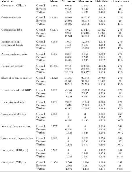
Table 8: Summary Statistics

Variable Mean Minimum Maximum Std. dev. Observations

Corruption (CPIt−1) Overall 2.665 0.000 7.010 1.822 273

Between 0.396 6.440 1.978 26

Within 1.669 4.729 0.438 10.5

Government size Overall 44.484 20.807 63.032 7.529 273

Between 24.894 56.978 7.135 26

Within 39.802 53.343 1.925 10.5

Government debt Overall 65.414 5.623 175.274 32.352 273